1 Introduction
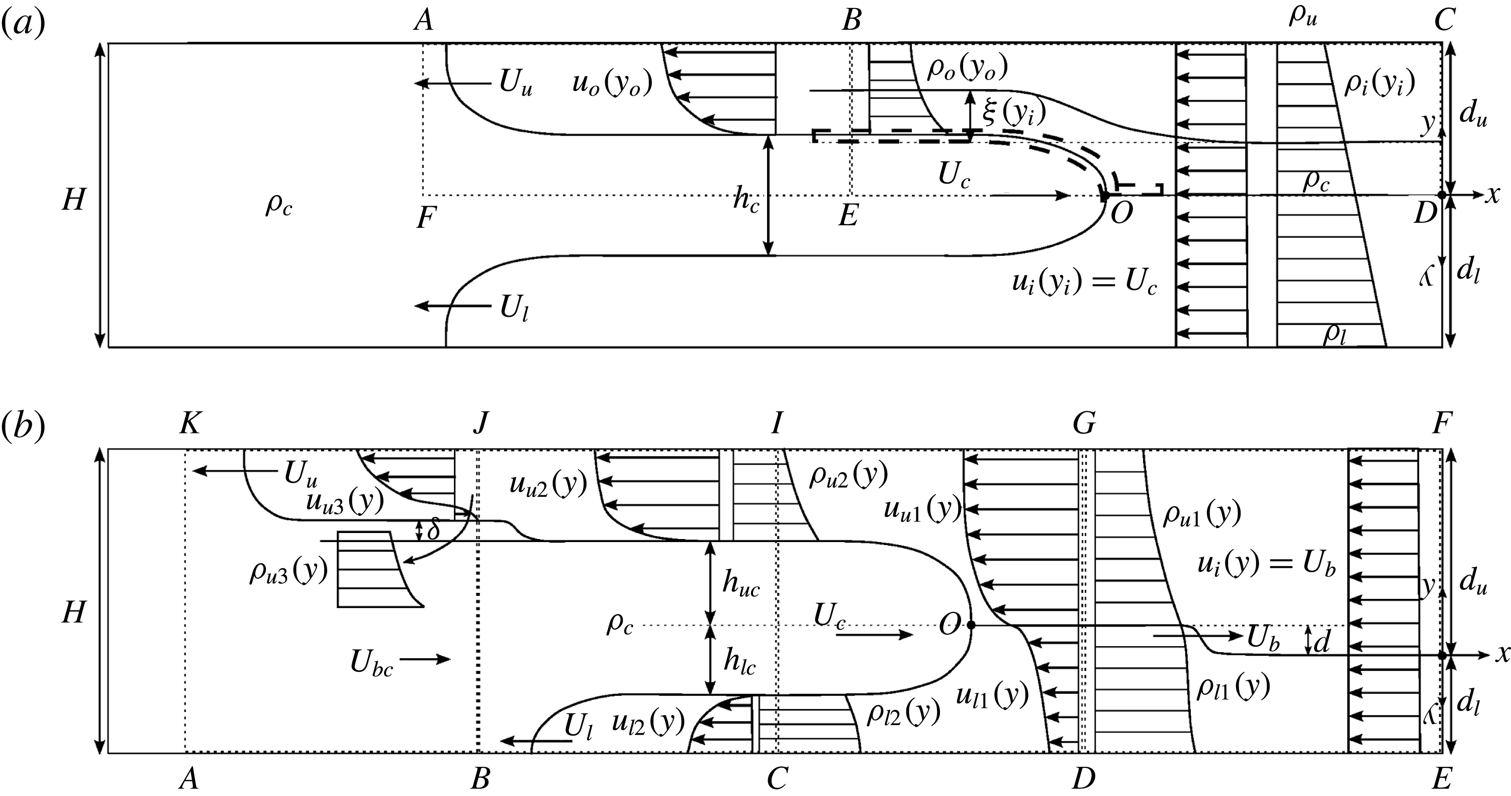
An intrusive gravity current, or intrusion, forms when a fluid of one density propagates laterally into a stratified ambient along an intermediate height. While several earlier studies addressed the case of two-layer stratified ambients (e.g. Holyer & Huppert Reference Holyer and Huppert1980; de Rooij, Linden & Dalziel Reference de Rooij, Linden and Dalziel1999; Lowe, Linden & Rottman Reference Lowe, Linden and Rottman2002; Sutherland, Kyba & Flynn Reference Sutherland, Kyba and Flynn2004; Cheong, Kuenen & Linden Reference Cheong, Kuenen and Linden2006; Flynn & Linden Reference Flynn and Linden2006; Khodkar, Nasr-Azadani & Meiburg Reference Khodkar, Nasr-Azadani and Meiburg2016), the current investigation focuses on intrusions propagating into linearly stratified ambients. Such flows can be generated in the laboratory via a lock-release experiment, as sketched in figure 1. The left half of a rectangular tank of length
 $L$
and height
 $H$
is initially filled with fluid of intermediate density
 $\unicode[STIX]{x1D70C}_{c}$
, while the right half contains a stratified fluid whose density varies linearly from
 $\unicode[STIX]{x1D70C}_{u}$
at the top to
 $\unicode[STIX]{x1D70C}_{l}$
at the bottom. Upon releasing the flow, the fluid of density
 $\unicode[STIX]{x1D70C}_{c}$
forms a right-propagating intrusion that travels with velocity
 $U_{c}$
. Concurrently, the ambient fluid forms two counterflowing gravity currents along the lower and upper walls that propagate with
 $U_{l}$
and
 $U_{u}$
, respectively. Earlier studies (Bolster, Hang & Linden Reference Bolster, Hang and Linden2008; Munroe et al.
Reference Munroe, Voegeli, Birman, Sutherland and Meiburg2009; Maurer, Bolster & Linden Reference Maurer, Bolster and Linden2010) demonstrate that the flow is symmetric with respect to the midplane of the tank when
 $\unicode[STIX]{x1D70C}_{c}=(\unicode[STIX]{x1D70C}_{l}+\unicode[STIX]{x1D70C}_{u})/2$
. Under these conditions, the neutral buoyancy isopycnal ahead of the intrusion remains flat, as shown in figure 1(a). On the other hand, when the intrusion density differs from the average ambient density, a non-symmetric intrusion forms as sketched in figure 1(b). Here the countercurrents along the top and bottom walls have different velocities, and the flow generates an upstream-propagating wave that travels ahead of the intrusion. Munroe et al. (Reference Munroe, Voegeli, Birman, Sutherland and Meiburg2009) and Maurer & Linden (Reference Maurer and Linden2014) observe that the wave amplitude varies across the tank height, and that this amplitude has a maximum near the neutral buoyancy isopycnal. A left-propagating bore also forms along the interface between the faster counterflowing current and the intrusion, at the streamwise location of the front of the slower counterflowing current. The degree of asymmetry in the flow can conveniently be expressed by the quantity
 $$\begin{eqnarray}\unicode[STIX]{x1D716}=\left|\frac{\unicode[STIX]{x1D70C}_{c}-0.5(\unicode[STIX]{x1D70C}_{u}+\unicode[STIX]{x1D70C}_{l})}{\unicode[STIX]{x1D70C}_{l}-\unicode[STIX]{x1D70C}_{u}}\right|.\end{eqnarray}$$
Lock-release flow of an intrusion into a linearly stratified ambient: (a) symmetric case; (b) non-symmetric case. For the symmetric case, the interface ahead of the intrusion remains unperturbed, whereas an upstream-propagating bore forms for the non-symmetric case. For the latter, the left-propagating gravity currents travel with different velocities, and the faster current gives rise to a bore at the same streamwise location as the front of the slower current. The dotted lines indicate the various control volumes for which mass and vorticity balances are established.

Efforts to develop analytical models for flows with arbitrary stratification date back over half a century. Based on the streamfunction–vorticity formulation for two-dimensional, incompressible, inviscid flows, Long (Reference Long1953) obtained a partial differential equation for the displacement of streamlines. Less general forms of this equation were later employed by Ungarish (Reference Ungarish2006) and White & Helfrich (Reference White and Helfrich2008) to study gravity currents travelling into linearly stratified ambients. The ordinary differential equation (ODE) derived by Nasr-Azadani & Meiburg (Reference Nasr-Azadani and Meiburg2016) for gravity currents advancing into linear stratification corresponds to the equation of Long (Reference Long1953), if derivatives are taken with respect to the upstream vertical coordinates of the streamlines.
The first analytical model for symmetric intrusions propagating into linearly stratified ambients was proposed by Ungarish (Reference Ungarish2005), based on a shallow-water approach. A similar model was also developed for bottom-propagating gravity currents in linear stratification by Ungarish & Huppert (Reference Ungarish and Huppert2002), while Ungarish & Huppert (Reference Ungarish and Huppert2006) compare the energy budget of the flow given by this one-layer shallow-water model with that provided by numerical simulations. This model considers intrusions during both the constant-velocity (slumping) and the time-dependent-velocity (self-similar) phases, and it investigates intrusions released from partial- as well as full-depth locks, cf. also Ungarish (Reference Ungarish2009).
Bolster et al. (Reference Bolster, Hang and Linden2008) develop a model for intrusions propagating into linearly stratified ambients by extending the approach of Cheong et al. (Reference Cheong, Kuenen and Linden2006). They obtain for the intrusion velocity
 $$\begin{eqnarray}\frac{U_{c}}{{\hat{g}}H}=\frac{F}{2}\sqrt{12\unicode[STIX]{x1D716}^{2}+1}.\end{eqnarray}$$
Depending on whether they calibrate with the results of Maxworthy et al. (Reference Maxworthy, Leilich, Simpson and Meiburg2002) or Ungarish (Reference Ungarish2006), they obtain
 $F$
-values of 0.266 or 0.25, respectively. Here
 ${\hat{g}}$
denotes the reduced gravity
 $g(\unicode[STIX]{x1D70C}_{l}-\unicode[STIX]{x1D70C}_{u})/\unicode[STIX]{x1D70C}_{c}$
. Bolster et al. (Reference Bolster, Hang and Linden2008) observe that the intrusion head becomes subcritical with respect to internal waves of mode-1 as soon as the symmetry condition is broken, and also with respect to internal waves of mode-2 as long as
 $\unicode[STIX]{x1D716}<0.23$
. They do not incorporate the wave energy into their model, based on the assumption that this energy component is much smaller than the potential and kinetic energies associated with the mean flow. An attempt to evaluate the contribution of the wave energy to the overall budget was made by Munroe et al. (Reference Munroe, Voegeli, Birman, Sutherland and Meiburg2009) and Maurer & Linden (Reference Maurer and Linden2014).
Within the current study, we extend the vorticity-based modelling concept to intrusive gravity currents propagating into linearly stratified ambients. This approach was first introduced by Borden & Meiburg (Reference Borden and Meiburg2013a ) and Borden & Meiburg (Reference Borden and Meiburg2013b ) for gravity currents and bores, and subsequently extended by Nasr-Azadani & Meiburg (Reference Nasr-Azadani and Meiburg2016) to flows with continuous stratification. It relies on the principles of mass and vorticity conservation only, and avoids the need for energy-related arguments. Based on the experimental observations of Munroe et al. (Reference Munroe, Voegeli, Birman, Sutherland and Meiburg2009), who showed that intrusions in linearly stratified ambients can propagate at constant speeds from 5 up to 20 times of the lock length (depending on whether the intrusion is symmetric or non-symmetric), we limit ourselves to the slumping phase and to the intrusions generated from a full-depth lock release. In addition, since we intend to focus on the upstream-propagating wave ahead of the intrusion, we take the lock length sufficiently long so that wave reflection from the rear wall will not be important. Section 2 develops vorticity models for both equilibrium and non-equilibrium intrusions. In § 3, we perform direct numerical simulations, whose results are compared in § 4 to the corresponding vorticity model predictions, as well as to theoretical and experimental findings of other authors. Section 5 presents a brief summary.
2 Theory
2.1 Symmetric intrusions
Due to their symmetry properties with respect to the channel centreline, symmetric intrusions can be analysed based on the upper half of the domain only, cf. figure 1(a). Hence, we are effectively dealing with a bottom gravity current propagating into a linearly stratified ambient in a domain of height
 $H/2$
. Nasr-Azadani & Meiburg (Reference Nasr-Azadani and Meiburg2016) analyse such flows under the assumption of inviscid vorticity dynamics in the Boussinesq limit, in the reference frame moving with the gravity current. We remark this assumption of inviscid vorticity dynamics does not necessarily imply that the flow is energy conserving. Nasr-Azadani & Meiburg (Reference Nasr-Azadani and Meiburg2016) show that the conservation of mass and vorticity result in a second-order ODE for the vertical displacement
 $\unicode[STIX]{x1D709}$
of a streamline between the upstream and downstream boundaries, as a function of its vertical inflow location
 $y_{i}$
 $$\begin{eqnarray}\unicode[STIX]{x1D709}^{\prime \prime }u_{i}^{2}+\unicode[STIX]{x1D709}^{\prime }(1+\unicode[STIX]{x1D709}^{\prime })(2+\unicode[STIX]{x1D709}^{\prime })u_{i}u_{i}^{\prime }-\unicode[STIX]{x1D709}(1+\unicode[STIX]{x1D709}^{\prime })^{3}g\frac{\unicode[STIX]{x1D70C}_{i}^{\prime }}{\unicode[STIX]{x1D70C}_{c}}=0.\end{eqnarray}$$
Here
 $\unicode[STIX]{x1D70C}_{i}(y_{i})$
and
 $u_{i}(y_{i})$
denote the density and horizontal velocity distributions at the inflow boundary, respectively.
 $y_{i}$
varies from 0 to
 $H/2$
, where
 $y_{i}=0$
is located at the neutral buoyancy isopycnal
 $y_{N}$
 $$\begin{eqnarray}y_{N}=\left(1-\frac{\unicode[STIX]{x1D70C}_{c}-\unicode[STIX]{x1D70C}_{u}}{\unicode[STIX]{x1D70C}_{l}-\unicode[STIX]{x1D70C}_{u}}\right)H,\end{eqnarray}$$
which is identical to the channel centreline for symmetric intrusions. Substituting the upstream flow conditions corresponding to figure 1(a) into (2.1) results in
 $$\begin{eqnarray}\unicode[STIX]{x1D709}^{\prime \prime }U_{c}^{2}+\unicode[STIX]{x1D709}(1+\unicode[STIX]{x1D709}^{\prime })^{3}gN^{2}=0,\end{eqnarray}$$
with buoyancy frequency
 $N$
equal to
 $\sqrt{g(\unicode[STIX]{x1D70C}_{l}-\unicode[STIX]{x1D70C}_{u})/(\unicode[STIX]{x1D70C}_{c}H)}$
. As boundary conditions we have
 $\unicode[STIX]{x1D709}(H/2)=0$
and
 $\unicode[STIX]{x1D709}(0)=h_{c}/2$
, where the intrusion height
 $h_{c}$
is unknown. Vorticity conservation along the upper interface of the intrusion gives
 $$\begin{eqnarray}\frac{u_{o}(0)^{2}}{2}=g\frac{\unicode[STIX]{x1D70C}_{i}(0)-\unicode[STIX]{x1D70C}_{c}}{\unicode[STIX]{x1D70C}_{c}}\frac{h_{c}}{2}=0,\end{eqnarray}$$
where
 $u_{o}$
indicates the horizontal velocity at the outflow boundary of control volume
 $EDCB$
. This equation is obtained by applying the vorticity conservation principle to the infinitesimal control volume whose top and bottom boundaries are immediately above and below the upper interface of the intrusion (dashed lines in figure 1
a). Clearly there is no influx of vorticity into this control volume, since the upstream velocity is uniform. Furthermore, as the width of this control volume decreases, the density difference across the outflow boundary of the control volume decreases as well, and it tends to zero in the limit of a vanishingly thin control volume, so that no vortex sheet forms along the interface. Hence, at the interface the ambient has the same velocity as the intrusion, so that
 $u_{o}(0)=0$
in the reference frame moving with the intrusion. By applying the conservation of mass to an infinitesimal streamtube, Nasr-Azadani & Meiburg (Reference Nasr-Azadani and Meiburg2016) show
 $$\begin{eqnarray}u_{o}(y_{i})=\frac{u_{i}(y_{i})}{1+\unicode[STIX]{x1D709}^{\prime }},\end{eqnarray}$$
so that we obtain
 $\unicode[STIX]{x1D709}^{\prime }(0)=\infty$
. This boundary condition is different from those of Ungarish (Reference Ungarish2006) and White & Helfrich (Reference White and Helfrich2008) for boundary-propagating gravity currents, since both of those studies obtain their closure equation from using Bernoulli’s equation. An additional equation for the unknown intrusion thickness
 $h_{c}$
can be obtained by applying the inviscid integral vorticity conservation equation
 $$\begin{eqnarray}\oint \unicode[STIX]{x1D714}\boldsymbol{u}\boldsymbol{\cdot }\boldsymbol{n}\,\text{d}S=-\iint \frac{g}{\unicode[STIX]{x1D70C}_{c}}\frac{\unicode[STIX]{x2202}\unicode[STIX]{x1D70C}}{\unicode[STIX]{x2202}x}\,\text{d}A,\end{eqnarray}$$
to control volume
 $FEBA$
in the reference frame moving leftward with the velocity
 $U_{u}$
of the upper gravity current. Here
 $\unicode[STIX]{x1D714}$
and
 $\boldsymbol{u}$
represent the vorticity normal to the plane and the velocity vector, respectively.
 $\text{d}A$
,
 $\text{d}S$
and
 $\boldsymbol{n}$
indicate a differential area within the control volume, a differential length along the boundaries of the control volume and the unit outer normal vector to the control volume boundaries. For
 $FEBA$
, equation (2.6) reduces to
 $$\begin{eqnarray}\frac{1}{2}\Big\{(U_{u}+U_{c})^{2}-\big[U_{u}-\big(u_{o}(H/2)-U_{c}\big)\big]^{2}\Big\}=\int _{h_{c}/2}^{H/2}\frac{g}{\unicode[STIX]{x1D70C}_{c}}\big[\unicode[STIX]{x1D70C}_{c}-\unicode[STIX]{x1D70C}_{o}(y)\big]\,\text{d}y.\end{eqnarray}$$
We evaluate
 $U_{u}$
as the average horizontal velocity within the upper gravity current in the laboratory frame
 $$\begin{eqnarray}U_{u}=\frac{\displaystyle \int _{h_{c}/2}^{H/2}\big[u_{o}(y)-U_{c}\big]\,\text{d}y}{H/2-h_{c}/2}.\end{eqnarray}$$
Here
 $U_{u}-[u_{o}(H/2)-U_{c}]$
is the horizontal velocity along the top wall at
 $B$
, in the reference frame moving with the upper gravity current.
We can then solve the vorticity model equations as follows: after guessing initial values for
 $h_{c}$
and
 $U_{c}$
, we integrate equation (2.3) subject to the boundary conditions
 $\unicode[STIX]{x1D709}(0)=h_{c}/2$
and
 $\unicode[STIX]{x1D709}^{\prime }(0)=\infty$
. The latter is implemented by setting
 $\unicode[STIX]{x1D709}^{\prime }(0)$
to a large number. Tests show that for sufficiently large values
 $\unicode[STIX]{x1D709}^{\prime }(0)>10^{3}$
, the numerical solution does not depend on the exact value chosen. Then we perform an inner iteration loop by updating our guess for
 $h_{c}$
via a bisection shooting procedure until the condition
 $|\unicode[STIX]{x1D709}(H/2)|<10^{-7}$
is satisfied. The final value for
 $U_{c}$
is then found via an outer iteration loop, as follows: since the density remains constant along a streamline, we can evaluate the outflow density
 $\unicode[STIX]{x1D70C}_{o}(y)$
from
 $\unicode[STIX]{x1D70C}_{o}(y_{i}+\unicode[STIX]{x1D709}(y_{i}))=\unicode[STIX]{x1D70C}_{i}(y_{i})$
, and the outflow velocity
 $u_{o}(y)$
is obtained from (2.5). We then iterate on
 $U_{c}$
until (2.7) is satisfied within the control volume
 $FEBA$
with an error less than
 $10^{-7}$
.
2.2 Non-symmetric intrusions
If the symmetry condition is violated, a non-equilibrium intrusion such as the one sketched in figure 1(b) forms, giving rise to an upstream-propagating wave. This wave travels with uniform velocity for all isopycnals (Munroe et al.
Reference Munroe, Voegeli, Birman, Sutherland and Meiburg2009; Maurer & Linden Reference Maurer and Linden2014)). Its amplitude vanishes at the top and bottom walls and has a maximum close to the neutral buoyancy isopycnal, as discussed earlier. In the following, we treat this leading wave as a bore that has an amplitude
 $d$
at the neutral buoyancy isopycnal and travels with velocity
 $U_{b}$
. The validity of this assumption will be further examined in § 4. To solve for the speed and the amplitude of this bore, we employ a vorticity-based analysis similar to that of § 2.1, by applying (2.1) separately to the upper and lower regions of control volume
 $DEFG$
, in the reference frame moving with the bore. We thus obtain
 $$\begin{eqnarray}\unicode[STIX]{x1D709}^{\prime \prime }U_{b}^{2}+\unicode[STIX]{x1D709}(1+\unicode[STIX]{x1D709}^{\prime })^{3}N^{2}=0.\end{eqnarray}$$
The
 $y$
-axis is directed upward in the upper region, and downward in the lower region, so that the form of (2.9) remains identical in both regions. As boundary conditions at the interface and the upper and lower walls we have
 $$\begin{eqnarray}\displaystyle & \unicode[STIX]{x1D709}_{u1}(0)=-\unicode[STIX]{x1D709}_{l1}(0)=d, & \displaystyle\end{eqnarray}$$
 $$\begin{eqnarray}\displaystyle & \unicode[STIX]{x1D709}_{u1}(d_{u})=\unicode[STIX]{x1D709}_{l1}(d_{l})=0. & \displaystyle\end{eqnarray}$$
Furthermore, the solution has to be smooth at the interface, so that
 $$\begin{eqnarray}\unicode[STIX]{x1D709}_{u1}^{\prime }(0)=\unicode[STIX]{x1D709}_{l1}^{\prime }(0).\end{eqnarray}$$
We then set up an iterative solution procedure, with an inner loop for
 $U_{b}$
and an outer one for
 $d$
, along the following lines: based on initial guesses for these two variables we solve (2.9) for the upper and lower regions based on boundary conditions (2.10) and (2.11), via a bisection shooting method. In this way we obtain the slopes of the deflection at the neutral buoyancy isopycnal
 $\unicode[STIX]{x1D709}_{u1}^{\prime }(0)$
and
 $\unicode[STIX]{x1D709}_{l1}^{\prime }(0)$
. We then iterate on
 $U_{b}$
until (2.12) holds. We verify the validity of the
 $d$
-value later, and iterate on that, if needed.
The above provides us with preliminary density and velocity distributions upstream of the intrusion. Due to the propagation of internal gravity waves upstream of the intrusion, the density stratification ahead of the intrusion will no longer be linear and the velocity distribution exhibits shear, so that the more general equation (2.1) has to be employed to obtain the intrusion speed and thickness. Towards this end, we first investigate the flow within the slower left-propagating current, which is the lower one when
 $\unicode[STIX]{x1D70C}_{c}>(\unicode[STIX]{x1D70C}_{l}+\unicode[STIX]{x1D70C}_{u})/2$
. Next, we guess a value for
 $U_{c}$
and shift the reference frame from the leading bore to the intrusion by replacing
 $u_{i}$
with
 $u_{l1}-U_{b}+U_{c}$
in (2.1). We then find the thicknesses of the lower gravity current and lower branch of the intrusion,
 $h_{l}$
and
 $h_{lc}$
, as well as the intrusion speed
 $U_{c}$
by using the same numerical procedure as that described for a symmetric intrusion, except that the closure equation should be modified as we apply the vorticity conservation equation (2.6) to the region below the stagnation point of the intrusion (
 $O$
in figure 1
b) and inside control volume
 $BCIJ$
, while travelling with the bottom-propagating current, which leads to
 $$\begin{eqnarray}\frac{1}{2}\Big\{(U_{l}+U_{c})^{2}-\big[U_{l}-(u_{l2}(d_{l}+d)-U_{c})\big]^{2}\Big\}=\int _{h_{lc}}^{d_{l}+d}\frac{g}{\unicode[STIX]{x1D70C}_{c}}(\unicode[STIX]{x1D70C}_{l2}(y)-\unicode[STIX]{x1D70C}_{c})\,\text{d}y.\end{eqnarray}$$
 $U_{l}$
in the above equation can be calculated in the same fashion as
 $U_{u}$
in § 2.1
 $$\begin{eqnarray}U_{l}=\frac{\displaystyle \int _{h_{lc}}^{d_{l}+d}\big[u_{l2}(y)-U_{c}\big]\,\text{d}y}{h_{l}}.\end{eqnarray}$$
Computing
 $U_{c}$
enables us to solve for the flow properties within the upper branch of the intrusion, when we substitute
 $u_{i}$
and
 $\unicode[STIX]{x1D70C}_{i}$
with
 $u_{u1}-U_{b}+U_{c}$
and
 $\unicode[STIX]{x1D70C}_{u1}$
. We then guess a value for
 $h_{uc}$
and correct our guess until integrating from ODE (2.1) yields
 $|\unicode[STIX]{x1D709}_{u2}(d_{u}-d)|<10^{-7}$
. The thickness
 $h_{c}$
of the intrusion can then be computed as
 $h_{lc}+h_{uc}$
.
Evaluation of the flow variables downstream of the intrusion then allows us to determine the properties of the left-propagating internal bore, which travels at the same speed as the slower counterflowing current (here
 $U_{l}$
). Thus, we only need to find its amplitude to obtain the flow condition downstream of the bore. Towards this end, we make a guess for the amplitude
 $\unicode[STIX]{x1D6FF}$
and solve (2.1) in an iterative fashion, with slope
 $\unicode[STIX]{x1D709}_{u3}^{\prime }(0)$
equal to
 $$\begin{eqnarray}\unicode[STIX]{x1D709}_{u3}^{\prime }(0)=\frac{U_{c}+U_{l}}{U_{bc}+U_{l}}-1.\end{eqnarray}$$
This condition is obtained using (2.5) along the interface of the bore.
 $U_{bc}$
can also be calculated by employing the continuity equation within the intrusion fluid and in the reference frame moving with the left-propagating bore
 $$\begin{eqnarray}(U_{bc}+U_{l})(H-h_{u})=(U_{c}+U_{l})h_{c}.\end{eqnarray}$$
This ODE has to be solved concurrently along with (2.15) and (2.16) to obtain the bore amplitude
 $\unicode[STIX]{x1D6FF}$
in addition to the flow properties downstream of the bore.
The above analysis evaluates the properties of all flow components for the preliminary
 $d$
-value. The validity of this
 $d$
-value can then be checked by examining the vorticity balance within the entire control volume
 $ABJK$
, in the reference frame moving with the top-propagating current. This yields
 $$\begin{eqnarray}\frac{1}{2}\Big\{(U_{u}+U_{bc})^{2}-\big[U_{u}-(u_{u3}(H)+U_{l})\big]^{2}\Big\}=\int _{H-h_{u}}^{H}\frac{g}{\unicode[STIX]{x1D70C}_{c}}\big[\unicode[STIX]{x1D70C}_{c}-\unicode[STIX]{x1D70C}_{u3}(y)\big]\,\text{d}y,\end{eqnarray}$$
where
 $h_{u}=H-h_{c}-h_{l}-\unicode[STIX]{x1D6FF}$
. If (2.17) holds to within
 $10^{-7}$
, we accept the preliminary
 $d$
-value, otherwise we iterate to obtain an updated value for
 $d$
.
3 Direct numerical simulation results
To assess the predictive capabilities of the vorticity model, we perform two-dimensional direct numerical simulations with our in-house software TURBINS (Nasr-Azadani & Meiburg Reference Nasr-Azadani and Meiburg2011; Nasr-Azadani, Hall & Meiburg Reference Nasr-Azadani, Hall and Meiburg2013). Based on a finite-difference approach that utilizes a fractional projection method along with total variation diminishing third-order Runge–Kutta (TVD-RK3) time integration, TURBINS solves the dimensionless Navier–Stokes and density equations in the Boussinesq limit
 $$\begin{eqnarray}\displaystyle & \displaystyle \unicode[STIX]{x1D735}\boldsymbol{\cdot }\boldsymbol{u}^{\ast }=0, & \displaystyle\end{eqnarray}$$
 $$\begin{eqnarray}\displaystyle & \displaystyle \frac{\unicode[STIX]{x2202}\boldsymbol{u}^{\ast }}{\unicode[STIX]{x2202}t^{\ast }}+\boldsymbol{u}^{\ast }\boldsymbol{\cdot }\unicode[STIX]{x1D735}\boldsymbol{u}^{\ast }=-\unicode[STIX]{x1D735}p^{\ast }+\frac{1}{Re}\unicode[STIX]{x1D6FB}^{2}\boldsymbol{u}^{\ast }+\unicode[STIX]{x1D70C}^{\ast }\boldsymbol{e}^{g}, & \displaystyle\end{eqnarray}$$
 $$\begin{eqnarray}\displaystyle & \displaystyle \frac{\unicode[STIX]{x2202}\unicode[STIX]{x1D70C}^{\ast }}{\unicode[STIX]{x2202}t^{\ast }}+\boldsymbol{u}^{\ast }\boldsymbol{\cdot }\unicode[STIX]{x1D735}\unicode[STIX]{x1D70C}^{\ast }=\frac{1}{Pe}\unicode[STIX]{x1D6FB}^{2}\unicode[STIX]{x1D70C}^{\ast }. & \displaystyle\end{eqnarray}$$
Here,
 $\boldsymbol{e}^{g}$
denotes the unit vector in the direction of gravity. The Reynolds and Péclet numbers are defined as
 $Re=\sqrt{{\hat{g}}H}H/\unicode[STIX]{x1D708}$
and
 $Pe=\sqrt{{\hat{g}}H}H/D$
, where
 $H$
,
 $\unicode[STIX]{x1D708}$
and
 $D$
represent the channel height, kinematic viscosity and diffusivity of the density field. For the purpose of non-dimensionalization, the reference length, velocity and pressure are taken as
 $H$
,
 $\sqrt{{\hat{g}}H}$
and
 $\unicode[STIX]{x1D70C}_{c}{\hat{g}}H$
, respectively. The dimensionless density is defined as
 $\unicode[STIX]{x1D70C}^{\ast }=(\unicode[STIX]{x1D70C}-\unicode[STIX]{x1D70C}_{u})/(\unicode[STIX]{x1D70C}_{l}-\unicode[STIX]{x1D70C}_{u})$
.
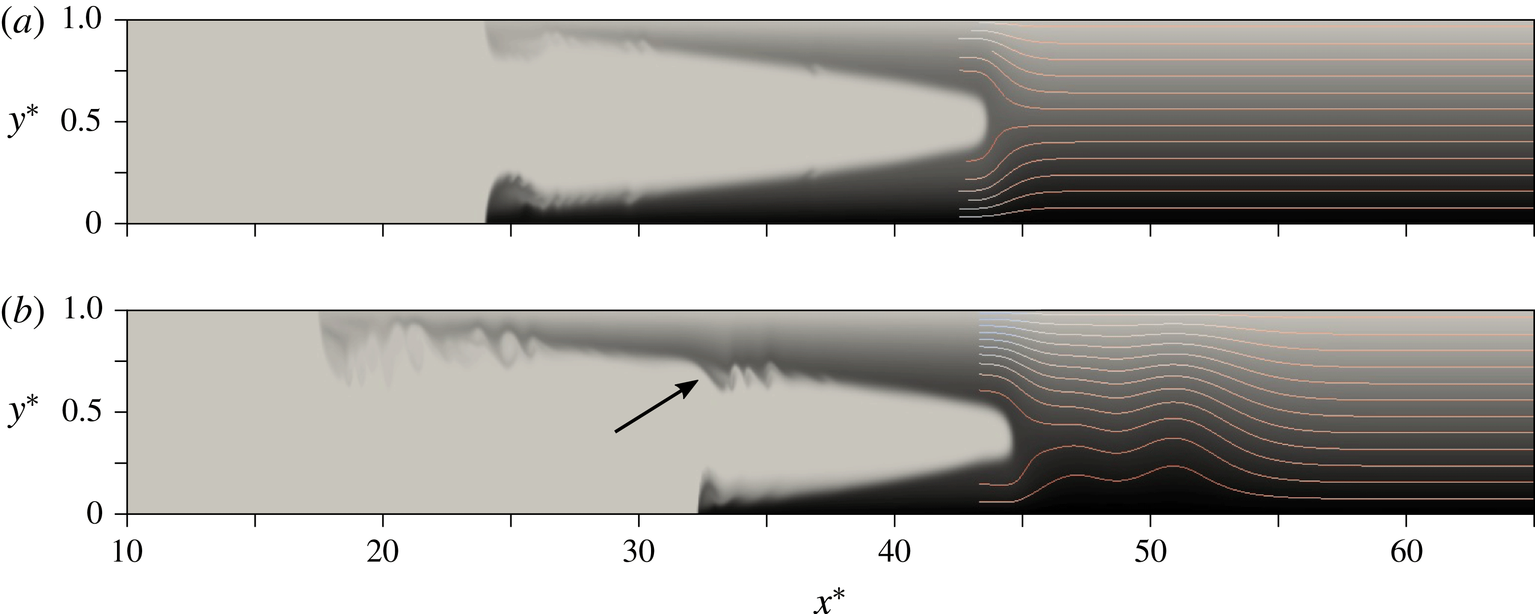
Density fields at time
 $t^{\ast }=60$
for (a) a symmetric intrusion, and (b) a non-symmetric intrusion with
 $\unicode[STIX]{x1D70C}_{c}^{\ast }=0.7$
. The arrow in panel (b) indicates the location of the left-propagating bore. Streamlines upstream of the intrusion are shown in the reference frame moving with the intrusion. Inside the ambient, the density field varies from
 $\unicode[STIX]{x1D70C}^{\ast }=0$
(light grey) to
 $\unicode[STIX]{x1D70C}^{\ast }=1$
(black). The intrusion fluid is shown in light grey, in order to help distinguish it from the ambient fluid.

We employ free-slip conditions at all boundaries, along with vanishing normal flux conditions for the density field. Initially, the fluid is at rest everywhere. The left half of the container is filled with the intrusion fluid of constant density
 $\unicode[STIX]{x1D70C}_{c}^{\ast }$
, while the stratified ambient fluid in the right half of the container has an initial density profile
 $\unicode[STIX]{x1D70C}^{\ast }=1-y^{\ast }$
. The simulations are carried out for
 $Re=3\times 10^{4}$
and
 $Pe=7.5\times 10^{4}$
, so that diffusive effects can be assumed small. The computational domain has dimensions
 $L=70$
and
 $H=1$
, and we employ a uniformly spaced grid with
 $\unicode[STIX]{x0394}x^{\ast }=0.01$
and
 $\unicode[STIX]{x0394}y^{\ast }=0.005$
.
For a representative symmetric intrusion, figure 2(a) shows the density field at
 $t^{\ast }=60$
, along with streamlines in the reference frame moving with the intrusion. The neutral buoyancy isopycnal remains undisturbed ahead of the intrusion front, consistent with the assumption of the model developed in § 2.1 for symmetric intrusions (
 $\unicode[STIX]{x1D70C}_{c}^{\ast }=0.5$
). On the other hand, the non-symmetric counterpart in figure 2(b) clearly indicates the presence of a wavefront that propagates faster than the intrusion itself. By conducting simulations for different values of
 $\unicode[STIX]{x1D716}$
, we found that for
 $\unicode[STIX]{x1D716}\lesssim 0.2$
the flow typically gives rise to both mode-1 and mode-2 internal waves, with the mode-1 waves travelling nearly twice as fast as the mode-2 waves. For
 $\unicode[STIX]{x1D716}\gtrsim 0.2$
, the simulations showed mode-1 waves only. This observation is consistent with earlier findings by Munroe et al. (Reference Munroe, Voegeli, Birman, Sutherland and Meiburg2009) and Maurer & Linden (Reference Maurer and Linden2014). We remark that these waves are more directly comparable to those observed by Maurer & Linden (Reference Maurer and Linden2014), rather than to the waves reflected from the rear wall identified by Munroe et al. (Reference Munroe, Voegeli, Birman, Sutherland and Meiburg2009). In contrast to earlier studies, we note that the waviness of the isopycnals in figure 2(b) exhibits two distinguishable peaks, which can be attributed to the longer locks employed here. In addition, the simulations showed that the deflections of all isopycnals travel at the same speed, and that the maximum deflection always occurs close to the neutral buoyancy isopycnal, which allows us to treat the leading wave as a hydraulic bore.
In order to track the intrusion and ambient fluids, we mark them with different passive ‘computational dyes’ that have the same diffusivity as the density field. If we denote the dimensionless dye concentration by
 $c_{d}^{\ast }$
, we can define the local height
 $\unicode[STIX]{x1D702}^{\ast }$
of the right-propagating intrusions or the left-propagating gravity currents as
 $$\begin{eqnarray}\displaystyle \unicode[STIX]{x1D702}^{\ast }(x^{\ast },t^{\ast })=\int _{0}^{1}c_{d}^{\ast }(x^{\ast },y^{\ast },t^{\ast })\,\text{d}y^{\ast }. & & \displaystyle\end{eqnarray}$$
The front location
 $x_{f}^{\ast }$
of a current is then obtained as the first point with
 $\unicode[STIX]{x1D702}^{\ast }>0.01$
.
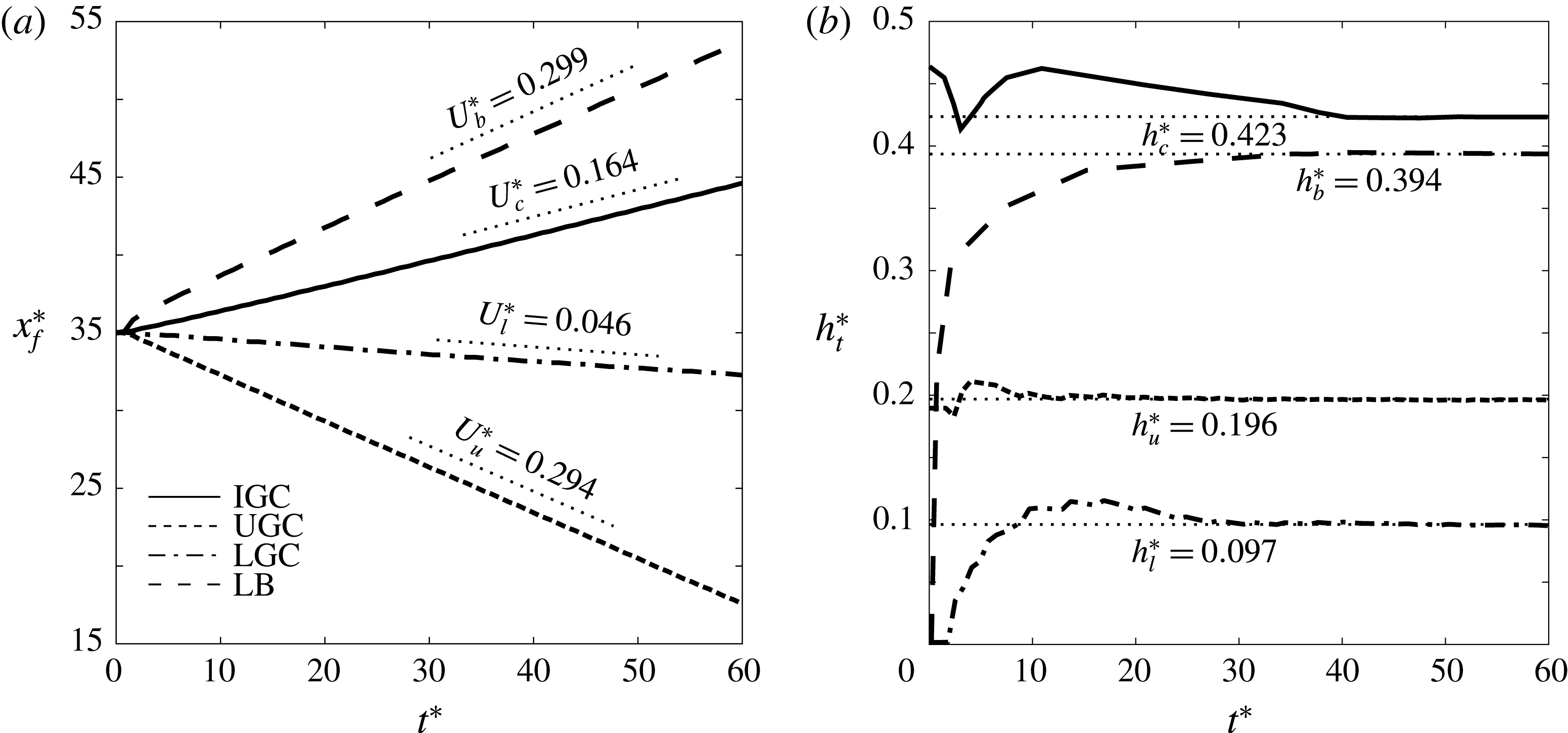
(a) Front locations, and (b) current thicknesses as functions of time, for the direct numerical simulation (DNS) of figure 2(b). IGC, UGC and LGC denote the intrusive, upper and lower gravity currents, respectively, while LB refers to the leading bore. The straight line segments in panel (a) represent the quasisteady front velocities, obtained by linear fits of the DNS results, while the dotted lines in panel (b) indicate the quasisteady heights, evaluated as described in the text.

Figure 3(a) depicts the front locations of the upper and lower gravity currents and the intrusion as functions of time, for the non-symmetric intrusion of figure 2(b). After a brief transient period all three fronts are seen to acquire quasisteady velocities, as indicated by the dotted straight line segments. We can then define an effective, time-dependent intrusion height
 $h_{t,c}^{\ast }$
by averaging the local intrusion height from the gate location to the intrusion front. The heights
 $h_{t,l}^{\ast }$
and
 $h_{t,u}^{\ast }$
of the lower and upper gravity currents are calculated correspondingly. Figure 3(b) indicates that all current heights approach quasisteady values beyond
 $t^{\ast }=40$
, so that we can obtain time-independent current heights
 $h^{\ast }$
by averaging the DNS results from
 $t^{\ast }=40$
to
 $t^{\ast }=60$
.
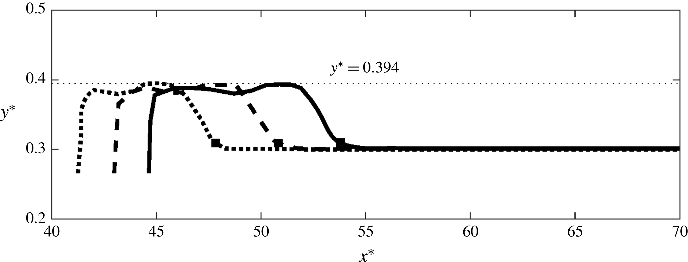
Temporal evolution of the neutral buoyancy isopycnal regarding the flow shown in figure 2(b), for times
 $t^{\ast }=40$
(dotted line), 50 (dashed line) and 60 (solid line). The black squares represent the respective front locations of the bore at these times. The horizontal dotted line indicates the quasisteady value of the maximum height
 $h_{b}^{\ast }$
of the neutral buoyancy isopycnal.

Figure 4 represents the shape of the neutral buoyancy isopycnal for the simulation of figure 2(b), for three different times in the quasisteady regime. The figure confirms that the front of this isopycnal propagates in a bore-like fashion. We define the front location
 $x_{f,b}^{\ast }$
of this bore, indicated by black squares, as the rightmost point along the neutral buoyancy isopycnal where its vertical coordinate is 0.01 above the neutral buoyancy level
 $y_{N}^{\ast }$
. An effective height
 $h_{b}^{\ast }$
of the neutral buoyancy isopycnal downstream of the bore is obtained by temporally averaging the instantaneous maximum height
 $h_{t,b}^{\ast }$
of this isopycnal between
 $t^{\ast }=40$
and
 $t^{\ast }=60$
, as indicated by the horizontal dotted line in figure 4. The bore amplitude
 $d^{\ast }$
is then calculated as
 $d^{\ast }=|h_{b}^{\ast }-y_{N}^{\ast }|$
.
For the non-symmetric intrusion of figure 2(b), the bore location
 $x_{f,b}^{\ast }$
and its instantaneous maximum height
 $h_{t,b}^{\ast }$
are shown in figure 3 as functions of time. We recognize that for large times both the bore velocity and the bore height achieve quasisteady values. By carrying out a corresponding analysis for other isopycnals, we confirm that all of them propagate with the same velocity. This procedure furthermore yields the displacement magnitude as function of the isopycnal. We find that the largest displacement value
 $d_{max}^{\ast }$
occurs close to the neutral buoyancy level. We refer to
 $d_{max}^{\ast }$
as the maximum wave amplitude, consistent with Munroe et al. (Reference Munroe, Voegeli, Birman, Sutherland and Meiburg2009) and Maurer & Linden (Reference Maurer and Linden2014).
4 Comparison of model predictions and simulation results
Figure 5 displays the propagation velocity
 $U_{b}^{\ast }$
and the amplitude
 $d^{\ast }$
of the bore, along with the maximum deflection
 $d_{max}^{\ast }$
of the isopycnals, as functions of
 $\unicode[STIX]{x1D70C}_{c}^{\ast }$
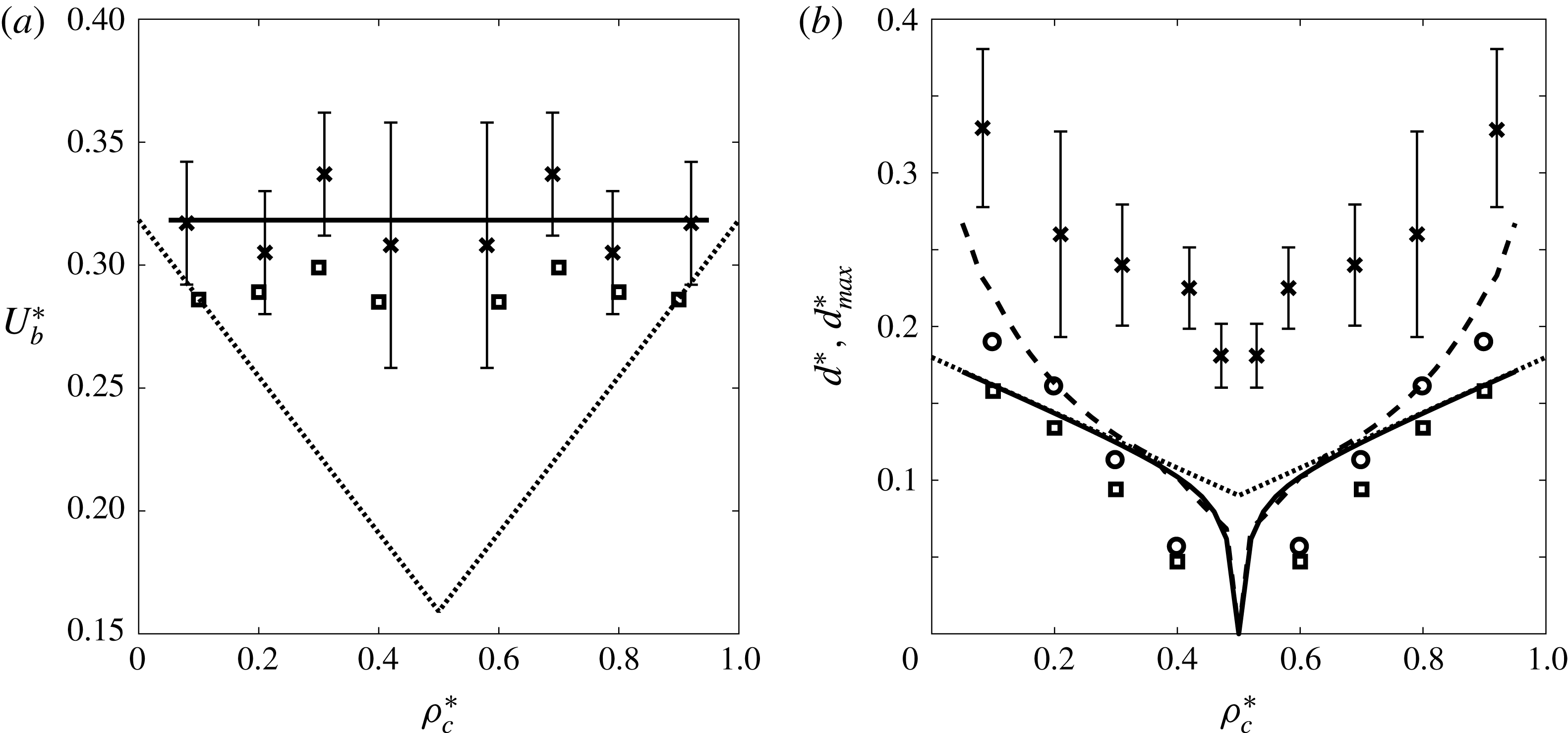
. Shown are DNS results, vorticity model predictions, the estimates of Munroe et al. (Reference Munroe, Voegeli, Birman, Sutherland and Meiburg2009) and the experimental data reported by Maurer & Linden (Reference Maurer and Linden2014). The vorticity model predicts a constant bore propagation velocity
 $U_{b}^{\ast }\approx 1/\unicode[STIX]{x03C0}$
, which is the theoretical propagation velocity of linear mode-1 waves (McEwan & Baines Reference McEwan and Baines1974). Since non-symmetric intrusions always give rise to mode-1 waves, and since these travel faster than any higher-order modes, it is consistent that the leading wave front travels with this velocity. The fact that mode-2 waves are symmetric with respect to the midplane of the tank, so that they result in smaller net displacements of the isopycnals (Bolster et al.
Reference Bolster, Hang and Linden2008), further supports this observation. By itself, the vorticity model does not yield any information with regard to the propagation velocity and amplitude of the mode-2 waves. In order to obtain such information, one would have to employ the full ODE to account for the waviness of the isopycnals upstream of the intrusion. The vorticity model predictions regarding
 $U_{b}^{\ast }$
generally agree with the DNS results to within about 10 %. They are also in reasonable agreement with experimental results of Maurer & Linden (Reference Maurer and Linden2014). Especially for near-symmetric intrusions, this is somewhat closer than the empirical formula of Munroe et al. (Reference Munroe, Voegeli, Birman, Sutherland and Meiburg2009). For
 $\unicode[STIX]{x1D716}\rightarrow 0.5$
(or
 $\unicode[STIX]{x1D70C}_{c}^{\ast }\rightarrow 0,1$
), on the other hand, the vorticity model predictions agree closely with this empirical formula. As shown in figure 5(b) the vorticity model predicts that
 $d^{\ast }\approx d_{max}^{\ast }$
for near-equilibrium intrusions, while they increasingly differ from each other as
 $\unicode[STIX]{x1D716}$
grows. Interestingly, for strongly non-symmetric intrusions the vorticity model predictions for
 $d^{\ast }$
are very close to the
 $d_{max}^{\ast }$
-estimates of Munroe et al. (Reference Munroe, Voegeli, Birman, Sutherland and Meiburg2009). The vorticity model predictions for both
 $d^{\ast }$
and
 $d_{max}^{\ast }$
generally agree well with corresponding DNS results, although there is a noticeable discrepancy in regard to the experimental data of Maurer & Linden (Reference Maurer and Linden2014).
(a) Propagation speed
 $U_{b}^{\ast }$
of the bore, and (b) maximum displacement
 $d^{\ast }$
of the neutral buoyancy isopycnal as well as the maximum isopycnal deflection
 $d_{max}^{\ast }$
, as functions of the dimensionless intrusion density
 $\unicode[STIX]{x1D70C}_{c}^{\ast }$
. In panel (a), the solid line represents the vorticity model prediction, while the dotted line indicates the estimate of Munroe et al. (Reference Munroe, Voegeli, Birman, Sutherland and Meiburg2009). The discrete squares and crosses also denote the DNS results and experimental results of Maurer & Linden (Reference Maurer and Linden2014). In panel (b), the solid and dashed lines represent the vorticity model predictions for
 $d^{\ast }$
and
 $d_{max}^{\ast }$
, respectively, while the dotted line indicates the estimate of Munroe et al. (Reference Munroe, Voegeli, Birman, Sutherland and Meiburg2009) for
 $d_{max}^{\ast }$
. The discrete squares, circles and crosses reflect the DNS results for
 $d^{\ast }$
and
 $d_{max}^{\ast }$
as well as the experimental data reported by Maurer & Linden (Reference Maurer and Linden2014) for
 $d_{max}^{\ast }$
, respectively.

Dependence of various flow properties on the dimensionless intrusion density
 $\unicode[STIX]{x1D70C}_{c}^{\ast }$
: (a) intrusion front velocity
 $U_{c}^{\ast }$
, (b) intrusion thickness
 $h_{c}^{\ast }$
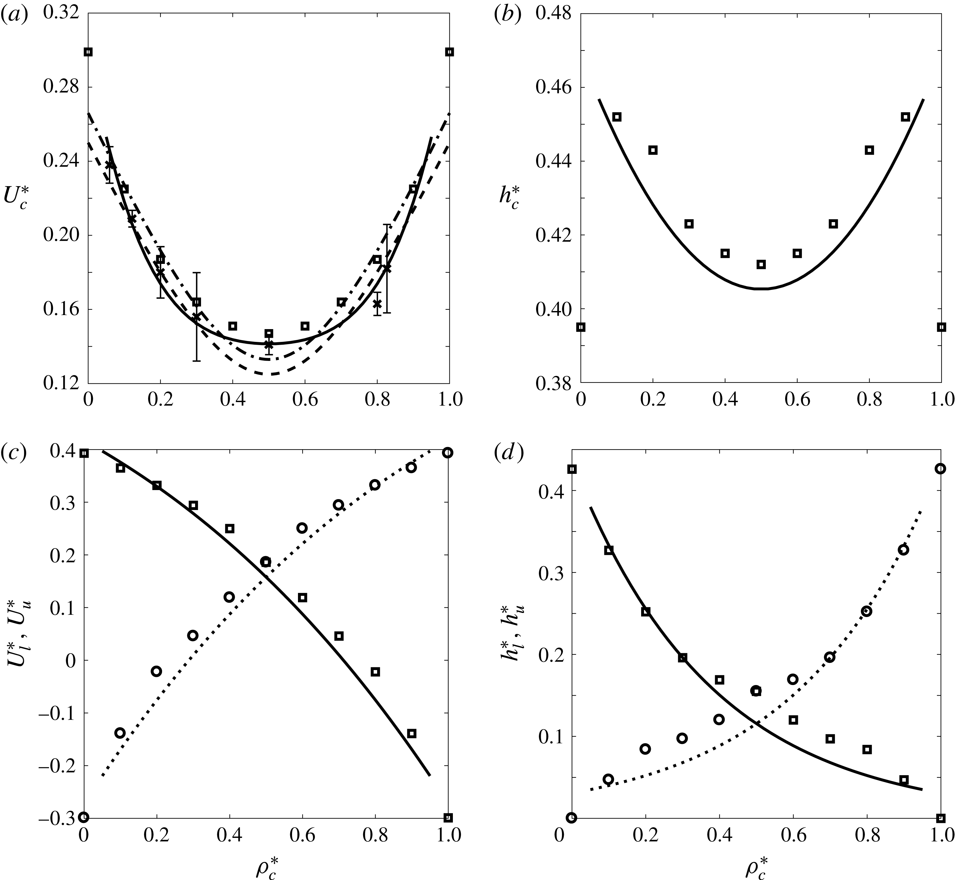
, (c) front velocities of the left-propagating gravity currents and (d) thicknesses of the left-propagating gravity currents. The solid lines represent the vorticity model predictions for the intrusion and lower gravity current properties, while the dotted lines denote the corresponding predictions for the upper gravity current. The dashed and dash-dotted lines indicate the results of Bolster et al. (Reference Bolster, Hang and Linden2008) for the intrusion speed, when
 $F=0.25$
and 0.266, respectively. The discrete circles and squares reflect the present DNS results, while the discrete crosses represent the experimental data of Bolster et al. (Reference Bolster, Hang and Linden2008).

Figure 6 shows model predictions, experimental data and DNS results for the propagation velocities and thicknesses of all three fronts, as functions of
 $\unicode[STIX]{x1D70C}_{c}^{\ast }$
. Figure 6(a) demonstrates good agreement among all data sets regarding the intrusion velocity.
 $U_{c}^{\ast }$
for equilibrium intrusions can furthermore be compared to the result of Ungarish (Reference Ungarish2005) for an intrusion propagating in a linearly stratified tank, and to the finding of Ungarish (Reference Ungarish2006) for a bottom-propagating gravity current whose density is identical to that at the base of the stratification. Both of these results are slightly larger than, but within 5 % of the vorticity model prediction. The small difference between the numerical and experimental results in figure 6(a), specifically when
 $\unicode[STIX]{x1D70C}_{c}^{\ast }=0$
or 1, can be attributed to employing free-slip boundary conditions as well as longer locks in the present DNS in comparison with the experiments of Bolster et al. (Reference Bolster, Hang and Linden2008). We also remark that the present simulations are carried out for a two-dimensional configuration, rather than the three-dimensional experimental results of Bolster et al. (Reference Bolster, Hang and Linden2008). Both the vorticity model and the DNS data show that for intermediate intrusion densities the intrusion thickness attains a local minimum at
 $\unicode[STIX]{x1D70C}_{c}^{\ast }=0.5$
, as seen in figure 6(b). However, in the limits of
 $\unicode[STIX]{x1D70C}_{c}^{\ast }=0$
and 1 the DNS data indicate an even smaller intrusion thickness than for the symmetric case. In this context, we note that the vorticity model breaks down for
 $\unicode[STIX]{x1D70C}_{c}^{\ast }\rightarrow 0$
and
 $\unicode[STIX]{x1D70C}_{c}^{\ast }\rightarrow 1$
, so that it does not yield meaningful predictions. This degeneration of the model indicates that these limits are singular, which is also reflected by the fact that the bore amplitude discontinuously jumps from a finite height to zero as
 $\unicode[STIX]{x1D70C}_{c}^{\ast }\rightarrow 0$
or 1, cf. figure 5(b), so that the flow does not smoothly transition to the full-depth lock-release case. The discussions provided by Flynn & Linden (Reference Flynn and Linden2006) and Khodkar et al. (Reference Khodkar, Nasr-Azadani and Meiburg2016) shed additional light on this issue.
Consistent with the findings of Khodkar et al. (Reference Khodkar, Nasr-Azadani and Meiburg2016), the front speed and thickness of the lower gravity current decrease monotonically with increasing
 $\unicode[STIX]{x1D70C}_{c}^{\ast }$
, as shown in figure 6(c,d). Beyond a certain value of the intrusion density,
 $U_{l}^{\ast }$
becomes negative, so that the front of the lower current travels towards the right. Vorticity model predictions and DNS results are seen to be in close agreement.
5 Conclusions
We have developed a vorticity-based modelling approach for intrusive gravity currents advancing into linearly stratified ambients, based on the earlier investigations of Borden & Meiburg (Reference Borden and Meiburg2013a ), Borden & Meiburg (Reference Borden and Meiburg2013b ) and Nasr-Azadani & Meiburg (Reference Nasr-Azadani and Meiburg2016). This model is the first to accurately capture the propagation velocity of the fastest-propagating internal gravity wave mode. It yields predictions for the thickness and propagation velocity of the intrusion, as functions of the intrusion density, which are in close agreement with direct numerical simulations and earlier experimental and computational observations by other investigators. It is also the first model to predict the properties of the top-/bottom-propagating gravity currents. The model confirms the formation of equilibrium intrusions when the density of the intrusion fluid equals the mean density of the ambient fluid, and non-equilibrium intrusions otherwise. Consistent with previously reported observations (Bolster et al. Reference Bolster, Hang and Linden2008; Munroe et al. Reference Munroe, Voegeli, Birman, Sutherland and Meiburg2009; Maurer & Linden Reference Maurer and Linden2014), the model predicts the minimum propagation velocity to occur for equilibrium intrusions.
Acknowledgements
The authors gratefully acknowledge support through NSF Grant No. CBET-1335148.