EMPIRICAL STUDIES ON THE ORIGIN OF ELECTRIC UTILITY REGULATION

The empirical literature on the adoption of state regulation began with an influential study by George Stigler and Claire Friedland that compared the electric utility industry in states that had and those which had not adopted regulation between 1912 and 1937.Footnote ⁹ Five specific characteristics were examined: average revenue (interpreted as price), output, the ratio of prices paid by small vs. large consumers, the ratio of prices paid by residential vs. industrial customers, and the returns to the stock of the electric power companies.Footnote ¹⁰ For all of these characteristics, there was no statistical difference between the regulated and unregulated states, explained as arising from the competition electric utilities faced from other energy sources.Footnote ¹¹ As the competing interest group theory developed (to which Stigler made important contributions), this result was seen as surprising, because it implied that no interest group had successfully appropriated monopoly rents. In 1978 Greg Jarrell compared changes in average revenue before and after the adoption of regulation in states that were early adopters with changes over the same time period in states that had not adopted regulation.Footnote ¹² He found that regulation had resulted in relatively higher rates, lower output, and higher profits, and used this to conclude that regulation was adopted at the behest of the electric utility companies and to the detriment of their customers.Footnote ¹³ Ten years later, Walter Primeaux analyzed individual utility company data in three states that had adopted regulation quite late, concluding (with many caveats) that regulation had lowered rates of return.Footnote ¹⁴

The development and use of econometric techniques for the estimation of binary dependent variables in general, and hazard analysis in particular, have permitted a more direct examination of the factors associated with a state's adoption of regulation. In 1997 Kamal Upadhyaya et al., used a simultaneous equation probit model to examine both the determinants of electricity price and the probability of a state's adopting regulation using data from 1922, 1927, and 1932.Footnote ¹⁵ Unique among these studies, they found that higher price (average revenue) had a significant positive effect on the probability of a state's adopting regulation, and regulation had a weak effect on lowering the price.Footnote ¹⁶ They found the latter result surprising because consumers “are expected to be the least organized of the interest groups.” Without support from their data or their analysis, they concluded that any effect of regulation on price was short-lived.

In 2001 David Savitski estimated a discrete hazard model on observations of individual states for the period from the first state to adopt regulation until the last.Footnote ¹⁷ His four independent variables were chosen to test various hypotheses offered by those who contributed to the competing-interest-group theory of regulation. Two of his variables, population density and the number of federal power producers in the state, were designed to measure conditions affecting the benefit to a utility of becoming regulated. The proportion of the state's population in urban areas was included as a measure of both the potential size of monopoly rents resulting from regulation (because of greater competition in urban than rural areas), and the presence of more special interest groups prepared to vie for those rents (because of heterogeneity of urban dwellers).Footnote ¹⁸ The governor's political party was also included. Several formulations, some of which used interaction terms, were presented. Only two independent variables (other than time dummies) consistently had coefficients significantly different from zero. The proportion of the population that was urban positively affected the probability of adopting regulation, and the presence of a Republican governor had a negative effect.

In 2006 Christopher Knittel used a discrete time hazards model to analyze the adoption of regulation during the five-year periods bounded by 1907, 1912, and 1917. Knittel examined a large set of independent variables, including utility average revenue (interpreted as average price), profit rate, state production of coal, wealth per capita, proportion of the population with access to electricity in 1917, the proportion of generating capacity that was hydroelectric, value added in manufacturing, state population, time dummies, and dummies indicating in which of five regions the state was located. Knittel also constructed an independent variable designed to measure a state's capacity shortage as the residual of a regression explaining state generating capacity. A number of different specifications were given. In all of them, average revenue had a significantly negative effect on the probability of a state's adopting regulation, as did the proportion of the 1917 population with access to electricity. Coal production and the constructed measure of capacity shortage were positively related to the adoption of state regulation and were significant in most formulations. Wealth and value added in manufacturing had a significant and positive relationship in some of the formulations. Knittel concluded that strong residential interests were influential in causing a state to adopt regulation and that industrial interests only advocated for regulation when there was a shortage of generating capacity. Unlike previous studies, Knittel explicitly noted that the movement to state regulation was a movement away from the system of municipal regulation that preceded it (described below). He suggested that the inefficiency of municipal regulation may have been a factor in the adoption of state regulation, although his model was not designed to provide a test of that hypothesis.

MUNICIPAL CORRUPTION, MONOPOLY RENT, AND QUASI-RENT

In a comment on Priest's 1993 review of regulatory theory, Geoffrey Miller pointed out that Priest had overlooked the role of municipal corruption, a factor that could explain the timing of state adoption of commission regulation. Miller's brief comments did not include either evidence for this corruption or an explanation of why utilities would be particularly subject to such corruption. Both can be obtained from the work of Victor Goldberg, Werner Troesken, and Oliver Williamson. Their work explains how the need for utilities to have large investments in transaction-specific capital (capital with low scrap value if it cannot be used as originally intended) created appropriable quasi-rents, making it difficult for these industries to operate either in competitive markets or under the type of contractual arrangement that characterized early municipal regulation.Footnote ¹⁹

Williamson initially employed the concept of transaction-specific assets to explain why some transactions occur within a firm rather than between firms in a market. If a transaction requires one of the parties to invest heavily in transaction-specific assets, the relative bargaining power of that party plummets once the investment is complete. Long-term contracts with contingency clauses are written to handle this situation, but such contracts are necessarily imperfect because it is difficult or impossible to imagine all future contingencies, and unexpected events are not unlikely. These events may require renegotiation after the owner of the assets is in a weakened position and unable to protect his interests as effectively as he could have before the investments were undertaken. Thus, in addition to the ordinary risks of investment, the owner of highly transaction-specific capital faces an additional risk posed by the possibility that the purchaser of the services provided by that capital may effectively renege on the agreement. This additional risk (although not the ordinary investment risk) is eliminated if the investor and the user of the services provided by the investment are the same. Thus, these transactions are likely to occur within a firm where they are administratively mediated rather than between firms with market mediation.Footnote ²⁰

Goldberg and Troesken have argued that the necessity for transaction-specific capital investments by utilities led to a system of corruption that was harmful both to the regulated utilities and their consumers. The corruption arose because municipal officials had considerable control over the environment in which a utility operated, a situation aggravated by the long-term contracting nature of municipal franchises.Footnote ²¹ Once the utility had made its investments, it had little bargaining power if unanticipated change threatened its operating environment. This loss of bargaining power put the utility's quasi-rents at risk of appropriation.

Appropriation of utility quasi-rents did not necessarily require what is usually regarded as “corrupt” behavior. Because of the contracting problems when long-lived transaction-specific capital was involved, a political authority might quite openly have sought to renege and apply the appropriated quasi-rents for public purposes. It is not hard to imagine political support for such action. Politicians and voters may have had a shorter than optimal time horizon. In addition, the use of electricity was not universal, and those who were not utility customers (and did not expect to become utility customers) might well have favored appropriation of quasi-rents.Footnote ²² Even so, it would be hard to argue that such appropriation would have been in the long-run interests of the population. Faced with such a threat, a utility might well have tried to defend itself with corrupt behavior.

Corrupt behavior might have served the interests of a utility that sought either monopoly rents or the protection of quasi-rents. Either motivation could have led a utility to make illicit payments to public officials in return for favorable treatment. In either case, rent-seeking (or quasi-rent protecting) behavior would incur costs that would tend to dissipate the monopoly rent or quasi-rent. Different motivations engendering identical utility behavior may be unidentifiable. A utility's customers would, at least in the long run, benefit from the protection of the utility company's quasi-rents, but not from the acquisition or maintenance of monopoly rents. Although the loss of quasi-rents would not result in an immediate shutdown as long as revenues at least covered operating costs, the replacement or extension of capital would be inhibited, eventually leading to a deterioration of service. Unexpected competition might result in prices falling to the level of operating costs; in this case it is the customers who would have appropriated the quasi-rents. Although this would result in a positive short-run benefit to customers, the ultimate deterioration in service and loss of investor confidence would create a long-run cost. Protection of quasi-rents is in the interests of both the utility company and its customers. By contrast, the interests of the utility and its customers diverge over the issue of monopoly rents, where the maintenance of long-run supply is not affected.

It is not unlikely that both motivating factors (acquisition of monopoly rents and protection of quasi-rents) encouraged corruption, perhaps even simultaneously. In the presence of clear evidence of corruption, how can we determine which of the two was responsible, or even which of the two was more important? One piece of information that would be useful in determining the relative influence of each motivation would be to compare the sizes of monopoly rents (or potential monopoly rents) and quasi-rents on the supposition that more effort would be spent where larger sums were at stake. Although an ideal comparison is not available, there is strong evidence that the amount of quasi-rents in the young electric utility industry was both absolutely large and large relative to the utility's total revenue. For potential monopoly rents to have been of similar magnitude with respect to revenue, a necessary (but not sufficient) requirement would have been huge price increases, unseen in the historical record.

Table 1

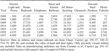
VALUE OF CAPITAL FOR SELECTED UTILITIES AND MANUFACTURING INDUSTRIES (millions of 1929 dollars)

Sources:

Data on utilities and steam railroads are from Ulmer, Capital, pp. 256–57, 320–21, 374–75, 405–06, and exclude the value of land and land rights. Only privately owned utilities are included. Data on manufacturing industries are from Creamer et al., Capital, pp. 241–47, and include factories with annual value of output of $500 or more.

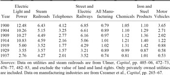
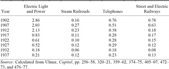
Because quasi-rent is the difference between the value of fixed capital and its value in the best alternative use, the value of an electric utility's fixed capital is an upper bound to the size of appropriable quasi-rent. Reducing that upper bound requires determining what the value of that capital would have been had a utility become unable to provide the services for which that capital was originally acquired. In the case of electric utilities, some of the capital equipment, generators, transformers, land, etc., would have at least partial scrap value. A considerable amount of capital would have virtually no scrap value. This would include the entire distribution system and much of the infrastructure in such buildings as generating stations and substations. The capital of an electric utility was not very mobile. It seems reasonable to assume that appropriable quasi-rent was a large proportion of the capital's value in its intended use. Available descriptive measures show the importance of the value of capital in the early electric utility. This is shown by three tables providing data for the electric utility industry and comparison industries: total value of capital (Table 1), capital output ratios (Table 2), and the ratio of gross investment to total revenue (Table 3).

Table 2

CAPITAL OUTPUT RATIOS FOR SELECTED UTILITIES AND MANUFACTURING INDUSTRIES

Sources:

Data on utilities and steam railroads are from Ulmer, Capital, pp. 405–06, 472–73, 476–77, 482–83, and exclude the value of land and land rights. Only privately owned utilities are included. Data on manufacturing industries are from Creamer et al., Capital, pp. 265–67.

The value of capital invested in the electric power industry was large, but it is when that measure is compared to other economic measures that the potential importance of quasi-rents becomes clear. As shown in Table 1, the total value of capital in electric light and power was less than total capital in steam railways or in total manufacturing. Nevertheless, in 1904 it was a billion 1929 dollars, and for the years shown it was always comparable to the value of capital in the chemical industry. In the earlier years, the value of capital in electric utilities was about one-third that in the iron and steel industry, but was growing faster and eventually exceeded the value of capital in iron and steel. Table 2 shows that electric utilities had much larger capital output ratios than other industries. During the time when most states adopted commission regulation for electric utilities (1914 and before), the capital output ratio for electric utilities was approximately double that of railroads and between seven and eight times that of the iron and steel industry. This very high capital output ratio suggests that capital costs (and, thus, quasi-rents) were a relatively large portion of total costs. Table 3 shows the extent to which the electric power industry was continually dependent on outside investors and creditors. It was not until the year 1915 that the value of electric utility output exceeded total gross investment.Footnote ²³ For the period when most states enacted commission regulation, electric utilities were regularly spending more each year than they received in total revenue, dramatic evidence of the importance of capital (and of the utilities' growth). These data are consistent with the presence of large quasi-rents in the electric utility industry. Did these quasi-rents lead to corrupt practices involving utilities and municipal officials?

Table 3

RATIO OF GROSS INVESTMENT TO VALUE OF OUTPUT: SELECTED YEARS

Source:

Calculated from Ulmer, Capital, pp. 256–58, 320–21, 359–62, 374–75, 405–07, 472–73, and 476–77.

CORRUPTION AND REFORM

The historical record abounds with cases of corruption that arose when utilities had to secure and keep municipal franchises. Many of the examples involved gas, traction, and water utilities, which had been around longer and were larger at the turn of the century than electric utilities. The muckraker Lincoln Steffens cited corruption involving franchises in St. Louis, Philadelphia, Pittsburgh, and Chicago.Footnote ²⁴ San Francisco had a dramatic trial starting in 1906 involving graft, franchises, and “Boss” Ruef.Footnote ²⁵ Similar cases also appear in the historical record of Grand Rapids.Footnote ²⁶ In Chicago, corrupt aldermen created new franchises for the sole purpose of extorting existing franchise holders.Footnote ²⁷ All of these are cities for which the historical record is particularly rich; similar corruption was undoubtedly occurring in many, if not most, other U.S. cities where the record is sparser.Footnote ²⁸ Some in the Progressive Movement, which was active at this time, became sensitive to the corruption that often arose from the interaction between politics and business interests.Footnote ²⁹ Many felt that the primary source of corruption in municipal government was its relationship with privately owned utilities:

The issue of utility or municipal corruption led many Progressive reformers to advocate that utilities be put under municipal ownership, although commission regulation came to be seen as an acceptable alternative. Municipal ownership may seem a strange solution to the problem of corruption involving municipal officials because such an arrangement certainly offered opportunities for corrupt behavior such as supplier kickbacks, employment as reward for political favors, and so on. It would be more difficult, however, for a municipal official to appropriate the quasi-rent of a utility owned by the municipality than one privately owned. Accountability for poor service would more clearly lie with municipal officials, who might hesitate to take actions that could alienate the sources of credit even a municipality would require to own an electric utility, and the opportunity to openly appropriate quasi-rents for public benefit would be lost. Because of the differences in the scales of the production and use of electricity, the vertical integration Williamson argued arose from transaction-specific capital was not possible.Footnote ³¹ Municipal ownership was the closest feasible approximation.Footnote ³²

Whether utilities should be privately owned or municipally owned became an issue in many elections of the time, including both Milwaukee and Atlanta in 1898,Footnote ³³ Cleveland and Toledo in 1903,Footnote ³⁴ New York in 1905,Footnote ³⁵ and Atlanta again in 1906.Footnote ³⁶ It was a perennial concern in Chicago elections, arising in 1902, 1903, and 1905.Footnote ³⁷ Utility ownership was an issue in statewide elections in Massachusetts and Ohio in 1905.Footnote ³⁸

In 1905 the National Civic Federation undertook a well-publicized investigation into the question of whether it was preferable for utilities (electric, gas, tramways, and water) to be owned and operated by private companies or by government. The federation was a Progressive-Era organization that brought together leaders of industry, commerce, and labor, and had achieved some success achieving conciliation in labor disputes.Footnote ³⁹ A committee of 21 individuals was chosen to be evenly divided between those who entered the task favoring municipal ownership, opposing municipal ownership, and having no opinion. The committee, with great fanfare, set out on their two-year task by visiting utilities operating under both forms of ownership in the United States and in Great Britain. In 1907 the committee issued a ponderous report occupying three volumes and nearly 2,500 pages. Different portions of the report were written by different individuals, none of whom appear to have altered positions held at the beginning of the study. The committee agreed that water utilities should be owned by the municipality, but they came to no agreement on the ownership issues for the other utilities. Competition, however, was unanimously rejected as a desirable regulator for all utilities. Municipal ownership or state government price regulation were the only feasible options: “the question is whether it is better to regulate or to operate.”Footnote ⁴⁰ A 1913 editorial in the Wall Street Journal referred specifically to the problems of municipal corruption and “holdup” as reasons for supporting the creation of state utility commissions.Footnote ⁴¹

State regulatory commissions date back at least to the first few decades of the nineteenth century, but the power to regulate rates first appeared with the passage of the “Granger Laws” in the 1870s that created commissions with the power to set the rates of railroads and other businesses.Footnote ⁴² These commissions attracted the attention of courts, including the Supreme Court, whose decisions were to have substantial control over the form that state commission regulation ultimately took. For the present discussion, the most important was Smyth v. Ames, a case that involved an 1893 Nebraska law establishing a commission with the power to order a reduction of railroad rates.Footnote ⁴³ That decision, based on the Fourteenth Amendment (originally designed to protect the rights of freed slaves from abusive state laws), defined the enduring basic principles under which rate regulation has operated to the present. Regulated rates that denied a regulated company from receiving a “fair” return on the “fair value” of its invested property were found to violate the company's constitutional right to due process and equal protection under the law.

The decision opened a large number of issues that had to be decided before an administrative system could be developed that satisfied them.Footnote ⁴⁴ For a number of years, the orders of the early regulatory commissions were so often effectively challenged in court as to have made them meaningless, and it is not clear that railroads were successfully regulated before utilities.Footnote ⁴⁵ The administrative procedures eventually developed to survive judicial scrutiny have resulted in a system that does not lack serious informed criticism. As difficult as the court's principle has been to apply in practice, its goal is clear: the protection of quasi-rents. The requirement that a utility receive a fair return on the value of its investment will prevent the value of that investment from declining as a result of regulatory action. The system might (or might not) facilitate the acquisition of monopoly rents, but it gives protection of quasi-rents the status of a constitutional right, with the full power of state and federal courts to enforce that right.

Approximately three months after the decision in Smyth v. Ames, Samuel Insull, then the president of the National Electric Light Association, the nation's primary electric utility trade organization, advocated rate regulation in a major address at an annual meeting of the member utility companies.Footnote ⁴⁶ His discussion of this topic began with a reference to the “agitation” for municipal ownership (although this issue was relatively quiet at that time compared to what it soon would be). He did not specifically mention corruption, but he was concerned about the risk of the appropriation of quasi-rents and its long-run impact on utilities and their customers:

Insull went on to argue that the least expensive service would be provided if electric utilities were granted exclusive franchises and subject to regulation designed to set prices equal to costs plus a reasonable profit. This, he argued, would lower costs of service primarily because the increased confidence of investors would lower interest rates to the utility.Footnote ⁴⁸ He then advocated that municipalities should be prevented from going into competition with privately owned utilities, but they should have the absolute right to purchase a private utility at a fair price and take over operation if there were unhappiness over the service the private utility offered. This feature was eventually incorporated into the regulatory statutes of several states. Insull's position was not immediately accepted by the member utilities of his trade group. Nevertheless, the idea that regulation and municipal ownership were alternative solutions to the problem of utilities continued to gain traction.Footnote ⁴⁹ Unlike state regulation, municipal ownership of electric utilities never came to dominate the U.S. electric power industry.Footnote ⁵⁰

QUASI-RENTS AND THE TIMING OF STATE REGULATION

Did quasi-rents affect the decision to adopt state regulation? If so, in each year, those states with higher quasi-rents would have had a higher probability of accepting regulation. A discrete-time hazard model was used to test this relationship, and the results are generally consistent with the position that higher quasi-rents did increase the probability of a state's adopting regulation, although the inclusion of average revenue, a measure previous studies have found relevant, does raise questions about that relationship. This approach does not, however, directly address the apparent synchronicity in a state's adoption of regulation. An explanation consistent with the hypothesis that quasi-rents and corruption were responsible for regulation could be partially based on the observation that this was the time period in which municipal utilities first became important. No enterprises prior to utilities had the characteristic of heavy up-front capital investment that resulted in large appropriable quasi-rents and the opportunity this situation created for municipal corruption.

The data used in this analysis were grouped by the time periods defined by the publication of special quinquennial census reports on electric industries. Thus, data were collected for the years 1902–1937 in five-year intervals. Those states that had not achieved statehood by 1937 (Alaska and Hawaii) were not included. Arizona, New Mexico, and Oklahoma were included only after they became states (1912, 1912, and 1907, respectively). For privacy reasons, the census reports sometimes combined states not combined in previous years. States combined with other states were dropped from the analysis. Data for the District of Columbia were always combined with one or more states and were dropped from the analysis. No states adopted regulation in the five-year periods following 1922 and 1927. The data for these years were dropped from the estimation and simulation, but are included in the table of summary statistics.Footnote ⁵¹

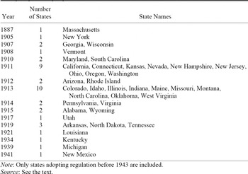
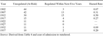
Table 4 shows the year in which regulation was adopted by those states that had done so before 1943.Footnote ⁵²Table 5 shows the hazard rate associated with each time period used in the analysis. The first column shows the number of states that had not adopted regulation by the end of the census year. The second column shows the number of those states that adopted regulation during the following five years; the hazard rate is the ratio of these two. The table shows considerable variation in the hazard rate. Of the states that had not adopted regulation by the end of 1912, 52 percent had done so between 1913 and 1917. By contrast, no states adopted regulation in the periods following 1922 and 1927.

EMPIRICAL ESTIMATION: DESCRIPTION OF VARIABLES

For the purposes of this study, the most important independent variable measures the size of the quasi-rent for all privately owned electric utilities in a state. New regulatory commissions were given authority over several utilities at the same time, and comparable measures of the size of quasi-rent for other utilities would have been desirable but are not included.Footnote ⁵³

Table 4

YEAR OF ESTABLISHMENT OF STATE ELECTRIC REGULATORY COMMISSIONS

Note:

Only states adopting regulation before 1943 are included.

Source:

See the text.

A direct measure of utility quasi-rent is not possible. As discussed above, a measure of total investment would be an upper bound of the size of quasi-rent. If electric utilities in different states were similar in terms of each one's mix of invested capital, and if all utilities were in a similar position with regard to their access to markets for scrap capital, the proportion of total invested capital made up by quasi-rent would be fairly uniform, and the upper bound, value of total capital, should be a good relative measure of quasi-rents. In all but the last two reports, the census provided for each state a measure of the value of land and capital belonging to electric utilities, but its accuracy is questionable. The reports often acknowledged problems with these data because, among other things, electric utilities of the time did not use uniform methods of accounting.Footnote ⁵⁴ In lieu of any estimated value, total generating capacity (kilowatts) of all private utility-owned generators was used. During the early days of electric power, rapid advances were made in the technology of generating equipment that would have caused declines in the real cost of a kilowatt of generating capacity. In such a situation, the total generating capacity might be more closely related to the true economic value of the entire generating plant at that point in time than would accounting measures based on original cost.Footnote ⁵⁵ Total generating capacity is available for all years and is likely to be accurate at measuring what it purports to measure. In order to adjust for the differences in state size, total population and urban population for each state were collected from the decennial census of population, and values for the years of the quinquennial censuses of electric power were calculated by constant growth rate interpolation. Because electric utilities were almost exclusively an urban phenomenon during this entire period, generating capacity was divided by urban population rather than total population.Footnote ⁵⁶

Table 5

OBSERVED HAZARD RATE

Source:

Derived from Table 4 and year of admission to statehood.

Four independent control variables were also included in all models. The first was designed to measure the importance of industrial electricity use. Value added in manufacturing was obtained from census reports (initially reported only in the decennial census, but later reported biennially). Constant growth rate interpolation was used here when needed to obtain values for the observation years. Because industry existed primarily in urban areas at this time, this value was also adjusted by dividing by the state's urban population. The expected impact of a relatively large proportion of a state's electricity being used for industrial, rather than residential, uses is unclear. Industrial users of electricity, unlike residential users, had a close alternative to electricity provided by an electric utility: the firm could generate the electricity itself for its own use. Significant amounts of industrial electricity were self-generated during this period.Footnote ⁵⁷ This alternative should have resulted in higher demand elasticity for electricity by industrial rather than by residential users, a characteristic that would have reduced the size of potential monopoly rents. If the acquisition of monopoly rents were the primary motivation for the adoption of state regulation, the proportion of electricity used for industrial rather than residential purposes should have been inversely related to the probability of a state's adopting regulation. Industrial users should have, nevertheless, been concerned about the corrupt appropriation of utility quasi-rents. These industries may have themselves been potential victims of corrupt officials and therefore would have had an interest in reducing a climate of corruption. If industries had had more political influence than ordinary residential users, their involvement would have had a positive overall effect on the probability of a state's deciding to implement state regulation of electric utilities.

The second independent control variable was designed to measure the proportion of the population who would have been concerned about utilities and corruption, that is, the proportion of the population who were customers of an electric utility or who felt they might soon become customers. Because, as noted above, electric utilities operated essentially only in urban areas, this was measured by the proportion of the total population living in those areas.Footnote ⁵⁸ The adoption of regulation required action by the state legislature whose members would have either rural or urban constituents or a combination of both. The higher the proportion of those constituents who felt that regulation of utilities could reduce municipal corruption, the more likely such action would be undertaken. If, on the other hand, regulation had been sought primarily by utilities seeking to acquire or maintain monopoly rents, surely rent-seeking behavior among state legislators would have been more effective on those whose constituents were unconcerned about the issue. The proportion of the population personally involved with electric utilities would then have been negatively related to the probability of a state's adopting regulation.Footnote ⁵⁹

A third independent variable was designed to capture any effect that a governing party might have had on the probability of regulation. Savitski found that the presence of a Republican governor reduced the probability of a state's adopting regulation, presumably reflecting that party's relative probusiness ideology and consequent resistance to government control over a privately owned company. I have accepted Savitski's hypothesis about Republicans, but used a slightly different measure. Each state was categorized for each year by the party holding the governorship.Footnote ⁶⁰ For the period after the year of the observation, either through the next census year or through the year in which state regulation was adopted (whichever was shorter), the proportion of years in which the state was governed by a Republican was determined.

The fourth independent variable was designed to determine whether the decision of a state to adopt state regulation was affected by the adoption of regulation in an adjacent state in either the same or a previous period. The dummy variable was coded “one” for those states in which an adjacent neighboring state had adopted regulation either previously or in the following five years. This effect is sometimes known as “contagion.”

In addition to these four variables, three other independent variables were included in some of the models. Two of them were designed to measure the extent to which a state's electric utilities were municipally owned. As noted above, municipal ownership was seen as a way of combating corruption by reducing the opportunities to appropriate quasi-rent through vertical integration. Those states with a large degree of municipal ownership would thus have had fewer problems with corruption than states with little municipal ownership. The inclusion of measures of municipal ownership, however, can be expected to reduce the precision with which the coefficients of other independent variables, particularly the measure used for quasi-rents, can be estimated. A degree of multicollinearity can be expected for two reasons: to the extent that municipal ownership and regulation were substitute policy responses to the problem of the appropriation of quasi-rents, the same factors affecting the decision to adopt state regulation would also have affected the extent of municipal ownership. In addition, the measure of quasi-rents I have employed is the ratio of private generating capacity to urban population. A state in which a significant proportion of utilities were municipally owned could be expected, ceteris paribus, to have a lower ratio of privately owned generation per urban population. Models were therefore estimated with and without one of these independent variables.

Two measures of the importance of municipal ownership are reported because of the surprising difference in their results. One measured the proportion of a state's generating capacity (kW) that was owned by municipally owned utilities. The other measured the proportion of a state's total generation (kWh) produced by municipally owned utilities. As would be expected, the correlation between these two measures was very high.Footnote ⁶¹ Yet the variations in the results in using one rather than the other were both different and interesting enough that both are reported.

The last independent variable measured the average revenue for private utilities in the state, a popular variable in other studies.Footnote ⁶² Its interpretation has always been that it measures price level: utilities with higher average revenue charge, on average, higher prices. Despite this tautology, the interpretation of average revenue is more complex because utilities have always engaged in price discrimination depending on the characteristics of the user (residential versus industrial, for example). This means the price faced by any actual electricity user may differ substantially from average revenue.Footnote ⁶³

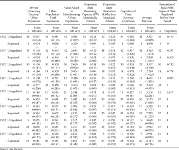
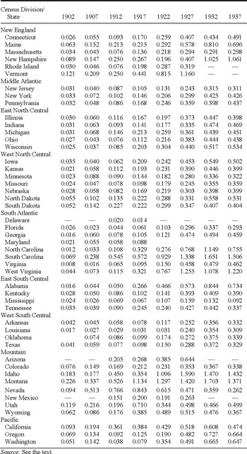
Table 6 provides summary statistics for the independent variables by year for both those states that had not yet adopted state commission regulation and those that had. In 1902 only a single state (Massachusetts) already had commission regulation, and it had a lower value for the ratio of generating capacity to urban population than the average of those states that had not yet adopted regulation. By 1907 three other states (Georgia, New York, and Wisconsin) joined Massachusetts, and the average ratio of generating capacity to urban population was still lower for those four states than for states not yet under commission regulation. Once a larger number of states adopted regulation, this relationship changed, and the regulated states had higher ratios of generating capacity to urban population than did the unregulated states. Furthermore, the differences in the two proportions increased in every time period except for 1932, when it decreased slightly from the difference in 1927. This pattern is consistent with Samuel Insull's expectation that regulation would reduce the fear of investors, easing the ability of utilities to obtain funds. Value added in manufacturing per urban resident was consistently higher for regulated than for unregulated states. The difference increased until 1932, when it declined and then partially rebounded in 1937. The negative impact of the Great Depression on manufacturing for both categories of states was likely responsible for the narrowing of the difference. The proportion of a state's population that was urban was always higher for states with regulation than for those without, although the difference continually fell. Average revenue was higher in Massachusetts in 1902 than in the other states. After that, utilities in states that were regulated had lower average revenue than states without. Average revenue fell overall and faster in regulated than unregulated states until 1917, after which the gap in average revenue declined in each period. For both measures of municipal ownership, unregulated states had higher levels than regulated states. The gap between regulated and unregulated states increased continuously until 1917 and then fluctuated with a larger gap in the 1932 and 1937 periods, perhaps partially reflecting an attitudinal change during the New Deal. Regulated states had higher levels of Republican governorships in the period through 1917 and in 1932 and lower levels in other years. The monotonic increase in the proportion of states with regulation caused a continual increase in the proportion of states with a regulated neighbor. This proportion was never higher for unregulated than for regulated states. Table 7 shows the available data on private generating capacity by state and year.

Table 6

SUMMARY STATISTICS FOR ALL STATES

Source:

See the text.

ESTIMATION RESULTS AND DISCUSSION

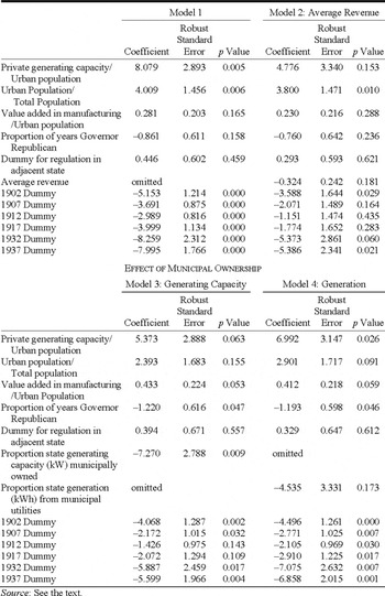
Table 8 presents the results of four different pooled logit estimations including year dummies.Footnote ⁶⁴ Model 1 omits average revenue and measures of municipal ownership. Model 2 includes average revenue but not measures of municipal ownership. Models 3 and 4 include each of two measures of municipal ownership but exclude average revenue. The binary dependent variable was coded one if that state adopted regulation in the following five years. For example, an observation for an individual state for the year 1917 would have the dependent variable coded one if the state adopted regulation in the period from 1918 through 1922, and zero otherwise. Only states that had not yet adopted regulation were included; once a state adopted regulation, it was dropped from the data used for estimation for later years.

Table 7

STATE PRIVATE GENERATING CAPACITY/URBAN POPULATION BY CENSUS DIVISION

Source:

See the text.

The estimated coefficient for the ratio of privately owned generation to urban population is positive in all estimations, and significant in all but Model 2. As discussed below, I believe Model 1 gives the most accurate indication of that effect. A positive relationship supports the hypothesis that higher levels of appropriable quasi-rent increased the probability of a state's adopting regulation.

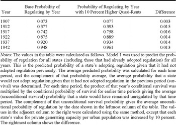
Even if the amount of potentially appropriable quasi-rent significantly increased the probability of a state's adopting regulation, was the magnitude of that effect meaningful? Table 9 attempts to quantify that effect by estimating the average impact on the average cumulative probability of regulation that would have been predicted by Model 1 had a state's level of private generating capacity per urban population been 10 percent higher than it actually was. These can be interpreted as follows: The probability of a state's having adopted regulation on or before 1917 was 0.742. With a 10 percent higher level of private generating capacity per urban population, that probability would have been 0.758. The difference, 0.016, is modest, but large enough to be meaningful. This is an indicator of the magnitude of the effect of marginal differences among the states, and is not inconsistent with corruption being the primary impetus for the adoption of regulation in all states.

The results in all models except Model 2 are quite similar. The inclusion of average revenue caused the largest changes in the estimated partial effects of quasi-rents and all other independent variables. Compared to Model 1, the coefficient for the measure of quasi-rents fell in magnitude about 40 percent and changed from being highly significant to insignificant. It retained, however, its positive sign. The coefficients for all the other independent variables also fell in magnitude and became less significant, but their signs were also unchanged. The coefficient on average revenue is negative but not significant (at the 10 percent level). A fuller discussion of the meaning of the result of including this variable appears below, after discussion of the results for the other independent variables.Footnote ⁶⁵

Table 8

ESTIMATION RESULTS

Source:

See the text.

Table 9

EFFECT OF 10 PERCENT HIGHER QUASI-RENT ON CUMULATIVE PROBABILITY OF REGULATION

Notes:

The values in the table were calculated as follows. Model 1 was used to predict the probability of regulation for all states (including those that had already adopted regulation) for all years. This is the predicted probability of a state's adopting regulation given that it had not adopted regulation previously. The average predicted probability was calculated for each time period, and the complement of that probability average, the average probability that a state would not adopt regulation given that it had not adopted regulation in the previous period (survival) was determined. For each time period, the product of that year's conditional survival was multiplied by the conditional probability of survival for earlier time periods giving the average (unconditional survival) probability that a state would have remained unregulated by that time period. The complement of that unconditional survival probability gives the average unconditional probability of regulation by the date shown in the leftmost column of the table. The values in the adjacent column to the right were calculated using the same method, except that each state's value for private generating capacity per urban population was increased by 10 percent. The rightmost column shows the difference.

The results of the formulation omitting average revenue are strongly supportive of the hypothesis that large quasi-rents increased the probability of regulation. Larger amounts of privately invested capital (and, therefore, quasi-rents) were significantly related to an increased probability that state regulation would be adopted. The inclusion of measures of the importance of municipal ownership, as expected, reduced the significance of this variable. Nevertheless, it remained significant at the 10 percent level, the sign on the coefficient was unchanged, and the magnitude of the estimated coefficient was modestly reduced.

The positive estimated relationships between “the probability of regulation” and both “value added over urban population” and “proportion of the population living in urban areas” were always positive, but the level of significance showed some sensitivity to the precise set of other independent variables. Positive relationships, as discussed earlier, are both consistent with the hypothesis that regulation was adopted to protect quasi-rents and inconsistent with the dominant hypothesis that it was adopted to enable utility companies to obtain higher monopoly rents.

The coefficient on the proportion of years in which a state's governor was Republican was always negative, but was significant only when one of the measures of municipal ownership was included. A negative coefficient is consistent with Savitski's hypothesis that Republicans were resistant to state regulation. The positive estimated coefficient for the dummy variable measuring whether a neighboring state had either adopted regulation or would adopt regulation in the next five years is consistent with a “contagion” effect, but the level of significance is very low in all models.

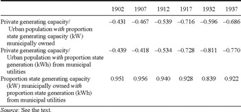
The two measures of municipal ownership both had negative estimated coefficients, consistent with the positions taken by Troesken, and Troesken and Rick Geddes, that municipal ownership reduced the likelihood of the appropriation of quasi-rents or with the very similar position that municipal ownership was an alternative to state regulation. It is a little puzzling that the two measures of municipal ownership had effects on the estimation that were so different. For the measure of the proportion of total generating capacity (kW) owned by municipal utilities, the estimated coefficient was highly significant. For the measure of the proportion of state generation (kWh) produced by municipal utilities, the estimated coefficient was insignificant. Although the inclusion of either measure reduced the significance (and estimated magnitude) of the coefficient on privately owned capital per urban population, the effect of the measure based on generating capacity was greater than that based on generation. As expected, the correlation between those two measures (shown in Table 10) was very high. There also was little difference in the correlations between either of these measures and the measure of quasi-rent.

What explains the effect of the inclusion of the average revenue variable? Its inclusion does not reverse conclusions about the other independent variables since the signs of none of the other coefficients changed. It does, however, raise the question of whether the apparent relationship might be random. Although average revenue is not itself significant (at the 0.10 level), its inclusion sharply reduces the significance of all other explanatory variables, including the year dummies. This result is suggestive of multicollinearity. Average revenue may itself be related to the level of quasi-rents. The strongest simple correlations with average revenue are with value added over urban population (−0.32) and generating capacity over urban population (−0.20). When average revenue is regressed against all the other independent variables, both value added over urban population and generating capacity over urban population have negative coefficients that are highly significant (better than 0.01). Some of the year dummies are also significant. The R ², however, is only 0.23, indicating that other factors are responsible for most of the variation in average revenue.

Table 10

SIMPLE (PEARSON) CORRELATIONS AMONG SELECTED INDEPENDENT VARIABLES (ESTIMATION SAMPLE)

Source:

See the text.

INTERPRETATION OF THE EFFECT OF AVERAGE REVENUE

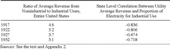
If average revenue were interpreted as a measure of price, its negative coefficient would be supportive of the conclusion reached in many previous studies that regulation was enacted in the interests of utility companies and against the interests of consumers. Could this accepted interpretation of average revenue measuring price be incorrect? Could the presence of price discrimination have caused average revenue to be less a measure of the level of prices than the mix of electricity users? Unfortunately, data permitting a direct examination of this issue are not available until 1917, after most states had adopted regulation. The data available after 1917 show that industrial customers faced much lower prices for electricity (per kWh) than did nonindustrial users. Furthermore, average revenue for a state was heavily affected by the proportion of electricity in that state that was used by industrial customers.

Table 11

AVERAGE REVENUE AND INDUSTRIAL VS. NONINDUSTRIAL SALES

Sources:

See the text and Appendix 2.

There are two explanations for the lower prices charged industrial users. First, it was cheaper for the utility to provide electricity to industrial than to residential customers. The amount of distribution equipment per unit of energy supplied would have been lower for those consuming relatively large amounts at a single location. Even more important, industrial electricity use tended to occur off-peak because system peaks during that period (prior to at least 1921) were primarily determined by residential customers using lights in the early evening.Footnote ⁶⁶ Second, as noted previously, industrial users would have had much higher price elasticity of demand than nonindustrial users because the former had a close substitute for utility-supplied electricity. If prices tended to be above marginal cost, profit-maximizing price discrimination would have caused that difference to be smaller for industrial than for other customers.

Average revenue and kWh usage for both industrial and nonindustrial electricity users were obtained for the years 1917, 1922, 1927, and 1932. Table 11 was derived from these data.Footnote ⁶⁷ The first column of Table 11 provides the ratio of the average revenues from nonindustrial to industrial users for the entire United States. The second column shows the state-level correlation between average revenue and the proportion of utility supply that went to industrial users. It is unfortunate that two of the years (1917 and 1932) were ones in which the U.S. economy was undergoing unusual stresses. Nevertheless, the high correlation coefficients, especially for 1917 and 1922, support the hypothesis that average revenue is not simply a proxy for overall prices but may also (primarily?) have captured the relative importance of industrial electricity use. This is consistent with large industrial electricity usage positively affecting the probability of the adoption of state regulation. The independent variable measuring a state's manufacturing value added per urban population was designed to capture the effect of the relative size of industrial electricity use. It does not, however, distinguish the differing effects that may have been attached to industrial users who were customers of utilities versus industrial users who self-generated the electricity they used.