4.1.1. Validity of the formulation

The physics-based rationale presented in § 4.1 uses the following assumptions: (i) the Mach numbers are small; (ii) there is a time interval for which the acoustic field is time-periodic in the relevant region wherein it reaches its far-field form (1.4); (iii) there is a region covering the wavelength scale where the velocity field is as induced by a point vortex. Condition (i) is ensured by (2.5). For condition (iii), we need

(4.2a,b)\begin{equation} \delta = k r_* \ll 1, \quad \varepsilon = 1 / (k L) \ll 1. \end{equation}

For condition (ii), the incident wave has to overcome the region $r / r_F = O(1)$ long before time-periodicity is destroyed, which might be possible owing to: (a) the viscous diffusion of the vortex at times $O(r_*^2 / \nu _\infty )$; (b) the acoustic instability of the Rankine vortex at $O(r_*^6 c_\infty ^4 / \varGamma _*^5)$ (see Kopiev & Leontiev (Reference Kopiev and Leontiev1983) and Kop'ev & Chernyshev (Reference Kop'ev and Chernyshev2000), § 3.2); (c) the nonlinear self-convection of the wave at $O(\omega ^{-1} / a)$. Using the evaluation (5.9) we need to assume the following relationships between dimensional spatial scales:

(4.3)\begin{equation} \left.\begin{gathered} \max \left(\nu_\infty / c_\infty,\ \varGamma_* / c_\infty\right) \ll r_* \ll \lambda \ll L \ll r_F = O(L^2 / \lambda), \\ L^2 / \lambda \ll c_\infty (t - t_0) \ll \min \left(r_*^6 c_\infty^5 / \varGamma_*^5,\ r_*^2 c_\infty / \nu_\infty,\ \lambda / a\right). \end{gathered}\right\} \end{equation}

In terms of dimensionless variables, the requirement that $r_F / c_\infty$ is much shorter than the three temporal scales leads to additional restrictions for the small parameters (2.5), (4.2):

(4.4a–c)\begin{equation} M^5 \ll \delta \varepsilon^2, \quad M \ll \mbox{Re} \,\delta \varepsilon^2, \quad a \ll \varepsilon^2, \end{equation}

where $\mbox {Re} = \varGamma _* / \nu _\infty$. The first condition represents the restriction owing to instability, the second diffusion and the third nonlinear convection.

To apply perturbation theory, we also require the Born approximation (2.18). Equation (3.1) with the source (4.11), (4.10) suggests that the sufficient condition for its validity is high-frequency scattering, meaning that the angular frequency of the incident wave is high compared with the maximum angular velocity of the flow, i.e.

(4.5)\begin{equation} M / \delta = \varGamma_* / (2 {\rm \pi}\omega r_*^2) \ll 1. \end{equation}

The actual sufficient condition seems to be less rigorous than (4.5), though more rigorous than (2.5b):

(4.6)\begin{equation} M \ll \delta \quad \mbox{or} \quad M \ll 1, \quad M \neq \delta / n + O(\delta^2), \quad n \in \mathbb{Z}. \end{equation}

The latter restriction is related to fact that the Rankine vortex is able to emit sound on its eigenfrequencies $n M / \delta$, where $M / \delta$ is the dimensionless angular velocity in the region $r < \delta$. The same is likely for the case of the vortex (4.10), as it is similar to the Rankine vortex. When the angular frequency of the incident wave is close to one of the eigenfrequencies, the resonant amplification makes the scattered field comparable to the incident field (Sozou Reference Sozou1990; Ford & Smith Reference Ford and Smith1999; Kopiev & Belyaev Reference Kopiev and Belyaev2010).

5.1.1. Representation using the Fourier transform

First, it is useful to derive an exact representation of the solution to the general well-posed RP that does not contain non-elementary functions. Let us apply the two-dimensional Fourier transform

(5.1a,b)\begin{align} \widehat \rho_{11} (\boldsymbol{K}) = \frac {1}{2 {\rm \pi}} \int_{\mathbb{R}^2} \rho_{11} (\boldsymbol{r}) \exp({- \mathrm{i}\boldsymbol{K \cdot r}}) \,\mathrm{d}^2 \boldsymbol{r},\quad \widehat q_{11} (\boldsymbol{K}) = \frac {1}{2 {\rm \pi}} \int_{\mathbb{R}^2} q_{11} (\boldsymbol{r}) \exp({- \mathrm{i}\boldsymbol{K \cdot r}}) \,\mathrm{d}^2 \boldsymbol{r}\end{align}

to the Helmholtz equation (3.1). Owing to the decay condition (3.5),

(5.2)\begin{equation} \frac {1}{2 {\rm \pi}} \int_{\mathbb{R}^2} \nabla^2 \rho_{11} \exp({- \mathrm{i}\boldsymbol{K \cdot r}}) \,\mathrm{d}^2 \boldsymbol{r} ={-} K^2 \widehat \rho_{11}. \end{equation}

Equations (5.1a,b) and (5.2) give

(5.3)\begin{equation} (1 - K^2) \widehat \rho_{11} = \widehat q_{11}. \end{equation}

We extract $\widehat \rho _{11}$ and make the inverse Fourier transform, which gives

(5.4)\begin{equation} \rho_{11} = \frac {1}{2 {\rm \pi}} \int_{\mathcal{C}} \frac {\widehat q_{11} (\boldsymbol{K})} {1 - K^2} \exp({\mathrm{i} \boldsymbol{K \cdot r}}) \,\mathrm{d}^2 \boldsymbol{K}.\end{equation}

The two-dimensional cycle $\mathcal {C} \subset \mathbb {C}^2$ in (5.4) is the plane $\mathbb {R}^2$ deformed to bypass the singular circle $K = 1$, which corresponds to eigensolutions of the Helmholtz operator, appropriately to fulfil the radiation condition (3.4)

(5.5)\begin{equation} \mbox{Re} (\boldsymbol{K}) \boldsymbol{\cdot} \mbox{Im} (\boldsymbol{K}) < 0 \quad \mbox{for}\ \boldsymbol{K} \in \mathcal{C} \ \mbox{near}\ K = 1, \end{equation}

which is equivalent to the causality condition (see § 1). The representation (5.4) with $\mathcal {C}$ observing the rule of bypass (5.5) and the representation (3.6) are equivalent and related to each other by the convolution theorem.

5.1.2. Far-field representation

The source (4.11), (4.12) is localised within the flow region $\varepsilon r = O(1)$. Consequently, in the region of fluid at rest $\varepsilon r \to \infty$ it is possible to use asymptotics (3.7) for Green's function in (3.6), because any of the primitive waves emitted from the important region $\varepsilon r' = O(1)$ overcome the long distance $|\boldsymbol {r} - \boldsymbol {r'}| \gg 1$. The distance is expanded in a power series by $\boldsymbol {r'}$ as

(5.6)\begin{equation} |\boldsymbol{r} - \boldsymbol{r'}| = r - \boldsymbol{\hat{r}} \boldsymbol{\cdot} \boldsymbol{r'} + \frac{(\boldsymbol{\hat{\theta}} \boldsymbol{\cdot} \boldsymbol{r'})^2}{2 r} + O \left(\frac{1}{\varepsilon^3 r^2}\right) \quad \mbox{as}\ \varepsilon r \to \infty. \end{equation}

We need only keep the leading-order term of (5.6) in the denominator of (3.7), but the complete expansion in the exponent.

The greatest possible simplification for the exponent of (3.7) is the linearisation of (5.6) by $\boldsymbol {r'}$, known as the Fraunhofer approximation. It is valid only in the region $\varepsilon ^2 r \to \infty$, the farthest part of the region of fluid at rest. Substituting this into (3.6) and using (3.3b), we obtain the outgoing cylindrical wave (1.4)

(5.7a,b)\begin{equation} \rho_{11} \sim \frac {\exp({\mathrm{i} r - \mathrm{i} {\rm \pi}/ 4})} {\sqrt{r}} f (\theta),\quad \boldsymbol{v}_{11} \sim \boldsymbol{\hat{r}} \rho_{11} \quad \mbox{as}\ \varepsilon^2 r \to \infty, \end{equation}

with the scattering amplitude

(5.8)\begin{equation} f ={-} \mathrm{i} \sqrt{\frac {\rm \pi}{2}}\widehat q_{11} (\boldsymbol{\hat{r}}), \end{equation}

where $\widehat q_{11}$ is the source Fourier transform defined by (5.1b). Its argument $\boldsymbol {\hat {r}}$ reflects the direction of sound propagation in the far field. The solution (5.7a), (5.8) satisfies the radiation condition (3.4) and in the leading-order approximation the Helmholtz equation (3.1), which is homogeneous because of (4.13). This can also be derived from (5.4) by using the multidimensional stationary-phase method (see Fedoryuk Reference Fedoryuk1963).

In the region $\varepsilon ^2 r = O(1)$ we need to keep the quadratic term of (5.6) dependent on $\boldsymbol {r}$, which leads to the breakdown of (5.7). This defines the bound of the far field according to (3.4) as

(5.9)\begin{equation} r_F = \varepsilon^{{-}2}. \end{equation}

Equation (5.9) indicates that the near field $r / r_F = O(1)$, where the scattered field is different from (5.7), is much longer than the flow region. This suggests a multiscale scattering pattern, including in the region of fluid at rest $\varepsilon r \to \infty$.

5.3.1. Far field $\varepsilon ^2 r \to \infty$

The scattering amplitude in the far field can be obtained by direct substitution of (5.13) into (5.8) giving

(5.14)\begin{equation} f = f^{(i)} (1 - \exp({- |\boldsymbol{\hat{r}} - \boldsymbol{\hat{k}}|^2 / 4 \varepsilon^2})) \sim f^{(i)} (1 - \exp({- \theta^2 / 4 \varepsilon^2})), \end{equation}

where

(5.15)\begin{equation} f^{(i)} ={-} \sqrt{2 {\rm \pi}} ~ \frac {\boldsymbol{\hat{r}} \boldsymbol{\cdot} \boldsymbol{\hat{k}}\, \boldsymbol{\hat{z}} \boldsymbol{\cdot} (\boldsymbol{\hat{r}} \times \boldsymbol{\hat{k}})}{|\boldsymbol{\hat{r}} - \boldsymbol{\hat{k}}|^2} = \sqrt{\frac{\rm \pi}{2}} \cos \theta \cot \frac{\theta}{2} \end{equation}

is exactly expression (i) with the singularity for case PWPV, $|\boldsymbol {\hat {r}} - \boldsymbol {\hat {k}}| = 2 \sin (\theta / 2)$.

By the analogous method Berthet & Lund (Reference Berthet and Lund1995) obtained the solution for the case $\varGamma = \exp (- \varepsilon r)$

(5.16)\begin{equation} f = f^{(i)} \frac {|\boldsymbol{\hat{r}} - \boldsymbol{\hat{k}}|^2 / \varepsilon^2} {\sqrt{1 + |\boldsymbol{\hat{r}} - \boldsymbol{\hat{k}}|^2 / \varepsilon^2} (1 + \sqrt{1 + |\boldsymbol{\hat{r}} - \boldsymbol{\hat{k}}|^2 / \varepsilon^2})}, \end{equation}

with the possible substitution $|\boldsymbol {\hat {r}} - \boldsymbol {\hat {k}}| \to \theta$ as in (5.14). However, there was no clear definition of the far field $\varepsilon ^2 r \to \infty$ where (5.16) was valid. Its application to the region that is actually the near field is incorrect and, in particular, leads to a violation of the Helmholtz equation (3.1) in the flow region (see the explanation in § 5.4).

Both (5.14) and (5.16) are regular patterns that peak at small scattering angles so that

(5.17a,b)\begin{gather} f = O(\varepsilon^{{-}1}), \quad |\boldsymbol{U}_{11}| = O(\varepsilon^{{-}1} / \sqrt{r}) \ll 1 \quad \mbox{as}\ \theta / \varepsilon = O(1), \end{gather}

(5.18a,b)\begin{gather}f = O(1), \quad |\boldsymbol{U}_{11}| = O(1 / \sqrt{r}) \quad \mbox{as} \ \theta = O(1), \end{gather}

and match expression (i) at large angles (figure 4), i.e.

(5.19)\begin{equation} f \sim f^{(i)} \quad \mbox{as}\ \theta / \varepsilon \to \infty. \end{equation}

Figure 4.

The scattering amplitude in the far field: expression (i) (5.15) for $\varGamma = 1$ (black, dashed); the solution (5.14) for $\varGamma = \exp (- \varepsilon ^2 r^2)$, $\varepsilon = 0.05$ (orange, solid); the solution (5.16) for $\varGamma = \exp (- \varepsilon r)$, $\varepsilon = 0.05$ (dark green, solid).

5.3.2. Region of geometrical acoustics $\varepsilon ^2 r \to 0$

The scattered field in the region of geometrical acoustics includes both the radiation component and the distortion component defined in § 2.1, i.e.

(5.20)\begin{equation} \boldsymbol{U}_{11} = \boldsymbol{U}_{11}^r + \boldsymbol{U}_{11}^d. \end{equation}

We remember that in the far field only the radiation component is present, meaning that $\boldsymbol {U}_{11}^d \to 0$ as $\varepsilon ^2 r \to \infty$. We will use the fact that the amplitude and phase (2.21a,b) of a uniform plane incident wave (4.8) are, respectively,

(5.21a,b)\begin{equation} A_0 = 1, \quad \varphi_0 = \boldsymbol{\hat{k} \cdot r}, \end{equation}

whereas the amplitude change and phase shift (2.22a,b) owing to scattering are given by

(5.22a,b)\begin{equation} A_1 = |\rho_{11}| \cos (\arg \rho_{11} - \boldsymbol{\hat{k} \cdot r}), \quad \varphi_1 = |\rho_{11}| \sin (\arg \rho_{11} - \boldsymbol{\hat{k} \cdot r}). \end{equation}

The radiation component is

(5.23)\begin{equation} \left.\begin{gathered} \rho_{11}^r \sim{-} {\rm \pi}\mathrm{i} \exp({\mathrm{i} r (1 - \theta^2 / 2)}) \frac{\theta}{2} \cos \theta \cot \frac{\theta}{2} \left[\mbox{sgn} (\theta) - \mbox{erf} \left(\frac {\mathrm{e}^{- \mathrm{i} {\rm \pi}/ 4} \sqrt{r} \theta}{\sqrt{2}}\right) \right], \\ \boldsymbol{v}_{11}^r \sim \boldsymbol{\hat{r}} \rho_{11}^r. \end{gathered}\right\} \end{equation}

Within the narrow parabolic region at small angles, it represents the non-decaying field with

(5.24)\begin{equation} |\boldsymbol{U}_{11}^r| = O(1) \quad \mbox{as}\ \sqrt{r} \theta = O(1). \end{equation}

At large angles, (5.23) as well as the far-field solution (5.14) is the outgoing cylindrical wave matching expression (i):

(5.25)\begin{equation} \rho_{11}^r \sim \frac {\exp({\mathrm{i} r - \mathrm{i} {\rm \pi}/ 4})} {\sqrt{r}} f^{(i)} (\theta) \quad \mbox{as}\ \sqrt{r} \theta \to \infty. \end{equation}

The angular ranges of (5.14) and (5.23) are different, each being extrapolated to another region will be narrow compared with its counterpart (see figure 6).

The distortion component is

(5.26)\begin{align} \rho_{11}^d &\sim{-} \mathrm{i} \exp({\mathrm{i} \boldsymbol{\hat{k} \cdot r}}) \int_{- \boldsymbol{\hat{k}} \infty}^{\boldsymbol{r}} \boldsymbol{\hat{k}} \boldsymbol{\cdot} \boldsymbol{v}_{10} (\boldsymbol{r'}) \boldsymbol{\hat{k}} \boldsymbol{\cdot} \mathrm{d} \boldsymbol{r'} \nonumber\\ &= {\rm \pi}\mathrm{i} \,\mathrm{e}^{\mathrm{i} x} \left[2 T \left(\sqrt{2} \varepsilon y, x / y \right) + \frac{1}{2} (\mbox{sgn} (y) - \mbox{erf} (\varepsilon y)) \right], \nonumber\\ \boldsymbol{v}_{11}^d &\sim \boldsymbol{\hat{k}} \rho_{11}^d, \end{align}

where the Owen $T$-function is defined by (A5). It represents a non-uniform plane wave that does not interfere with the incident wave (4.8), giving

(5.27a,b)\begin{equation} A_1^d = 0, \quad \varphi_1^d = \mbox{sgn}(y) |\rho_{11}^d|, \end{equation}

as follows from (5.22a,b). In terms of the alternative definition (2.28), (2.30), the scattered wave corresponds to (5.23), whereas the incident wave corresponds to (4.8a,c) $+ M_\lambda$ (5.26). The latter is a non-uniform plane wave that can be rewritten using (5.21) as

(5.28)\begin{equation} \rho_{inc}' \propto \rho_{01} + M_\lambda \rho_{11}^d \sim \exp [\mathrm{i}(\boldsymbol{\hat{k} \cdot r} + M_\lambda \varphi_1^d (\boldsymbol{r}))]. \end{equation}

The wavefront of (5.28) is retarded in the half-plane $y > 0$, where sound propagates upstream, and advanced in $y < 0$, where sound propagates downstream (figure 5). According to the integral expression in (5.26), the phase shift (5.27b) is proportional to the circulation of the vortex velocity along the straight line from the infinity inlet. Wavefront distortion is localised within the flow region and in the wake behind it such that

(5.29)\begin{equation} |\boldsymbol{U}_{11}^d| = O(1) \quad \mbox{as}\ \varepsilon r \theta = O(1), \end{equation}

and decays exponentially beyond. In the region of fluid at rest where $\varGamma \to 0$, from (5.26) we have

(5.30)\begin{equation} \rho_{11}^d \sim {\rm \pi}\mathrm{i} \,\mathrm{e}^{\mathrm{i} x} \mathcal{H} (x) [\mbox{sgn} (y) - \mbox{erf} (\varepsilon y)] \quad \mbox{as}\ \varepsilon r \to \infty, \end{equation}

where $\mathcal {H} (x)$ is the Heaviside step function, equal to $1$ in the forward direction and $0$ in the backward direction. In the region $\varepsilon y \to 0$, which includes the irrotational flow region $\varepsilon r \to 0$ where $\varGamma \to 1$,

(5.31)\begin{equation} \rho_{11}^d \sim {\rm \pi}\mathrm{i} \exp({\mathrm{i} r \cos \theta}) [\mbox{sgn}(\theta) - \theta / {\rm \pi}] \quad \mbox{as}\ \varepsilon y \to 0. \end{equation}

According to (5.31) the wavefront distortion owing to the velocity field decaying proportional to $r^{-1}$ as $r \to \infty$ is finite, because the longitudinal velocity is proportional to $x^{-2}$ as $x \to \infty$ (see McIntyre (Reference McIntyre2019), figure 2).

Figure 5.

The wavefronts of the incident field defined by (4.8) $x = -10 {\rm \pi}; 0; 10 {\rm \pi}; 20 {\rm \pi}$ (red, dashed) and by (5.26), (5.27b), (5.28) $x + M_\lambda \varphi _1^d = {\rm \pi}n$, $n \in \mathbb {Z}$ (black, solid) in the region of geometrical acoustics $\varepsilon ^2 r \to 0$ for $\varGamma = \exp (- \varepsilon ^2 r^2)$, $\varepsilon = 0.05$ and $M_\lambda = 0.25$.

Figure 6.

Asymptotic regions of the source (filled circle) and the solution presented in figure 10 as $\varepsilon \to 0$ in terms of orders of quantities corresponding to table 1.

To summarise, the scattered field (5.23) $+$ (5.26) beyond the flow region and the wake is the outgoing cylindrical wave matching expression (i),

(5.32a,b)\begin{equation} \rho_{11} \sim \frac {\exp({\mathrm{i} r - \mathrm{i} {\rm \pi}/ 4})} {\sqrt{r}} f^{(i)} (\theta), \quad \boldsymbol{v}_{11} \sim \boldsymbol{\hat{r}} \rho_{11} \quad \mbox{as}\ \varepsilon r \theta \to \infty. \end{equation}

This confirms the suggestion of §5.2 that this region is, in fact, the far field. As the wake in (5.26) is wide compared with the parabolic region in (5.23) (see figure 6), in the intermediate region the distortion component dominates such that

(5.33a,b)\begin{equation} \rho_{11} \sim \rho_{11}^d, \quad \boldsymbol{v}_{11} \sim \boldsymbol{\hat{k}} \rho_{11} \quad \mbox{as}\ \varepsilon r \theta = O(1). \end{equation}

However, only the radiation component contributes to the interference pattern, so that

(5.34a,b)\begin{equation} |\boldsymbol{U}_{11}| = O(1), \quad |A_1| = O(1 / \sqrt{r}) \quad \mbox{as}\ \varepsilon r \theta = O(1). \end{equation}

Within the parabolic region

(5.35a,b)\begin{equation} |\boldsymbol{U}_{11}| = O(1), \quad |A_1| = O(1) \quad \mbox{as}\ \sqrt{r} \theta = O(1). \end{equation}

The discontinuity in the direction $\theta = 0$, which is present in (5.23) as well as in (5.26), vanishes on summation.

The solution (5.23) $+$ (5.31) is precisely expression (ii) for the case PWPV $\varGamma = 1$ that does not decay anywhere. (The corresponding scattered field in terms of the definition (2.30) does not decay only within the parabolic region $\sqrt {r} \theta = O(1)$.) It is valid in the irrotational flow region $\varepsilon r \to 0$ where $\varGamma \to 1$. Moreover, it persists in the region $\varepsilon ^2 x \to 0$, $\varepsilon y \to 0$ including its backward as well as forward part, meaning that the scattered wave does not feel the decay of the flow. Independence of the solution on $\varepsilon$ indicates the region of geometrical acoustics, since the wavelength remains the only spatial scale. Expression (ii) was obtained in equivalent forms by Aharonov & Bohm (Reference Aharonov and Bohm1959, (21) and (23)), Berry et al. (Reference Berry, Chambers, Large, Upstill and Walmsley1980, (14) and (A9)), Sakov (Reference Sakov1993, (23)), Ford & Smith (Reference Ford and Smith1999, (5.7) and (5.11)–(5.12)), Howe (Reference Howe1999, (6), (11), (12), (14) and (17)) and Kopiev & Belyaev (Reference Kopiev and Belyaev2010, (21), (24), (32) and (34)), some of which were related to different variables and some contained misprints.

5.3.3. Near field $\varepsilon ^2 r = O(1)$

The near-field solution at large angles, consistent with the foregoing is the outgoing cylindrical wave matching expression (i), written

(5.36)\begin{equation} \rho_{11} \sim \frac {\exp({\mathrm{i} r - \mathrm{i} {\rm \pi}/ 4})} {\sqrt{r}} f^{(i)} (\theta) \quad \mbox{as}\ \varepsilon^2 r = O(1), \quad \theta / \varepsilon \to \infty. \end{equation}

The solution in the near field $\varepsilon ^2 r = O(1)$ at small angles $\theta / \varepsilon = O(1)$ is obtained only as the single integral (A1), (A4)–(A10) and cannot be unambiguously divided into the radiation and distortion components. Some researchers who used the terminology of (2.28), (2.30) interpreted that the incident and scattered fields could not be separated from each other. Here, the scattered field is rearranged from (5.23) $+$ (5.26) in the region of geometrical acoustics to qualitatively different (5.7a,b), (5.14), (5.15) in the far field. The order of the amplitude is evidently

(5.37)\begin{equation} |\boldsymbol{U}_{11}| = O(1) \quad \mbox{as}\ \varepsilon^2 r = O(1), \quad \theta / \varepsilon = O(1). \end{equation}

5.3.4. Overall pattern

The evaluations in §§ 5.3.1–5.3.3 define four asymptotic regions with different orders of $|\boldsymbol {U}_{11}|$, $|A_1|$, which can be classified by two independent criteria (figure 6 and table 1). The region of geometrical acoustics is included in the near field in this sense. The far field 1a $\cup$ 1b and the near field 2a $\cup$ 2b are exactly the regions predicted by the analysis of the Fourier representation in § 5.2 (compare with figure 2). In addition, the far field and the near field are exactly the regions where the amplitude of the scattered wave $|\boldsymbol {U}_{11}| \ll 1$ and $|\boldsymbol {U}_{11}| = O(1)$, respectively. Note that $\max |\boldsymbol {U}_{11}| = O(1)$, so that the Born approximation remains uniformly valid as required.

Table 1.

Orders of $|\boldsymbol {U}_{11}|$, $|A_1|$, $|\,f|$ in asymptotic regions shown in figure 6.

The solution obtained is reduced to expressions (i) and (ii) for case PWPV $\varGamma = 1$ and an analogue to the solution by Berthet & Lund (Reference Berthet and Lund1995) for the case $\varGamma = \exp (- \varepsilon r)$ in different regions (table 2).

Table 2.

Known expressions that are included in the present solution in different regions (see figure 6).

The real part of the numerical solution obtained using the exact representation (A1), (A4)–(A10) is presented in figure 3(c). In order to visualise the near-field solution in a similar manner to the far-field, it is useful to generalise the scattering amplitude to the complex-valued function dependent on $r$ by

(5.38)\begin{equation} \rho_{11} \equiv \frac {\exp({\mathrm{i} r - \mathrm{i} {\rm \pi}/ 4})} {\sqrt{r}} f(\boldsymbol{r}). \end{equation}

Scattering patterns $|\,f(r, \theta )|$ on various distances $r = \mbox {const}$ within the region of fluid at rest $\varepsilon r \gg 1$ are presented in figures 7–9, including the leading-order solution as $\varepsilon \to 0$ determined in §§ 5.3.1 and 5.3.2 and the numerical solution. As $f (r, - \theta ) = - f (r, \theta )$, only the upper half-plane $0 \le \theta \le {\rm \pi}$ is shown. Peaks at small angles and nulls in the forward $\theta = 0$, transverse $\theta = {\rm \pi}/ 2$ and backward $\theta = {\rm \pi}$ directions are visible. Figure 9(a,c) shows that in practice the region $r < 0.2 \varepsilon ^{-2}$ can be considered as the region of geometrical acoustics, whereas the region $r > 0.5 \varepsilon ^{-2}$ can be considered as the far field. The oscillations appearing in the region of geometrical acoustics (figure 8) reflect the interference of the radiation component (5.23) and the distortion component (5.26).

Figure 7.

Scattering patterns in the far field for $\varGamma = \exp (- \varepsilon ^2 r^2)$, $\varepsilon = 0.05$: the leading-order solution as $\varepsilon ^2 r \to \infty$ (5.14) (black, dashed) and the numerical solution for $\varepsilon ^2 r = 0.5$ (blue, solid) and $\varepsilon ^2 r = 1$ (orange, solid).

Figure 8.

Scattering patterns in the region of geometrical acoustics for $\varGamma = \exp (- \varepsilon ^2 r^2)$, $\varepsilon = 0.05$: the leading-order solution for $\varepsilon r \to \infty$, $\varepsilon ^2 r \to 0$ corresponding to (5.23) $+$ (5.30) (dashed) and the numerical solution (solid) for $\varepsilon r = 2$, $\varepsilon ^2 r = 0.1$ (dark green), $\varepsilon r = 4$, $\varepsilon ^2 r = 0.2$ (red).

Figure 9.

Scattering patterns for $\varGamma = \exp (- \varepsilon ^2 r^2)$, $\varepsilon = 0.05$: the leading-order solution in the far field (5.14) (blue, solid), the leading-order solution in the region of geometrical acoustics corresponding to (5.23) $+$ (5.30) (red, solid), the composite solution corresponding to (5.39) (green, solid) and the numerical solution (black, dashed) for $\varepsilon ^2 r = 0.2$ (a); $\varepsilon ^2 r = 0.3$ (b); $\varepsilon ^2 r = 0.5$ (c).

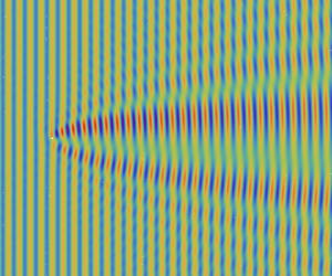
The real part of the total acoustic field $\rho _{01} + M_\lambda \rho _{11}$ calculated using (4.8a) and (A1), (A4)–(A10) for $M_\lambda = 0.5$ (for a clear illustration) is presented in figure 10 (compare with the scheme in figure 6). The sharpest interference pattern $|A_1| = O(1)$ occurs in the parabolic region 2b. The most considerable wavefront refraction is visible in the near field 2a $\cup$ 2b. In the region 2a the wavefronts are similar to those shown in figure 5 (adjusted for the value of $M_\lambda$), while in the region 2b the gap is smoothed out. Similar behaviour can be observed in a physical or numerical experiment if the vortex velocity field exists in a limited region. Examples are water waves patterns corresponding to the cases of small $M_\lambda$ (Vivanco et al. Reference Vivanco, Melo, Coste and Lund1999, figure 2a,b) and numerical patterns (Berthet & Coste Reference Berthet and Coste2003, figures 6, 7). Compare it with results by Berry et al. (Reference Berry, Chambers, Large, Upstill and Walmsley1980, figures 3, 4) for case PWPV and by Coste et al. (Reference Coste, Lund and Umeki1999, figures 2a, 3a) for a similar case in which the refraction was considerable at arbitrarily large distances.

Figure 10.

The total acoustic field $\mbox {Re} (\rho _{01} + M_\lambda \rho _{11})$ given by (4.8a) $+$ $M_\lambda$ (A1), (A4)–(A10) for $\varGamma = \exp (- \varepsilon ^2 r^2)$, $\varepsilon = 0.05$ and $M_\lambda = 0.5$.

The structure of the solution allows us to compose a single expression that will be uniformly valid in the far field $\varepsilon ^2 r \to \infty$, at large angles $\theta / \varepsilon \to \infty$ and in the region of geometrical acoustics $\varepsilon ^2 r \to 0$. For this we use the technique analogous to the method of multiplicative composition, which is commonly used to obtain a uniformly valid solution from matched asymptotic expansions by taking the multiplication of the outer and inner expansions divided by the intermediate approximation (Van Dyke Reference Van Dyke1964, § 5.10). Let us regard the far-field solution (5.7a), (5.14), (5.15) as the outer expansion, the solution in the region of geometrical acoustics (5.23) $+$ (5.26) as the inner expansion and the solution at large angles (5.36), (5.15) as the intermediate approximation. This is possible because in the region 1a the expansions match each other. The composite solution is

(5.39)\begin{align} & \frac {\rho_{11} \rvert_{\varepsilon^2 r \to \infty} \rho_{11} \rvert_{\varepsilon^2 r \to 0}} {\rho_{11} \rvert_{\theta / \varepsilon \to \infty}} \sim {\rm \pi}\mathrm{i} (1 - \exp({- \theta^2 / 4 \varepsilon^2})) \nonumber\\ &\quad \times \left\{ \exp({\mathrm{i} r \cos \theta}) \left[2 T (\sqrt{2} \varepsilon r \sin \theta, \cot \theta ) + \frac{1}{2} \left(\mbox{sgn} (\theta) - \mbox{erf} (\varepsilon r \sin \theta)\right) \right] \right. \nonumber\\ &\quad \left.- \exp({\mathrm{i} r (1 - \theta^2 / 2)}) \frac{\theta}{2} \cos \theta \cot \frac{\theta}{2} \left[\mbox{sgn} (\theta) - \mbox{erf} \left(\frac {\mathrm{e}^{- \mathrm{i} {\rm \pi}/ 4} \sqrt{r} \theta}{\sqrt{2}}\right) \right] \right\}. \end{align}

The expression (5.39) looks more similar to the numerical solution than any of the known leading-order solutions, including in the near field (figure 9b). Apart from the near field, the only region where it leads to the relative error $O(1)$ is the non-relevant neighbourhood of the symmetry axis, where $\rho _{11} \propto \theta$ whereas (5.39) is proportional to $\theta ^3$.

5.3.5. Scattering and momentum-transfer cross-sections

Let us generalise the total scattering cross-section and momentum-transfer cross-section (Pitaevskii Reference Pitaevskii1959) by taking into account the direction of the scattered-wave propagation. In the dimensionless form

(5.40a,b)\begin{equation} \sigma (r) = \int_{-{\rm \pi}}^{\rm \pi} |\boldsymbol{v}_{11}|^2 \boldsymbol{\hat{v}}_{11} \boldsymbol{\cdot} \boldsymbol{r}\,\mathrm{d} \theta, \quad \sigma^* (r) = \int_{-{\rm \pi}}^{\rm \pi} |\boldsymbol{v}_{11}|^2 (\boldsymbol{\hat{v}}_{11} - \boldsymbol{\hat{k}}) \boldsymbol{\cdot} \boldsymbol{r} \,\mathrm{d} \theta, \end{equation}

where $\boldsymbol {\hat {v}}_{11} = \boldsymbol {v}_{11} / |\boldsymbol {v}_{11}|$ is the scattered wave vector, $\boldsymbol {\hat {v}}_{11} \to \boldsymbol {\hat {r}}$ as $\varepsilon ^2 r \to \infty$. In the region of fluid at rest where the wave–vortex interaction is negligible, the scattered energy flux and momentum transfer must be constant,

(5.41a,b)\begin{equation} \sigma (r) \to \sigma_\infty, \quad \sigma^* (r) \to \sigma^*_\infty \quad \mbox{as}\ \varepsilon r \to \infty. \end{equation}

The far-field representation (5.7a,b) substituted into (5.40a,b) leads to

(5.42a,b)\begin{equation} \sigma_\infty = \int_{-{\rm \pi}}^{\rm \pi} f^2 (\theta)\,\mathrm{d} \theta,\quad \sigma^*_\infty = \int_{-{\rm \pi}}^{\rm \pi} f^2 (\theta) (1 - \cos \theta)\,\mathrm{d} \theta. \end{equation}

For the solution (5.14), the total scattering cross-section (5.42a) is

(5.43)\begin{equation} \sigma_\infty \to 4 {\rm \pi}\int_{0}^{\infty} \frac{(1 - \exp({- \theta^2 / 4 \varepsilon^2}))^2}{\theta^2} \mathrm{d} \theta = (4 - 2 \sqrt{2}) {\rm \pi}^{3/2} \varepsilon^{{-}1}. \end{equation}

It is comparable to the size of the flow region, with most of the energy being emitted within small angles $\theta / \varepsilon = O(1)$. The dimensional total scattering cross-section is $O(M^2 \delta ^2 \varepsilon ^{-1})$ relative to the wavelength, this can be either longer or shorter as it is not limited by the conditions (4.4a–c).

In the region of geometrical acoustics beyond the flow region, substituting (5.23) $+$ (5.30) into (5.40a) we obtain

(5.44)\begin{align} \sigma \to 2 {\rm \pi}^2 r \int_{0}^{\infty} [1 - \mbox{erf} (\varepsilon r \theta) ]^2 \mathrm{d} \theta = (4 - 2 \sqrt{2}) {\rm \pi}^{3/2} \varepsilon^{{-}1} \quad \mbox{as}\ \varepsilon r \to \infty, \quad \varepsilon^2 r \to 0, \end{align}

which is equal to the far-field value (5.43) as required by the conservation law (5.41a), despite the radically different scattering pattern. Most of the emitted energy is related to the distortion component (5.30), as its transverse range is much greater than that of the radiation component. Thus, the scattered field identified with the radiation component by (2.30) violates (5.41a)

(5.45)\begin{equation} \sigma' \to 2 {\rm \pi}^2 r \int_{0}^{\infty} \left[1 - \mbox{erf} \left(\frac {\mathrm{e}^{- \mathrm{i} {\rm \pi}/ 4} \sqrt{r} \theta}{\sqrt{2}}\right) \right]^2 \mathrm{d} \theta \propto \sqrt{r} \quad \mbox{as}\ \varepsilon r \to \infty, \quad \varepsilon^2 r \to 0. \end{equation}

This is why, in this paper, we adhere to the terminology (2.13), (2.24) regarding the distortion component as a part of the scattered field despite its non-contribution to the interference pattern.

In the irrotational flow region, with (5.23) $+$ (5.31) we have

(5.46)\begin{equation} \sigma \sim r \int_{-{\rm \pi}}^{\rm \pi} |\rho_{11}|^2 \cos \theta \,\mathrm{d} \theta \to 2 {\rm \pi}^2 r \int_{0}^{\infty} \left(1 - \theta / {\rm \pi}\right)^2 \cos \theta \,\mathrm{d} \theta = 4 {\rm \pi}r \quad \mbox{as}\ \varepsilon r \to 0. \end{equation}

The momentum-transfer cross-section in the far field is equal to that in the near field and comparable to the wavelength so that

(5.47)\begin{equation} \sigma^*_\infty \to {\rm \pi}^2 / 2, \end{equation}

as the distortion component and small angles do not contribute (Fabrikant Reference Fabrikant1982). Owing to this, Pitaevskii (Reference Pitaevskii1959) and Fetter (Reference Fetter1964) obtained the correct value (5.47) based on the incorrect expression (i) for case PWPV. The result (5.47) was used to calculate the mutual friction force in superfluid helium.