1 Introduction
Unsteadiness in open flows can be classified into two main categories (Huerre & Rossi Reference Huerre, Rossi, Godrèche and Manneville1998): (1) oscillator-type flows, which are defined by a global instability resulting in self-sustained oscillatory fluid behaviour (intrinsic dynamics); and (2) noise amplifiers, which are characterized by selectively amplifying environmental noise that is present in the upstream flow (extrinsic dynamics). Dynamic mode decomposition (DMD) (Rowley et al.
Reference Rowley, Mezić, Bagheri, Schlatter and Henningson2009; Schmid Reference Schmid2010) provides a powerful post-processing tool for analysing oscillator-type flows from a sequence of measurement snapshots. DMD assumes that a linear mapping
 $\unicode[STIX]{x1D63C}$
links the
 $n$
th flow field
 $\boldsymbol{u}(n)$
to the subsequent flow field
 $\boldsymbol{u}(n+1)$
, that is,
 $\boldsymbol{u}(n+1)=\unicode[STIX]{x1D63C}\boldsymbol{u}(n)$
. This technique has been proven to successfully recover the oscillatory modes and frequencies in flows with self-sustained oscillations (Schmid Reference Schmid2011; Schmid et al.
Reference Schmid, Li, Juniper and Pust2011; Seena & Sung Reference Seena and Sung2011; Bagheri Reference Bagheri2013). In the presence of environmental noise, the time-period of such flow fields may be slightly affected. The effect of such uncertainties on the DMD analysis may be assessed and quantified theoretically (Bagheri Reference Bagheri2014).
The recovery of the intrinsic dynamics of amplifier flows, on the other hand, is a more challenging problem. Amplifier flows are globally stable, but selectively amplify upstream disturbances by convective instabilities. Consequently, the system dynamics is entirely driven by the environmental noise. If this driving term is statistically stationary, the flow is maintained in a statistically stationary state. Since a DMD analysis does not distinguish the external driving from the inherent dynamics, marginally stable eigenvalues are predicted, which is in contradiction with the inherent, globally stable dynamics of such flows. For this reason, an alternative data-based technique, which takes into account the noise-driven characteristics of the flow, is needed for the case of amplifier flows.
In this paper, we propose to separate the noise from the inherent dynamics using a localized sensor together with system identification. Over the past few years, system identification has proven to be a promising approach for the extraction of amplifier-flow models from input–output data. Several applications to closed-loop control have been successfully carried out in numerical simulations (Hervé et al. Reference Hervé, Sipp, Schmid and Samuelides2012; Juillet, Schmid & Huerre Reference Juillet, Schmid and Huerre2013) and experimental set-ups (Gautier & Aider Reference Gautier and Aider2014; Juillet, McKeon & Schmid Reference Juillet, McKeon and Schmid2014). While in previous studies the models focus on the dynamics between one upstream and one downstream sensor, Guzmán Iñigo, Sipp & Schmid (Reference Guzmán Iñigo, Sipp and Schmid2014) extended the technique to capture the dynamics between upstream measurements and the entire velocity field. In this work, we employ this latter technique to extract the inherent dynamics of a boundary layer. More specifically, the eigenvalues and associated eigenvectors of the identified model will be extracted from data sequences of the noise-driven flow, and the flow characteristics will be compared to results obtained from global stability analyses (Ehrenstein & Gallaire Reference Ehrenstein and Gallaire2005; Alizard & Robinet Reference Alizard and Robinet2007; Åkervik et al. Reference Åkervik, Ehrenstein, Gallaire and Henningson2008).
In these studies it was found that the spectrum of boundary-layer flows is rather sensitive to the conditions imposed on the downstream boundary, as well as to the extent of the domain in the streamwise direction. This sensitivity was due to the fact that the computational domains in these studies did not contain the full wavemaker region of the analysed Tollmien–Schlichting modes. Brandt et al. (Reference Brandt, Sipp, Pralits and Marquet2011) indeed showed that the wavemaker region of those modes extends from the branch I location up to the branch II location. For energetic Tollmien–Schlichting waves (
 $F\approx 50$
, for example), this region is rather large and is almost never entirely contained in the computational domain. We will similarly give a theoretical argument indicating that DMD modes are converged only if the DMD window includes the entire wavemaker region. A second reason explaining the sensitivity of the spectrum in noise-amplifier flows is the high non-normality of the Jacobian operator in such flows, which renders eigenvalues a mathematically ill-posed quantity (Trefethen et al.
Reference Trefethen, Trefethen, Reddy and Driscoll1993; Schmid & Henningson Reference Schmid and Henningson2001; Sipp et al.
Reference Sipp, Marquet, Meliga and Barbagallo2010). We therefore suggest to instead identify input–output quantities in order to characterize the dynamics of noise-amplifier flows. Ideally, we would have liked to determine pseudo-resonances (Trefethen et al.
Reference Trefethen, Trefethen, Reddy and Driscoll1993), which for given frequencies extract the optimal gain, forcing and response. Such quantities accurately and robustly characterize the instability potential of noise-amplifier flows (Sipp et al.
Reference Sipp, Marquet, Meliga and Barbagallo2010; Sipp & Marquet Reference Sipp and Marquet2013). However, in an experimental set-up, since the upstream forcing is generally unknown in such flows, the only input–output quantity at hand is the frequency response from the upstream sensor (which accounts for the unknown upstream forcing) to the flow dynamics. We believe that in an experimental set-up this quantity is the relevant one to quantify the dynamics of noise-amplifier flows with a data-based technique.
The article is organized as follows. After a brief description of the flow configuration and the governing equations (§ 2), the results obtained from a DMD analysis of a noise-driven boundary layer are reported in § 3. These results demonstrate that DMD does not manage to separate the dynamics produced by an external driving term from the inherent dynamics of the flow and, consequently, predicts marginally stable eigenvalues. We also show that a DMD analysis applied to snapshots obtained from an impulse released upstream succeeds in identifying stable global modes, characteristic of the inherent stable dynamics of boundary layer flow. However, this constitutes a thought experiment that cannot be done in reality, due to the unknown characteristics of the upstream noise environment. We propose a new method to overcome this difficulty, which is based on an identified model introduced by Guzmán Iñigo et al. (Reference Guzmán Iñigo, Sipp and Schmid2014). After a brief presentation of the model in § 4, we show in § 5 that the eigenvalue spectrum presents a branch of stable global modes, similar to the branch obtained by the DMD analysis with the impulse response. Yet the agreement is only qualitative, due to the sensitivity of the eigenspectrum in boundary-layer flow. We therefore (§ 6) turn our attention to the frequency response between the upstream sensor and the velocity field, which is a relevant and robust quantity to characterize the inherent dynamics of boundary layer flow. A summary of the results and conclusions are given in § 7.
2 Flow configuration and governing equations
The flow configuration chosen to illustrate the proposed techniques and concepts consists of a transitional two-dimensional boundary layer over a flat plate. This flow constitutes a classical and generic example of a noise amplifier, i.e. a globally stable system which selectively amplifies upstream disturbances by convective instabilities. In a low-amplitude noise environment, two-dimensional Tollmien–Schlichting waves appear as a result of this convective instability mechanism.
We consider the spatio-temporal evolution of small-amplitude disturbances
 $\boldsymbol{u}$
about a given base-flow
 $\boldsymbol{U}_{0}$
, which we take as a zero-pressure gradient boundary layer. The disturbances
 $\boldsymbol{u}$
are driven by an external forcing term,
 $\boldsymbol{F}_{w}w(t)$
, which represents and models an upstream disturbance source of unknown origin. For simplicity, we assume that
 $w(t)$
is a random process of zero mean and variance
 $W$
, while
 $\boldsymbol{F}_{w}$
describes a spatial two-dimensional Gaussian distribution centred at
 $(x_{w},y_{w})=(50,0.95)$
, of width
 $({\it\sigma}_{x},{\it\sigma}_{y})=(1,0.1)$
and amplitude
 $A=0.1$
. The spatio-temporal evolution of the entire flow field,
 $\boldsymbol{U}_{tot}=\boldsymbol{U}_{0}+\boldsymbol{u}$
, is governed by the incompressible Navier–Stokes equations, augmented by the forcing term. With the base flow
 $\boldsymbol{U}_{0}$
as a solution of the unforced steady Navier–Stokes equations, the evolution of the perturbations is given by the following equations
 $$\begin{eqnarray}\partial _{t}\boldsymbol{u}+\boldsymbol{U}_{0}\boldsymbol{\cdot }\boldsymbol{{\rm\nabla}}\boldsymbol{u}+\boldsymbol{u}\boldsymbol{\cdot }\boldsymbol{{\rm\nabla}}\boldsymbol{U}_{0}=-\boldsymbol{{\rm\nabla}}p+Re_{{\it\delta}_{0}^{\ast }}^{-1}{\rm\Delta}\boldsymbol{u}+\boldsymbol{F}_{w}w(t),\quad \boldsymbol{{\rm\nabla}}\boldsymbol{\cdot }\boldsymbol{u}=0,\end{eqnarray}$$
where the nonlinear term
 $\boldsymbol{u}\boldsymbol{\cdot }\boldsymbol{{\rm\nabla}}\boldsymbol{u}$
has been omitted since only low-amplitude noise
 $W\ll 1$
will be considered. This assumption ensures linear perturbation dynamics, as well as a linear response to the noise
 $w$
. During the direct numerical simulations (DNS), white noise is imposed via
 $w(t)$
to mimic upstream excitations of unknown source and distribution (mimicking conditions in physical experiments). For the temporal evolution, we use a time step of
 $\text{d}t_{dns}=0.1$
(corresponding to a Courant–Friedrichs–Lewy number of 0.379). The flow variables are non-dimensionalized using the displacement thickness
 ${\it\delta}_{0}^{\ast }$
of the boundary layer at the computational inlet (
 $x_{0}=0$
) and the free-stream velocity
 $U_{\infty }$
. Consequently, the Reynolds number is defined as
 $Re_{{\it\delta}_{0}^{\ast }}=U_{\infty }{\it\delta}_{0}^{\ast }/{\it\nu}$
. All simulations were performed at
 $Re_{{\it\delta}_{0}^{\ast }}=1000$
, which guarantees strong amplification produced by the Tollmien–Schlichting instability. Convective instabilities can be studied within a local stability framework by considering perturbations of the form
 $\text{e}^{\text{i}({\it\alpha}x-{\it\omega}t)}$
, with
 ${\it\omega}$
as the frequency and
 ${\it\alpha}$
as the streamwise wavenumber of the perturbation. An analysis of this type shows that the Blasius boundary layer is subject to convectively unstable Tollmien–Schlichting waves, when the Reynolds number based on the local displacement thickness
 ${\it\delta}_{0}^{\ast }$
surpasses the critical value of
 $Re_{{\it\delta}_{0}^{\ast }}=520$
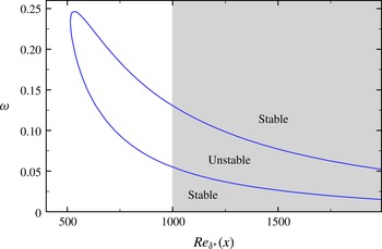
. In figure 1, the neutral curve obtained from a local spatial stability analysis performed with wall-normal profiles extracted from the base flow
 $\boldsymbol{U}_{0}$
is displayed. The unstable frequencies fall within the interval
 $0.055<{\it\omega}<0.13$
at the computational inlet and
 $0.015<{\it\omega}<0.052$
at the end of the domain.
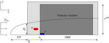
The governing equations (2.1) are solved in a computational domain
 ${\it\Omega}$
of size
 $(0,1000)\times (0,40)$
, sketched in figure 2. A Blasius profile of unit displacement thickness is prescribed at the left boundary, outflow conditions are employed at the upper and right boundaries, and a no-slip condition is imposed at the wall. The base flow
 $\boldsymbol{U}_{0}$
is imposed at the initial time for noise-driven simulations; the data used to compute the models is collected after an initial transient phase is passed. We use the spectral-element code Nek5000 (see https://nek5000.mcs.anl.gov) to perform the computations below. The computational domain is discretized using a mesh consisting of 8000 elements of spectral order 7.
Neutral curve obtained by a local spatial stability analysis; the grey area represents the extent of the computational domain.

Two different measurements are extracted from the simulations in order to compute the reduced-order model. Special emphasis is directed towards the use of data that may be readily available in an experiment, since the application of our technique to an experimental set-up is the final objective of the procedure described in this paper. We first consider a wall-friction sensor
 $s$
(see figure 2), located at
 $x_{s}=200$
and of spatial streamwise extent
 ${\rm\Delta}x=5$
, which records the wall shear-stress
 $s_{tot}$
. The fluctuating component
 $s$
may be obtained by subtracting the time-averaged value of
 $s_{tot}$
from the signal
 $s_{tot}$
. For the case of low-amplitude forcing, i.e. for linear perturbation dynamics, the time-averaged value also corresponds to the base-flow value. In addition to the wall-friction sensor
 $s$
, we also consider velocity snapshots
 $\boldsymbol{u}_{snap}$
, taken in a given domain
 ${\it\Omega}_{snap}$
of size
 $(200,900)\times (0,40)$
(see figure 2). The fluctuating components of the velocity field may again be obtained by subtracting the time-averaged snapshots from the total snapshot sequence. The wall-friction sensor was placed at the upstream edge of the velocity window. For a chosen velocity window, this set-up is optimal (not shown here) for the reconstruction of the flow field due to the highly convective behaviour of the flow. In what follows, we will consider time series of composite data comprising skin-friction measurements and velocity snapshots. The reduced-order model will be extracted from these data.
Sketch of the flow configuration. The computational domain
 ${\it\Omega}$
is of size
 $(0,1000)\times (0,40)$
, represented by the light grey box. The upstream receptivity of the boundary layer to external perturbations is modelled by the noise
 $w$
which is placed at
 $(x_{w},y_{w})=(50,0.95)$
. A sensor located at
 $(x_{s},y_{s})=(200,0)$
will identify incoming perturbations, while a velocity window of extent
 $(200,900)\times (0,40)$
(represented by the dark grey box) is used to quantify the effect of the forcing on the velocity field.

3 Dynamic mode decomposition of noise-driven amplifier flows
This section is concerned with the application of the traditional DMD technique for boundary layer flow. After a brief reminder on the underlying assumption of DMD (§ 3.1), we show that the DMD modes of boundary layer flow driven by upstream noise consist of marginally stable modes (§ 3.2), which is in contradiction with the inherent stable nature of this flow. For comparison, we then (§ 3.3) perform a DMD analysis of an impulse released by
 $w$
and show that the spectrum is qualitatively close to that obtained in global stability analyses.
3.1 Reminder on DMD
The starting point of a DMD analysis is a temporal sequence of
 $N_{snap}$
data field snapshots
 $\boldsymbol{u}(n)$
written as
 $$\begin{eqnarray}\mathsf{V}_{1}^{N_{snap}}=\{\boldsymbol{u}(1),\boldsymbol{u}(2),\ldots ,\boldsymbol{u}(N_{snap})\}.\end{eqnarray}$$
The sampling time between each snapshot
 ${\rm\Delta}t$
in the above sequence is assumed to be constant. DMD assumes that the sequence (3.1) is related by the mapping
 $$\begin{eqnarray}\boldsymbol{u}(n+1)=\unicode[STIX]{x1D63C}\boldsymbol{u}(n).\end{eqnarray}$$
Using the classical Arnoldi idea that the vectors of the sequence (3.1) sooner or later become linearly dependent, the mapping (3.2) can be expressed by
 $$\begin{eqnarray}\unicode[STIX]{x1D63C}\mathsf{V}_{1}^{N-1}=\mathsf{V}_{2}^{N}\approx \mathsf{V}_{1}^{N-1}\unicode[STIX]{x1D64E}.\end{eqnarray}$$
The eigenvalues of
 $\unicode[STIX]{x1D64E}$
(also known as the Ritz values) approximate some of the eigenvalues of
 $\unicode[STIX]{x1D63C}$
(Ruhe Reference Ruhe1984); the eigenvectors of
 $\unicode[STIX]{x1D64E}$
contain the coefficients for the reconstruction of dynamic modes expressed within the snapshot basis. The matrix
 $\unicode[STIX]{x1D64E}$
can be computed from the above equation by a least-squares approximation based on the two datasets
 $\mathsf{V}_{1}^{N-1}$
and
 $\mathsf{V}_{2}^{N}$
. We obtain
 $$\begin{eqnarray}\unicode[STIX]{x1D64E}=\unicode[STIX]{x1D64D}^{-1}\unicode[STIX]{x1D64C}^{H}\mathsf{V}_{2}^{N},\end{eqnarray}$$
where
 $\unicode[STIX]{x1D64C}$
and
 $\unicode[STIX]{x1D64D}$
stand for the QR decomposition of the dataset
 $\mathsf{V}_{1}^{N-1}$
, i.e.,
 $\unicode[STIX]{x1D64C}\unicode[STIX]{x1D64D}=\mathsf{V}_{1}^{N-1}$
. Here
 $\unicode[STIX]{x1D64C}^{H}$
denotes the Hermitian operation (complex conjugate transpose) on
 $\unicode[STIX]{x1D64C}$
. The time-discrete eigenvalues of
 $\unicode[STIX]{x1D64E}$
 $({\it\lambda}={\it\lambda}_{r}+\text{i}{\it\lambda}_{i})$
can be mapped to the time-continuous domain
 ${\it\omega}={\it\omega}_{r}+\text{i}{\it\omega}_{i}$
using the relation
 ${\it\lambda}=\text{e}^{-{\it\omega}{\rm\Delta}t}$
.
3.2 Case of driven simulation
In this section, the DMD spectrum was extracted from data obtained by performing a linearized direct numerical simulation of a boundary layer excited in
 $w$
by white noise. We used a sampling interval of
 ${\rm\Delta}t=5$
for the velocity snapshots. A dataset of length
 $N_{snap}=2000$
(
 $T=9995$
) was extracted from this simulation. This same dataset will be used in § 4 to extract the dynamic observer.
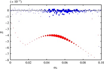
Dynamic mode spectrum in the (
 ${\it\omega}_{r},{\it\omega}_{i}$
)-plane extracted from two different datasets: white-noise-driven simulation (blue squares) and impulse response (red circles). The size of the symbols represents the relative amplitude of the velocity snapshots projected onto the dynamic modes.

The dynamic mode spectrum in the (
 ${\it\omega}_{r},{\it\omega}_{i}$
)-plane is represented in figure 3. The horizontal and vertical axes correspond, respectively, to the frequency
 ${\it\omega}_{r}$
and the growth rate
 ${\it\omega}_{i}$
. The figure is symmetric with respect to
 ${\it\omega}_{r}=0$
, and eigenvalues in the half-plane
 ${\it\omega}_{i}<0$
represent stable eigenmodes. The velocity field was projected onto the DMD modes to obtain the time-dependent dynamic mode coefficients. The relative amplitude of such coefficients is represented by the size of the symbols and indicates the importance in the dynamics of each mode.
The spectrum obtained from the driven simulation (blue squares) shows marginally stable eigenvalues. The interpretation of this result implies that the boundary layer presents self-sustained oscillations (even if the system is globally stable). This contradiction arises from DMD interpreting the unsteadiness produced by the external driving term as oscillations intrinsic to the flow. An alternative approach that separates the external driving term from the inherent stable dynamics is therefore required.
3.3 Case of impulse response
A first attempt to separate the driving term from the inherent dynamics is to perform a DMD analysis of snapshots obtained with an impulse response in
 $w$
. This amounts to performing a linearized Navier–Stokes simulation with
 $\boldsymbol{u}=\boldsymbol{F}_{w}$
as the initial condition. A DMD analysis of such snapshots should clearly identify stable global modes, which would accurately characterize the inherent dynamics of the flow.
A sampling interval
 ${\rm\Delta}t=1$
was used to extract a dataset of length
 $N_{snap}=2800$
(
 $T=2799$
). A certain amount of time is necessary for the wavepacket to reach the velocity window, since the forcing term
 $w$
is located upstream of it. This time-range, corresponding to snapshots
 $N_{snap}=0$
to
 $N_{snap}\approx 250$
(
 $T\approx 250$
), was removed from the dataset before performing the DMD analysis.
We observe in figure 3 that the eigenvalues obtained from a DMD analysis with the impulse response (marked as red circles) are stable (as expected) and display a parabolic distribution characteristic of convection–diffusion systems. These results favourably compare with the spectra obtained from global stability analyses previously reported in literature (Ehrenstein & Gallaire Reference Ehrenstein and Gallaire2005; Alizard & Robinet Reference Alizard and Robinet2007; Åkervik et al. Reference Åkervik, Ehrenstein, Gallaire and Henningson2008). The shape and amplification rate of the Tollmien–Schlichting branch roughly correspond to those reported in these articles. However, agreement is only qualitative since it was found that the details of these spectra (damping rate and separation distance between successive eigenvalues) were strongly influenced by the location and nature of the downstream boundary (Ehrenstein & Gallaire Reference Ehrenstein and Gallaire2005; Alizard & Robinet Reference Alizard and Robinet2007).
Such results clearly characterize the inherent stable dynamics of boundary layer flow. Yet in an experiment it is not possible to perform an impulse response, since the upstream driving term is unknown. We therefore need a different data-based technique to separate the inherent dynamics of the flow from the external forcing in the case of a driven flow field. This technique is presented in the next section.
4 A reduced-order dynamic observer
We first (§ 4.1) recall the technique introduced by Guzmán Iñigo et al. (Reference Guzmán Iñigo, Sipp and Schmid2014) to obtain a reduced dynamic observer, which captures the input–output dynamics from the upstream sensor
 $s$
(which stands as a proxy of the upstream driving term
 $w$
) to the velocity field. Then, in § 4.2, based on the snapshots of the driven simulation introduced in § 3.2, we compute the dominant proper orthogonal decomposition (POD) modes and build the reduced-order state-space model of the flow.
4.1 Reminder on identified dynamic observers
Considering (2.1), the evolution of small-amplitude perturbations
 $\boldsymbol{u}$
about a given base flow for the case of a noise amplifier can be represented in the time-discrete domain by
 $\boldsymbol{u}(n+1)=\unicode[STIX]{x1D63C}_{w}\boldsymbol{u}(n)+\boldsymbol{F}w(n)$
, where
 $\unicode[STIX]{x1D63C}_{w}$
denotes the linear system operator,
 $\boldsymbol{F}w(n)$
represents the driving by external perturbations and
 $n$
stands for the
 $n$
th time step. The system dynamics is entirely driven by the term
 $\boldsymbol{F}w(n)$
, which generally represents a random external noise of unknown distribution. In the present work, we propose to capture the influence of the forcing term
 $\boldsymbol{F}w(n)$
by means of a localized sensor, specifically wall-shear stress measurements
 $s(n)$
. This approach implies the loss of the receptivity information by correlating the effect of the noise at a single point with the effect on the entire domain. A dynamic observer which describes the dynamics of
 $\boldsymbol{u}_{e}(n)$
based on the input
 $s(n)$
, instead of
 $\boldsymbol{F}w(n)$
, is introduced according to
 $$\begin{eqnarray}\boldsymbol{u}_{e}(n+1)=\unicode[STIX]{x1D63C}\boldsymbol{u}_{e}(n)+\unicode[STIX]{x1D647}s(n).\end{eqnarray}$$
The matrices
 $\unicode[STIX]{x1D63C}$
and
 $\unicode[STIX]{x1D647}$
are chosen to render the temporal evolution of
 $\boldsymbol{u}_{e}$
as close as possible to the temporal evolution of
 $\boldsymbol{u}$
. We use the approach introduced by Guzmán Iñigo et al. (Reference Guzmán Iñigo, Sipp and Schmid2014), which consists of the extraction of the above matrices from time-evolving data using system-identification techniques. However, the large number of degrees of freedom contained in the snapshots
 $\boldsymbol{u}$
makes direct application of identification techniques excessively expensive. It is thus mandatory to reduce the dimensionality of the measured data. To this end, we use POD modes (Lumley Reference Lumley1967; Sirovich Reference Sirovich1987) to form a reduced basis. We process a sequence of
 $m$
velocity snapshots extracted from the simulation in the presence of the upstream noise
 $w$
. The POD then enables us to compute a ranked orthonormal basis
 $\{\unicode[STIX]{x1D731}_{i}\}_{i=1\ldots m}$
of flow fields, satisfying
 $\langle \unicode[STIX]{x1D731}_{i},\unicode[STIX]{x1D731}_{j}\rangle ={\it\delta}_{ij},\;i,j=1,2,\ldots ,m$
, which can be expressed most conveniently as a linear combination of these
 $m$
snapshots. Here, the scalar product
 $\langle \cdot \rangle$
denotes the energy-based inner product:
 $\langle \boldsymbol{u}^{1},\boldsymbol{u}^{2}\rangle =\int _{{\it\Omega}}(u^{1}u^{2}+v^{1}v^{2})\,\text{d}x\,\text{d}y$
. Any velocity field
 $\boldsymbol{V}$
from the domain
 ${\it\Omega}$
can then be projected onto the first
 $k$
POD modes according to
 $$\begin{eqnarray}y_{i}=\langle \unicode[STIX]{x1D731}_{i},\boldsymbol{V}\rangle ,\quad i=1,2,\ldots ,k,\end{eqnarray}$$
to produce the approximate flow field
 $\boldsymbol{V}^{\prime }=\sum _{i=1}^{k}\unicode[STIX]{x1D731}_{i}y_{i}$
. Properties of the POD guarantee that, for all
 $k$
, the error
 $\Vert \boldsymbol{V}-\boldsymbol{V}^{\prime }\Vert ^{2}=\langle \boldsymbol{V}-\boldsymbol{V}^{\prime },\boldsymbol{V}-\boldsymbol{V}^{\prime }\rangle$
is minimal for the set of
 $m$
measured snapshots. For the following derivations, we define the reduced output vector given by the
 $k$
POD coefficients by
 $\boldsymbol{Y}=[y_{1},y_{2},\ldots ,y_{k}]^{\text{T}}$
and denote the reduced POD basis by
 $\mathsf{U}=[\unicode[STIX]{x1D731}_{1},\unicode[STIX]{x1D731}_{2},\ldots ,\unicode[STIX]{x1D731}_{k}]$
. The velocity snapshots
 $\boldsymbol{u}$
are projected onto these modes to obtain the time-evolving POD coefficients
 $\boldsymbol{Y}(n)$
which constitute the new output of the system. The equation governing the dynamic observer (4.1) can be projected as well onto the POD basis, leading to the equation
 $$\begin{eqnarray}\boldsymbol{Y}_{e}(n+1)=\widetilde{\unicode[STIX]{x1D63C}}\boldsymbol{Y}_{e}(n)+\widetilde{\boldsymbol{L}}s(n),\end{eqnarray}$$
where
 $\widetilde{\unicode[STIX]{x1D608}}_{i,j}=\langle \unicode[STIX]{x1D731}_{i},\unicode[STIX]{x1D63C}\unicode[STIX]{x1D731}_{j}\rangle$
and
 $\widetilde{\boldsymbol{L}}_{i}=\langle \unicode[STIX]{x1D731}_{i},\unicode[STIX]{x1D647}\rangle$
. We will seek to recover and analyse the dynamics of the system by computing these reduced-order matrices from the projected data.
System identification aims at determining the system matrices such that
 $\boldsymbol{Y}_{e}(n)$
recovers the closest possible
 $\boldsymbol{Y}(n)$
from the time series of input–output data
 $\{s(n),\boldsymbol{Y}(n)\}$
, with
 $n=n_{0},\ldots ,n_{f}$
, using statistical methods. A wide range of system-identification algorithms is available. For our case, subspace identification is a particularly convenient choice since our formulation relies on a state-space formulation (see (4.3)). A detailed explanation of the algorithm is beyond the scope of this work; a comprehensive description is given in Qin (Reference Qin2006). More specifically, the N4SID-algorithm (Van Overschee & De Moor Reference Van Overschee and De Moor1994) has been used to obtain all models in this study.
Our choice of the discrete-time formulation emerges naturally when data-based methods are considered to analyse experimental situations. However, some of the concepts of dynamical-systems theory that are introduced in the subsequent sections, such as modal analysis or the frequency response, have a more direct physical interpretation and definition when a continuous-time framework is employed. The continuous formulation of the dynamic observer (4.3) reads
 $$\begin{eqnarray}\text{d}\boldsymbol{Y}_{e}/\text{d}t=\widetilde{\unicode[STIX]{x1D63C}}^{\prime }\boldsymbol{Y}_{e}(t)+\widetilde{\boldsymbol{L}}^{\prime }s(t).\end{eqnarray}$$
The time coordinate
 $t$
is related to the time index
 $n$
by
 $t=n{\rm\Delta}t$
, with
 ${\rm\Delta}t$
representing the sampling time. A relation between the matrices of (4.3) and (4.4) can be derived, resulting in
 $\widetilde{\boldsymbol{L}}=\int _{0}^{{\rm\Delta}t}\exp [\widetilde{\unicode[STIX]{x1D63C}}^{\prime }({\rm\Delta}t-{\it\tau})]\widetilde{\boldsymbol{L}}^{\prime }\;\text{d}{\it\tau}$
associated with the discrete driving term and
 $\widetilde{\unicode[STIX]{x1D63C}}=\exp (\widetilde{\unicode[STIX]{x1D63C}}^{\prime }{\rm\Delta}t)$
denoting the evolution matrix over a time interval
 ${\rm\Delta}t$
; see Antoulas (Reference Antoulas2005) for a more comprehensive description of the discrete-to-continuous time transformation.
4.2 Model
A total of
 $N_{snap}=4000$
snapshots has been extracted from the linearized simulation. These data have been split into two parts: (1) a learning dataset, used to obtain the model, and (2) a validation dataset, used to assess its performance. The learning dataset is composed of
 $N_{snap}=2000$
(
 $T=9995$
) and corresponds to the same snapshots as those used for the DMD analysis of the driven system in § 3.2. A POD basis has been computed using a total of 1500 snapshots. Guzmán Iñigo et al. (Reference Guzmán Iñigo, Sipp and Schmid2014) reported that this length was sufficient to capture the slowest time scale (frequency) of the system.
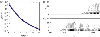
(a) First 100 POD eigenvalues
 ${\it\lambda}_{i}$
of the correlation matrix. (b) Contours of the streamwise velocity component of the first (
 $\unicode[STIX]{x1D731}_{1}$
) and tenth (
 $\unicode[STIX]{x1D731}_{10}$
) POD mode.

Figure 4(a) shows the corresponding eigenvalues of the correlation matrix, confirming a steady decay over approximately three decades in the first 30 modes (95 % of the energy is contained in the first 10 modes). Two representative POD modes,
 $\unicode[STIX]{x1D731}_{1}$
and
 $\unicode[STIX]{x1D731}_{10}$
, are displayed in figure 4(b).
Learning and validation datasets: a model is obtained using a segment of the data (with length
 $T=9995$
(grey box)); the performance of the model is then assessed in a different interval, initialized by
 $\boldsymbol{Y}_{e}=0$
at
 $t=12\,500$
. The input of the system (a) is the measurement obtained from the wall-shear sensor
 $s$
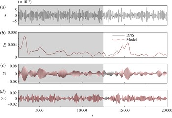
capturing the influence of external noise. (b–d) Comparison between the DNS (black) and the model prediction (red) recovered from the input for three variables: (b) the perturbation energy of the system, and (c,d) the POD coefficients
 $y_{i}$
for the first and tenth modes, respectively.

The datasets to be processed are composed of the input signal from the sensor
 $s$
and several outputs
 $y_{i}$
corresponding to the projection of the snapshots onto the basis of POD modes
 $\unicode[STIX]{x1D731}_{i}$
(figure 4). Using the N4SID algorithm, the model parameters
 $\widetilde{\unicode[STIX]{x1D63C}}$
and
 $\widetilde{\boldsymbol{L}}$
can then be determined by fitting the model output to the true, measured output, as the model is forced by the recorded input. The ability of the model to capture the dynamics of the system is then assessed on a different part of the data. For this purpose, we use the perturbation kinetic energy
 $E=\langle \boldsymbol{u}_{snap},\boldsymbol{u}_{snap}\rangle \approx \boldsymbol{Y}^{\ast }\boldsymbol{Y}$
taken from the system measurements and predicted by the model
 $\widetilde{E}(t)$
. The quality of the model can be quantified based on the fit between the temporal evolution of both magnitudes. Figure 5 shows a reduced-order model determined using
 $k=60$
POD modes and a learning dataset of length
 $T=10\,000$
. Figure 5(a) displays the measurement from the shear-stress sensor
 $s$
from which all the subsequent variables (figure 5
b–d) can be recovered using the identified model. The plotted outputs correspond to the energy (b) and the first and tenth POD coefficients (c–d). The grey box represents the data falling within the interval
 $t\in [2505,12\,500]$
used to compute the model to
 $\mathsf{FIT}_{ener}=96.87\,\%$
. The model is then initialized to
 $\boldsymbol{Y}_{e}=0$
at
 $t=12\,500$
and, after a transient period, the performance is evaluated within the interval
 $t\in [14\,505,20\,000]$
, which yields a relative match of
 $\mathsf{FIT}_{ener}=97.26\,\%$
.
The length of the transient period, estimated as
 $T\approx 1900$
, can be directly linked to the convective time scale of the disturbances. Tollmien–Schlichting waves are convected with a group velocity equal to
 $v_{g}=0.375~U_{\infty }$
(see Guzmán Iñigo et al. (Reference Guzmán Iñigo, Sipp and Schmid2014) for more details). This convective velocity defines the characteristic time
 $T_{conv}$
required by the wavepacket to cover the distance between the sensor
 $s$
and the downstream edge of the domain
 ${\it\Omega}_{snap}$
. This time
 $(T_{conv}\approx 1900)$
accurately predicts the duration of transient effects. This agreement between the time the estimator needs to propagate information and the time the system needs to convect a wavepacket confirms that the input–output behaviour of the system is properly captured by the model.
The number of POD modes considered here is rather high (
 $60$
and
 $100$
) due to the requirement for the model to accurately reconstruct the upstream measurement from the coefficients of the POD basis (Guzmán Iñigo et al.
Reference Guzmán Iñigo, Sipp and Schmid2014). This requirement is therefore linked to the observability of the sensor by the reduced basis.
5 Global modes of dynamic observer
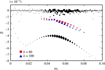
Eigenvalue spectrum in the (
 ${\it\omega}_{r},{\it\omega}_{i}$
)-plane for two different, identified reduced-order models using
 $60$
(red circles) and
 $100$
(blue triangles) POD modes. The black rectangles and diamonds represent the dynamic mode spectra depicted in figure 3.

We now turn to the computation of the eigenvalue spectrum of the identified input–output model. Considering (4.3), the temporal global spectrum of the system may be obtained by introducing an exponential time-dependence of the form
 $\boldsymbol{Y}_{e}(t)=\widehat{\boldsymbol{Y}}_{e}\text{e}^{-\text{i}{\it\omega}t}$
. We consequently obtain a generalized eigenvalue problem for
 $({\it\omega},\widehat{\boldsymbol{Y}}_{e})\in \mathbb{C}$
of the form
 $$\begin{eqnarray}\widetilde{\unicode[STIX]{x1D63C}}^{\prime }\widehat{\boldsymbol{Y}}_{e}=-\text{i}{\it\omega}\widehat{\boldsymbol{Y}}_{e}.\end{eqnarray}$$
5.1 Results
The eigenvalues
 ${\it\omega}={\it\omega}_{r}+\text{i}{\it\omega}_{i}$
are displayed in figure 6 with red (
 $k=60$
POD modes) and blue (
 $k=100$
) symbols. The spurious eigenvalues were removed by projecting the velocity snapshots onto the obtained eigenmodes, computing the mean amplitude of the time-dependent coefficients and ranking the modes as a function of this amplitude. We observe that, for the two models
 $k=60$
and
 $k=100$
, all extracted eigenvalues are stable and show similar growth rates. The damping rate and shape of the branch of identified Tollmien–Schlichting eigenvalues is again similar to those reported in global stability studies (Ehrenstein & Gallaire Reference Ehrenstein and Gallaire2005; Alizard & Robinet Reference Alizard and Robinet2007; Åkervik et al.
Reference Åkervik, Ehrenstein, Gallaire and Henningson2008).
Figure 6 also offers a comparison with the spectra obtained from the DMD analyses reported in § 3. The black squares and black diamonds respectively correspond to the results of the DMD analyses presented in figure 3 for the driven simulation and the impulse response. We observe that the eigenvalue spectra obtained with the dynamic observers are similar to the DMD spectrum obtained with the impulse response, but that the overall damping rate is different. These slight discrepancies are linked to the appreciable sensitivity of the eigenvalues in such flows. This idea will further be supported by the analysis given in the next section.
The associated global modes can be recovered using the relation
 $\widehat{\boldsymbol{V}}=\unicode[STIX]{x1D650}\widehat{\boldsymbol{Y}}_{e}$
. Based on the spectrum of the model composed of
 $60$
POD modes, the modal structures for eigenvalues with
 ${\it\omega}_{r}\approx 0.036$
,
 ${\it\omega}_{r}\approx 0.05$
,
 ${\it\omega}_{r}\approx 0.059$
and
 ${\it\omega}_{r}\approx 0.08$
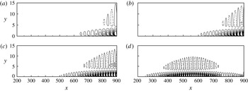
are displayed in figure 7. Contours of the real part of the streamwise velocity component
 $\widehat{\boldsymbol{V}}$
are depicted, and the perturbations are seen to be located near the wall, with the typical wavelength of the structures decreasing with increasing frequency. The amplitudes of the modes grow in the downstream direction for the three lowest frequencies, while the highest frequency displays a maximum that can be linked to the branch-II location for that particular frequency.
In the next section, we will show that the characteristics of the velocity window (size, location) in the case of a DMD analysis or in the case of global modes determined from a dynamic observer play a role similar to the characteristics of the computational domain (size, location) for explaining the sensitivity of the obtained eigenvalue spectra.
Contours of the real part of the eigenmodes associated with four of the eigenvalues depicted in figure 6 corresponding to the model based on
 $k=60$
POD modes:
 ${\it\omega}_{r}=0.036$
(a); 0.05 (b); 0.059 (c); 0.08 (d).

5.2 Sensitivity of global modes to the location of the velocity window
We will argue in this section that the overlap region of the direct and adjoint modes (the wavemaker region) should be fully contained in the velocity window in order to obtain converged, insensitive eigenvalues with a DMD technique or an identified dynamic observer. More precisely, we are interested in determining the sensitivity of a specific eigenvalue
 ${\it\lambda}$
to a change in the size of the velocity window
 ${\it\Omega}_{snap}$
. To this end, let us consider a standard eigenvalue problem of the form
 $\unicode[STIX]{x1D63C}\boldsymbol{v}={\it\lambda}\boldsymbol{v}$
and introduce a small perturbation
 ${\it\delta}\unicode[STIX]{x1D63C}$
of the operator
 $\unicode[STIX]{x1D63C}$
. The sensitivity
 ${\it\delta}{\it\lambda}$
of the eigenvalue due to the structural perturbation
 ${\it\delta}\unicode[STIX]{x1D63C}$
is given by
 $$\begin{eqnarray}{\it\delta}{\it\lambda}=\boldsymbol{w}^{H}{\it\delta}\unicode[STIX]{x1D63C}\boldsymbol{v},\end{eqnarray}$$
with
 $\unicode[STIX]{x1D63C}^{H}\boldsymbol{w}={\it\lambda}^{H}\boldsymbol{w}$
and
 $\boldsymbol{w}^{H}\boldsymbol{v}=1$
(Giannetti & Luchini Reference Giannetti and Luchini2007). If we partition the computational domain into two subdomains, we can recast the matrix
 $\unicode[STIX]{x1D63C}$
and vectors
 $\boldsymbol{v}$
and
 $\boldsymbol{w}$
according to
 $$\begin{eqnarray}\unicode[STIX]{x1D63C}=\left(\begin{array}{@{}cc@{}}\unicode[STIX]{x1D608}_{11} & \unicode[STIX]{x1D608}_{12}\\ \unicode[STIX]{x1D608}_{21} & \unicode[STIX]{x1D608}_{22}\end{array}\right),\quad \boldsymbol{v}=\left(\begin{array}{@{}c@{}}\boldsymbol{v}_{1}\\ \boldsymbol{ v}_{2}\end{array}\right),\quad \boldsymbol{w}=\left(\begin{array}{@{}c@{}}\boldsymbol{w}_{1}\\ \boldsymbol{ w}_{2}\end{array}\right),\end{eqnarray}$$
where the subindices
 $_{1}$
and
 $_{2}$
represent the elements corresponding to each subdomain. Let us perturb the operator
 $\unicode[STIX]{x1D63C}$
by
 $$\begin{eqnarray}{\it\delta}\unicode[STIX]{x1D63C}=-\!\left(\begin{array}{@{}cc@{}}\mathsf{0} & \unicode[STIX]{x1D608}_{12}\\ \unicode[STIX]{x1D608}_{21} & \unicode[STIX]{x1D608}_{22}\end{array}\right),\end{eqnarray}$$
leading to
 $$\begin{eqnarray}\unicode[STIX]{x1D63C}+{\it\delta}\unicode[STIX]{x1D63C}=\left(\begin{array}{@{}cc@{}}\unicode[STIX]{x1D608}_{11} & \mathsf{0}\\ \mathsf{ 0 } & \mathsf{0}\end{array}\right).\end{eqnarray}$$
The eigenvalue problem for this new matrix can be written as
 $\unicode[STIX]{x1D608}_{11}\boldsymbol{z}={\it\mu}\boldsymbol{z}$
. If
 ${\it\delta}\unicode[STIX]{x1D63C}$
is small, then
 $$\begin{eqnarray}{\it\mu}-{\it\lambda}={\it\delta}{\it\lambda}=\boldsymbol{w}^{H}{\it\delta}\unicode[STIX]{x1D63C}\boldsymbol{v}=(\boldsymbol{w}_{1}^{H}\unicode[STIX]{x1D608}_{12}\boldsymbol{v}_{2}+\boldsymbol{w}_{2}^{H}\unicode[STIX]{x1D608}_{21}\boldsymbol{v}_{1}+\boldsymbol{w}_{2}^{H}\unicode[STIX]{x1D608}_{22}\boldsymbol{v}_{2}).\end{eqnarray}$$
Considering that
 $\unicode[STIX]{x1D63C}$
is a local operator and that the pressure term in the linearized moment equations is weak, the terms
 $|\boldsymbol{w}_{1}^{H}\unicode[STIX]{x1D608}_{12}\boldsymbol{v}_{2}|$
and
 $|\boldsymbol{w}_{2}^{H}\unicode[STIX]{x1D608}_{21}\boldsymbol{v}_{1}|$
are small. We can, therefore, conclude that
 ${\it\mu}\approx {\it\lambda}$
if
 $|\boldsymbol{w}_{2}^{H}\unicode[STIX]{x1D608}_{22}\boldsymbol{v}_{2}|\ll 1$
. If
 $\boldsymbol{v}_{2}$
or
 $\boldsymbol{w}_{2}$
are close to zero, then
 $|\boldsymbol{w}_{2}^{H}\unicode[STIX]{x1D608}_{22}\boldsymbol{v}_{2}|\ll 1$
and
 ${\it\mu}\approx {\it\lambda}$
. This condition implies that the second subdomain must be outside of the ‘wavemaker’.
6 Frequency response of dynamic observer
A more robust alternative for studying the dynamics of noise amplifiers involves the frequency response. Assuming that the system (4.3) is forced by a harmonic input
 $s(t)=\text{e}^{\text{i}{\it\omega}t}$
, a response is sought in the form
 $\boldsymbol{Y}_{e}(t)=\overline{\boldsymbol{Y}}_{e}\text{e}^{\text{i}{\it\omega}t}$
, which leads to the expression
 $$\begin{eqnarray}\boldsymbol{R}({\it\omega})=\boldsymbol{Y}_{e}({\it\omega})/s({\it\omega})=(\text{i}{\it\omega}\unicode[STIX]{x1D644}-\widetilde{\unicode[STIX]{x1D63C}}^{\prime })^{-1}\widetilde{\boldsymbol{L}}^{\prime },\end{eqnarray}$$
where
 $\boldsymbol{R}({\it\omega})$
is defined as the frequency response and links the harmonic forcing to its associated response. The frequency response from the input
 $s$
to the first
 $k=60$
POD modes can also be computed from the full-order model. In this case, we cannot rely on an explicit matrix expression for
 $\boldsymbol{R}_{f}({\it\omega})$
. Instead, we need to apply an impulse in
 $w$
to the system, compute the Fourier transform of the responses in
 $s$
and
 $Y$
and finally apply the relation
 $\boldsymbol{R}_{f}({\it\omega})=\boldsymbol{Y}({\it\omega})/s({\it\omega})$
.
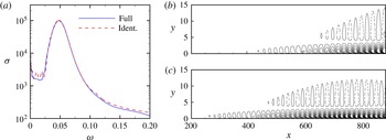
In figure 8(a) the 2-norm of the vector
 $\boldsymbol{R}({\it\omega})$
at each
 ${\it\omega}$
(which represents the square-root of the kinetic energy of the perturbation) is shown (using a blue solid line) for the full-order system and (using a red dashed line) for the reduced-order model composed of
 $k=60$
POD modes. We can report a close agreement between both models over a wide (and interesting) range of frequencies. Keeping in mind that the frequency response for the full-order system has been based on an impulse on
 $w$
, the former result implies that the bulk of the forcing noise is transmitted through the boundary layer and can be detected by a wall sensor. The response of the reduced-order model at a given frequency can be expressed in the full-order state using, once more, the relation
 $\overline{\boldsymbol{V}}({\it\omega})=\unicode[STIX]{x1D650}\overline{\boldsymbol{Y}}_{e}({\it\omega})$
. The streamwise components of the real part of the frequency response for
 ${\it\omega}\approx 0.05$
and
 ${\it\omega}\approx 0.06$
are depicted in figure 8(b). The response for both frequencies is located near the wall, and decreasing wavelengths are observed as the frequency is increased. These characteristics have also been observed in the eigenmodes computed in § 5.
(a) Transfer function from
 $s$
to the first
 $60$
POD coefficients of the full-order system (blue, solid line) and of an identified reduced-order model of size
 $k=60$
(red, dashed line). (b,c) Streamwise component of the real part of the transfer function (frequency response) from
 $s$
to the velocity field
 $V$
for two given frequencies,
 ${\it\omega}=0.05$
(b) and
 ${\it\omega}=0.06$
(c). The velocity field has been reconstructed from the identified reduced-order model depicted in (a).

The two-dimensional temporal modes exhibit a growth in amplitude as they progress downstream; this growth may be quantified by computing
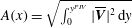 $A(x)=\sqrt{\int _{0}^{y^{PIV}}|\overline{\boldsymbol{V}}|^{2}\,\text{d}y}$
, where
 $|\cdot |$
denotes the complex modulus, and compared to the amplitude growth due to a convective instability, as predicted by a local stability analysis with
 $\boldsymbol{u}=\widehat{\boldsymbol{u}}(y)\text{e}^{\text{i}({\it\alpha}x-{\it\omega}t)}$
and
 ${\it\omega}$
and
 ${\it\alpha}$
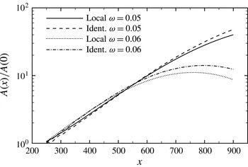
as the frequency and streamwise wavenumber of the perturbation, respectively. The comparison between the streamwise growth of the frequency response and the locally parallel flow prediction has been undertaken for the two frequencies depicted in figure 8. The corresponding
 $A(x)/A(0)$
are compared in figure 9. We notice a similar trend for the two approaches (local analyses and identified global structures), which means that an identified reduced-order model robustly captures the intrinsic dynamics of the flow. The slight disagreement between the curves can be attributed to the non-parallelism of the flow (Gaster Reference Gaster1974).
Normalized amplitude
 $A(x)/A(0)$
as a function of the streamwise distance
 $x$
for the reconstructed velocity field at the two frequencies shown in figure 8(b,c); comparison with a local stability analysis (solid and dotted lines).

7 Summary and conclusions
The extraction and analysis of the inherent dynamics of noise amplifiers from experimental data represents an important challenge due to the difficulty of separating the intrinsic (globally stable) behaviour from the surrounding noise environment that continuously drives and maintains the system.
A dynamic observer which accurately recovers full-state information from a single wall shear-stress measurement has been designed that relies on a POD basis and system identification techniques. Within the limitations of linear perturbation dynamics, the design process for the dynamic observer extracts the system matrix from a sequence of snapshots and shear-stress measurements. The spectrum of the system matrix describes a globally stable flow configuration that is sustained by selectively amplified random perturbations from the noise environment. The proposed method thus successfully separates the intrinsic, stable perturbation dynamics from the external noise excitation; previously only the combined (statistically stationary) dynamics could be described. The present approach can also be employed to extract the frequency response of the system. This type of analysis is significantly more robust than a spectral (eigenvalue) analysis and provides insight into the non-modal behaviour of the system.
Two main limitations that may be encountered in an experimental implementation of the dynamic observer are: (1) the restriction to linear dynamics, and (2) the restriction to two-dimensional configurations. In the first case, an extension of the present approach to nonlinear identification is possible, but its higher computational cost and challenging convergence characteristics make this extension a non-trivial undertaking.
The extension to three-dimensional flows involves using several sensors to capture the spanwise distribution of the incoming noise, as well as three-dimensional velocity measurements. Since three-dimensional particle image velocimetry (PIV) measurements require complex experimental set-ups that are not always feasible, an alternative solution can be obtained by measuring the velocity field of two-dimensional planes of relevant areas of the flow. In this case, the sensitivity of the eigenvalues to the extent and location of subdomains and to low-dimensional representations derived in this paper can be used to assess the quality of the experimentally obtained spectra.
Acknowledgements
The authors would like to thank J. C. Robinet for fruitful conversations, as well as J. C. Loiseau for his support with Nek-5000.