



1. Introduction
Thermally driven flows in liquid metals occur widely in geophysical and industrial systems, such as the Earth’s outer core, where they are responsible for the generation of the geomagnetic field (Stefani Reference Stefani2024). Rayleigh–Bénard convection (RBC), in which a fluid layer is heated from below and cooled from above, provides a canonical model system for studying such flows (Ahlers et al. Reference Ahlers, Grossmann and Lohse2009; Lohse & Xia Reference Lohse and Xia2010; Chilla & Schumacher Reference Chilla and Schumacher2012; Xia Reference Xia2013; Schumacher & Sreenivasan Reference Schumacher and Sreenivasan2020; Xia et al. Reference Xia, Huang, Xie and Zhang2023; Lohse & Shishkina Reference Lohse and Shishkina2024; Stefani Reference Stefani2024; Xia et al. Reference Xia, Chong, Ding and Zhang2025). Once the applied temperature difference exceeds a critical threshold, buoyancy drives the flow, whose dynamics is governed by the Rayleigh number
 $ \textit{Ra}$
, Prandtl number
 $ \textit{Pr}$
and the aspect ratio
 $\varGamma$
, which are defined as
 \begin{align} \textit{Ra} = \frac {\alpha g \Delta \textit{TH}^3}{\nu \kappa }, \quad \textit{Pr} = \frac {\nu }{\kappa }, \quad \varGamma = \frac {D}{H}. \end{align}
Here,
 $\alpha$
,
 $\nu$
and
 $\kappa$
denote the thermal expansion coefficient, the kinematic viscosity and the thermal diffusivity of the working fluid, respectively;
 $g$
is the gravitational acceleration constant;
 $\Delta T$
is the applied temperature difference between the bottom and top plates;
 $H$
is the height of the cell; and
 $D$
is the diameter of the cylindrical cell. For liquid metals, the kinematic viscosity
 $\nu$
is typically much smaller than the thermal diffusivity
 $\kappa$
, resulting in
 $ \textit{Pr}$
being much less than 1. This is in contrast to conventional fluids such as water or gases with
 $ \textit{Pr} \sim 1$
.
The heat transport in RBC is primarily accomplished through the convective motion of the fluid. It is commonly quantified by the Nusselt number
 $ \textit{Nu}$
, which is the ratio of the effective thermal conductivity of the system to the thermal conductivity of the quiescent fluid, and is given by
 \begin{align} \textit{Nu} = \frac {qH}{\lambda \Delta T} ,\end{align}
where
 $q$
is the heat flux supplied through the bottom plate and
 $\lambda$
is the thermal conductivity of the working fluid.
A prominent feature of turbulent RBC is the emergence of a large-scale circulation (LSC), often referred to as the ‘mean wind’ of turbulence (Krishnamurti & Howard Reference Krishnamurti and Howard1981; Castaing et al. Reference Castaing, Gunaratne, Heslot, Kadanoff, Libchaber, Thomae, Wu, Zaleski and Zanetti1989). The structure and dynamics of the LSC, as well as their influence on heat transport, have been extensively investigated, for reviews, see e.g. Ahlers et al. (Reference Ahlers, Grossmann and Lohse2009) and Xia et al. (Reference Xia, Huang, Xie and Zhang2023). Now, it is well established that the geometry of the convection cell, in particular, the aspect ratio
 $\varGamma$
, plays a crucial role in determining the LSC structure.
In cylindrical cells with
 $\varGamma = 1$
, the LSC takes the form of a single-roll mode (SRM), characterised by an up-flow and a down-flow near the sidewall that are approximately separated by an angle of
 $\pi$
(Qiu & Tong Reference Qiu and Tong2001). The structure and dynamics of this SRM have been extensively investigated (see e.g. Ahlers et al. Reference Ahlers, Grossmann and Lohse2009 and references therein). When the aspect ratio deviates from unity, the flow structure becomes increasingly complex (Wondrak et al. Reference Wondrak, Sieger, Mitra, Schindler, Stefani, Vogt and Eckert2023).
For
 $\varGamma \gt 1$
, the heat transport becomes nearly independent of
 $\varGamma$
already at
 $\varGamma \approx 4$
, whereas the temperature and velocity variance distributions remain affected by finite-aspect-ratio confinement up to
 $\varGamma \approx 16$
(Stevens et al. Reference Stevens, Hartmann, Verzicco and Lohse2024). Some experimental and numerical studies have revealed that the LSC can develop a three-dimensional (3-D) oscillatory mode, referred to as the jump-rope vortex (JRV), which has been observed in cylindrical and rectangular geometries using both water and liquid metal as working fluids (Vogt et al. Reference Vogt, Horn, Grannan and Aurnou2018a
; Horn et al. Reference Horn, Schmid and Aurnou2021; Akashi et al. Reference Akashi, Yanagisawa, Sakuraba, Schindler, Horn, Vogt and Eckert2022; Cheng et al. Reference Cheng, Mohammad, Wang, Keogh, Forer and Kelley2022; Li et al. Reference Li, Chen, Xu and Xi2022; Teimurazov et al. Reference Teimurazov, Singh, Su, Eckert, Shishkina and Vogt2023). Others have found that rolls are aligned in the horizontal direction within convection cells with large
 $\varGamma$
(Emran & Schumacher Reference Emran and Schumacher2015; Vogt et al. Reference Vogt, Ishimi, Yanagisawa, Tasaka, Sakuraba and Eckert2018b
; Akashi et al. Reference Akashi, Yanagisawa, Tasaka, Vogt, Murai and Eckert2019; Vogt et al. Reference Vogt, Yang, Schindler and Eckert2021; Yang et al. Reference Yang, Vogt and Eckert2021). In addition, centrifugal convection in a vertically aligned cylindrical annulus, which was first proposed and experimentally realised by Jiang et al. (Reference Jiang, Zhu, Wang, Huisman and Sun2020, Reference Jiang, Wang, Liu and Sun2022), has been studied extensively (Zhong et al. Reference Zhong, Wang and Sun2023; Yao et al. Reference Yao, Emran, Teimurazov and Shishkina2025; Ren et al. Reference Ren, Zhong, Lai and Sun2026). In this configuration, the large-scale flow typically consists of four or more pairs of convection rolls aligned parallel to the rotation axis (Wang et al. Reference Wang, Jiang, Liu, Zhu and Sun2022; Yao et al. Reference Yao, Emran, Teimurazov, Kriening, Song and Shishkina2026).
In contrast, for slender convection cells with
 $\varGamma \lt 1$
, the stability of the SRM decreases, and the flow tends to reorganise into a vertically stacked multi-roll structure (Verzicco & Camussi Reference Verzicco and Camussi2003; Xi & Xia Reference Xi and Xia2007, Reference Xi and Xia2008a
,Reference Xi and Xia
b
; Weiss & Ahlers Reference Weiss and Ahlers2011; Zwirner et al. Reference Zwirner, Tilgner and Shishkina2020; Paolillo et al. Reference Paolillo, Greco, Astarita and Cardone2021; Schindler et al. Reference Schindler, Eckert, Zürner, Schumacher and Vogt2022; Chen et al. Reference Chen, Xie, Yang and Ni2023; Wondrak et al. Reference Wondrak, Sieger, Mitra, Schindler, Stefani, Vogt and Eckert2023; Ren et al. Reference Ren, Tao, Xia and Xie2024a
,
Reference Ren, Tao, Zhang, Xia and Xieb
; Zheng et al. Reference Zheng, Chen, Zhang and Xi2025). In particular, direct numerical simulations by Verzicco & Camussi (Reference Verzicco and Camussi2003) showed that the flow undergoes a transition from the SRM to a double-roll mode (DRM) in a cylindrical cell with
 $\varGamma = 1/2$
. This coexistence of multiple flow modes has been confirmed experimentally by Xi & Xia (Reference Xi and Xia2008b
), who further showed that the difference in heat transport between the SRM and DRM is weak (
 ${\sim} 0.1\,\%$
) in water, and this result is consistent with the findings of Weiss & Ahlers (Reference Weiss and Ahlers2011). Subsequent studies have suggested that the transitions between different flow modes are related to the development of flow instabilities and coherent-structure interactions, such as elliptical instability (Zwirner et al. Reference Zwirner, Tilgner and Shishkina2020), and have been characterised using advanced measurement and analysis techniques such as time-resolved particle tracking velocimetry (PTV) measurements and proper orthogonal decomposition (Paolillo et al. Reference Paolillo, Greco, Astarita and Cardone2021).
In liquid metal convection with slender geometries, however, the situation can differ significantly due to the low-Prandtl-number nature of the flow. For example, in a cuboid cell with
 $\varGamma = 1/2$
, the LSC has been shown to transition from a twisted SRM structure to a planar SRM structure as
 $ \textit{Ra}$
increases. The heat transport associated with the twisted LSC, which follows a scaling of
 $ \textit{Nu}=0.026Ra^{0.37}$
, is approximately
 $35\,\%$
lower than that of the planar LSC at
 $ \textit{Ra}=1.2\times 10^6$
, for which the heat transport scales as
 $ \textit{Nu}=0.124Ra^{0.29}$
(Chen et al. Reference Chen, Xie, Yang and Ni2023). In addition, the collapse of the LSC has been reported in cylindrical cells with
 $\varGamma =1/2$
(Schindler et al. Reference Schindler, Eckert, Zürner, Schumacher and Vogt2022, Reference Schindler, Eckert, Zürner, Schumacher and Vogt2023). More recent measurements using contactless inductive flow tomography further revealed rapid switching between different flow modes and a tendency towards stabilisation of the SRM at higher
 $ \textit{Ra}$
(Wondrak et al. Reference Wondrak, Sieger, Mitra, Schindler, Stefani, Vogt and Eckert2023). Our recent studies have shown that strong spatial confinement facilitates the transition to fully developed turbulence (Ren et al. Reference Ren, Tao, Xia and Xie2024a
), and that switching from a SRM to a DRM within the oscillation state gives rise to hysteresis in a
 $\varGamma = 1/3$
cell (Ren et al. Reference Ren, Tao, Zhang, Xia and Xie2024b
).
Despite these advances, a systematic understanding of flow-mode transitions in liquid-metal convection remains incomplete. Existing studies have been carried out over different parameter ranges and geometries, making it difficult to establish a unified picture of how spatial confinement affects the organisation and dynamics of the LSC. In particular, most previous investigations have focused on cells with
 $\varGamma =1$
and
 $1/2$
, while the evolution of flow modes with further decreasing
 $\varGamma$
has not been systematically explored. Moreover, although it is well recognised that the flow structure is closely coupled to the global heat transport in liquid-metal convection (Verzicco & Camussi Reference Verzicco and Camussi2003; Chen et al. Reference Chen, Xie, Yang and Ni2023; Ren et al. Reference Ren, Tao, Zhang, Xia and Xie2024b
), the relation between different flow modes and their corresponding heat transport efficiency remains unclear.
In this work, we address these issues through an experimental study of liquid-metal convection in cylindrical cells with
 $\varGamma =1$
,
 $1/2$
and
 $1/3$
. By combining the multi-thermal probe technique with simultaneous heat-transport measurements, we investigate the transitions between different flow modes, their statistical properties and the role of spatial confinement in selecting the dominant mode. Particular attention is paid to the coupling between flow-mode dynamics and heat transport to provide a unified physical picture of how confinement governs the organisation of large-scale circulation in low-Prandtl-number convection. The central purpose is to determine which mode statistics are robust when
 $ \textit{Pr}$
is reduced by approximately two orders of magnitude and which features are specific to the low-
 $ \textit{Pr}$
liquid-metal convection.
The remainder of this paper is organised as follows. In § 2, we describe the experimental set-up and measurement methods. In § 3, we first identify the different flow modes and examine their general features in § 3.1. Next, we analyse their statistical properties and dependence on the aspect ratio in § 3.2, characterise representative DRM–SRM–DRM transition routes and DRM reversals in § 3.3, and investigate the structure and asymmetry of the DRM in the
 $\varGamma =1/3$
cell in § 3.4. Then, we quantify the heat transport associated with the different flow modes in § 3.5. Finally, the main findings are summarised in § 4.
2. Experimental set-up and methods
2.1. The convection cell
The experiments were carried out in three cylindrical convection cells with heights
 $H$
of 103.7, 208.1 and 311.8 mm, respectively. All three cells have the same inner diameter of
 $D=103.9$
mm. Thus, these configurations yield aspect ratios of
 $\varGamma = 1$
, 1/2 and 1/3, respectively. Apart from the height of the convection cell, the design and construction of the three cells are identical. For clarity, only the configuration of the cell with
 $\varGamma = 1$
is described here. A schematic of the experimental apparatus is shown in figure 1(
 $a$
). The entire set-up was mounted on an adjustable levelling table (A), constructed from aluminium, and levelled with an accuracy better than 0.029
 $^{\circ }$
. To reduce heat exchange between the table and the convection system, a bakelite plate (B) was placed on top of the table, providing thermal insulation beneath the circular copper bottom thermal shield (C). The bottom thermal shield, manufactured from copper, has an inner diameter of 148 mm and a height of 100 mm. A thin-film heater powered by a DC power supply (GW Instek Inc., PSW30-36) was attached to the outside of the bottom thermal shield. A PID programme controls the temperature of the shield, matching it to the temperature of the bottom plate to 0.01 K to minimise heat leakage.
(
 $a$
) Schematic diagram and (
 $b$
) photograph of the experimental set-up with aspect ratio
 $\varGamma = 1$
.

Figure 1. Long description
Panel A: A schematic diagram of an experimental setup for studying thermally driven flows in liquid metals. The setup includes an adjustable levelling table, a Bakelite plate, a bottom thermal shield, a stainless steel cylinder, a bottom plate, a Plexiglass sidewall, thermistor holders, Teflon rods, a top plate, and cooling water inlets and outlets. The components are arranged vertically with the adjustable levelling table at the bottom, supporting the Bakelite plate, which in turn supports the bottom thermal shield. The stainless steel cylinder is placed above the bottom thermal shield, surrounded by the Plexiglass sidewall. The thermistor holders are positioned within the stainless steel cylinder, and the Teflon rods are placed around the thermistor holders. The top plate is situated above the Teflon rods, and the cooling water inlets and outlets are located at the top of the setup. Panel B: A photograph of the experimental setup showing the actual apparatus with various components and wiring visible.
The bottom plate, with a thickness of 25 mm, was machined from oxygen-free copper and supported by a stainless steel ring (D). The central region of the bottom plate, corresponding to the fluid-contact region, was precisely machined and electroplated with a thin layer of nickel to prevent chemical corrosion of the copper by the liquid metal. A nickel–chromium alloy resistance heating wire (Omega Inc., NIC80) was embedded in machined grooves with a width of 2 mm and a depth of 4 mm on the underside of the bottom plate. The heating circuit was connected to a DC power supply (Ametek Inc., XG300-5), which provided a constant and stable heating power, with long-term output stability better than 99.99 %. To avoid electromagnetic effects on the liquid metal flow, the heating wire was arranged in two interlaced spiral patterns, with currents flowing in opposite directions. The wire was encased in fibreglass insulation and the total resistance of the heating wire circuit was measured to be
 $30.3\,\mathrm{\varOmega }$
.
The sidewall of the convection cell was constructed from a Plexiglass tube (F) with a wall thickness of 3 mm, an inner diameter of 103.9 mm and a height of 103.7 mm. To study the dynamics of the LSC using the multi-thermal probe technique, tiny hollow cylinders with a length of 10 mm, an outer diameter of 8 mm and an inner diameter of 2.5 mm were adhered to the sidewall as the thermistor holders (G). The thermistor holders were arranged at three distinct vertical positions corresponding to distances of
 $H/4$
,
 $H/2$
and
 $3H/4$
from the bottom plate, which are hereafter referred to as the bottom, middle and top heights of the sidewall, respectively. At each height, eight thermistor holders were uniformly distributed in the azimuthal direction around the sidewall to enable the reconstruction of the temperature profile. The sidewall was mechanically fixed between the bottom plate (E) and the top plate (I), ensuring precise alignment. Four Teflon rods (H) were used to apply tension between the two plates, thereby maintaining structural stability and ensuring reliable sealing of the convection cell.
A fluorine rubber O-ring was placed in a machined groove on the top (bottom) surface of the bottom (top) plate to ensure a reliable seal and prevent leakage of the liquid metal. The top plate, identical in diameter to the bottom plate and with a thickness of 37 mm, is made of oxygen-free copper. A double-spiral channel with a width of 6.5 mm and a depth of 22 mm is machined into the interior of the plate. The channel design ensures that adjacent flow paths carry cooling water in opposite directions, thereby enhancing thermal uniformity. The temperature of the top plate was regulated by a temperature-controlled water circulator (Julabo Inc., DD-1000F). Cooling water was supplied to the plate through the inlet and outlet (J) located at the top surface.
To minimise heat loss to the surroundings, the convection cell was wrapped with five layers of rubber foam insulation material (Huamei Inc., Class 1). In addition, all experiments were conducted inside a temperature-controlled thermostat box to further reduce the influence of ambient temperature fluctuations. The thermostat box was maintained close to the mean temperature of the top and bottom plates using a PID control programme.
2.2. The working fluid
A gallium–indium–tin (GaInSn) eutectic alloy with a melting point of
 $10.5\,^{\circ }\text{C}$
was employed as the working fluid in the present study. Throughout the experiments, the bulk temperature of the fluid, defined as
 $T_m=(T_t+T_b)/2$
, was maintained at an experimentally measured mean value of
 $35.04\pm 0.07\,^{\circ }\text{C}$
. The thermophysical properties of GaInSn, evaluated at the nominal temperature of
 $35\,^{\circ }\text{C}$
, are summarised in table 1 (Plevachuk et al. Reference Plevachuk, Sklyarchuk, Eckert, Gerbeth and Novakovic2014, Reference Plevachuk, Sklyarchuk, Eckert, Gerbeth and Novakovic2015), yielding a Prandtl number of
 $ \textit{Pr} = 0.029$
. Measurements were conducted over a range of temperature difference
 $\Delta T$
, spanning from 1.13 K to 31.74 K for the
 $\varGamma = 1$
cell, from 0.48 K to 23.69 K for the
 $\varGamma = 1/2$
cell and from 0.61 K to 19.54 K for the
 $\varGamma = 1/3$
cell. The associated
 $ \textit{Ra}$
values cover the range from
 $4.54\times 10^{5}$
to
 $1.27\times 10^{7}$
for the
 $\varGamma = 1$
cell, from
 $1.53\times 10^{6}$
to
 $7.59\times 10^{7}$
for the
 $\varGamma = 1/2$
cell and from
 $6.61\times 10^{6}$
to
 $2.11\times 10^{8}$
for the
 $\varGamma = 1/3$
cell. Particular care was taken during the filling of GaInSn into the convection cell to prevent oxidation of the liquid metal. Before filling, argon gas was injected into the convection cell for 24 h to displace residual oxygen. Subsequently, the alloy was introduced into the convection cell by gravitational feeding under an inert environment.
Physical properties of GaInSn at a temperature of 35
 $^{\circ }$
C.

Table 1. Long description
A table listing physical properties of GaInSn at 35 C. The table has five rows and two columns. The first column lists the properties: Mass density, Kinematic viscosity, Thermal conductivity, Thermal diffusivity, and Thermal expansion coefficient. The second column provides the corresponding values: 6.34 x 10^3 kg m^-3, 3.15 x 10^-7 m^2 s^-1, 24.9 W (mK)^-1, 1.08 x 10^-5 m^2 s^-1, and 1.24 x 10^-4 K^-1.
It is important to note that, under the present experimental configuration, a constant heat flux boundary condition is imposed at the bottom plate, while the top plate is maintained at a constant temperature. The thermal boundary condition at the sidewall can be characterised by the wall admittance, defined as
 $C=(D/2)\lambda /d_w\lambda _w$
, where
 $d_w$
is the sidewall thickness,
 $\lambda _w$
is the thermal conductivity of the sidewall and
 $\lambda$
is the thermal conductivity of the working fluid. In the present experimental set-up, the calculated value is
 $C=2248$
, which is much larger than 1, indicating that the sidewall can be reasonably approximated as adiabatic.
We note that the thermal boundary conditions at the fluid–plate interfaces are effective conjugate conditions rather than ideal boundary conditions, because the fluid is coupled to the heating and cooling systems through finite-thickness copper plates. To estimate the importance of finite-plate effects, we calculate the Biot number which is defined as
 $ \textit{Bi} = \textit{Nu}(\lambda /\lambda _{\textit{Cu}})(H_{\textit{Cu}}/H)$
, where
 $\lambda _{\textit{Cu}} = 401\,\mathrm{W(mK)^{-1}}$
is the thermal conductivity of copper,
 $\lambda = 24.9\,\mathrm{W(mK)^{-1}}$
is the thermal conductivity of GaInSn,
 $H$
is the cell height and
 $H_{\textit{Cu}}$
is the effective conduction length in the copper plate. Here,
 $H_{\textit{Cu}}$
is defined as the net copper thickness between the fluid-contacting surface and the nearest temperature-controlled channel or heating groove, rather than the total plate thickness. It is therefore obtained by subtracting the machined channel depth from the total plate thickness:
 $H_{\textit{Cu}}=15\,\mathrm{mm}$
for the top plate, where the cooling-water channel is machined into the copper plate, and
 $H_{\textit{Cu}}=21\,\mathrm{mm}$
for the bottom plate, where the resistance heating wire groove is machined into the plate. This gives
 $Bi = 0.021\sim 0.100$
for the top plate and
 $Bi = 0.030\sim 0.140$
for the bottom plate. These values are mostly below, or at most of the order of, 0.1, indicating that the temperature drop inside the copper plates is small compared with that across the fluid layer. Therefore, finite-plate and mixed-boundary effects may influence local plume emission, LSC orientation and the preferred roll configuration. However, because the same plates and boundary conditions were used for all aspect ratios, these effects are unlikely to be the primary cause of the observed variations in flow-mode statistics with
 $\varGamma$
.
2.3. The measurement method
The convection cell was instrumented with 37 thermistors (Omega Inc., 44031), each individually calibrated to an accuracy better than
 $0.01\,\mathrm{K}$
. The top-plate temperature
 $T_t$
was measured using four thermistors embedded in blind holes drilled laterally into the top plate (I). These thermistors were uniformly distributed in the azimuthal direction along a circle of radius
 $D/4$
. The bottom-plate temperature
 $T_b$
was determined from the average of five thermistors embedded in the bottom plate (E), including four thermistors arranged in the same manner as the top plate and one additional thermistor located at the geometric centre of the bottom plate. The vertical locations of these embedded thermistors were approximately
 $3\,\mathrm{mm}$
from the corresponding fluid–plate interfaces. To characterise the LSC, 24 thermistors were mounted on the Plexiglass sidewall (F) using the thermistor holders (G). The thermistors were arranged at three vertical positions,
 $H/4$
,
 $H/2$
and
 $3H/4$
from the bottom plate, with eight thermistors uniformly distributed in the azimuthal direction at each height. The resulting azimuthal temperature distributions were used to determine the structure and dynamics of the LSC. In addition, one thermistor was placed underneath the bottom plate (E), two thermistors were mounted on the bottom thermal shield (C), and one thermistor was placed inside the thermostat box to monitor the ambient temperature. The resistances of all thermistors were recorded using a digital multimeter (Keysight Inc., 34972A) at a sampling rate of
 $0.39\,\mathrm{Hz}$
and subsequently converted to temperatures using the calibration parameters obtained before the experiments.
The voltage
 $U$
and current
 $I$
applied to the heating wires embedded in the bottom plate were simultaneously measured, from which the applied heat flux was determined according to
 $q=4 \textit{UI}/(\pi D^2)$
. For each experimental run at a given
 $ \textit{Ra}$
, the heat flux
 $q$
was maintained constant. The values of
 $ \textit{Ra}$
and
 $ \textit{Nu}$
were calculated from the imposed heat flux
 $q$
and the measured temperature difference
 $\Delta T=T_b-T_t$
across the plates. The thermophysical properties of the working fluid were evaluated at the mean temperature
 $T_m=35\,^{\circ }\text{C}$
. Each measurement was conducted for a minimum duration of 8 h after the system had reached a steady state.
2.4. The multi-thermal probe technique
The multi-thermal probe technique has been extensively employed to investigate the dynamics of the LSC, including its orientation, strength, cessations and reversals (see e.g. Ahlers et al. Reference Ahlers, Grossmann and Lohse2009 and references therein). This method takes advantage of the characteristic structure of the LSC, which consists of ascending hot plumes and descending cold plumes. As the flow ascends (descends) along the sidewall, it carries hot (cold) fluid, thereby inducing a sinusoidal variation in the azimuthal temperature distribution near the sidewall. Consequently, by measuring the temperature along the perimeter of the sidewall, both the orientation and the strength of the LSC can be quantitatively determined via the sinusoidal-fitting (SF) method (Cioni et al. Reference Cioni, Ciliberto and Sommeria1997; Brown et al. Reference Brown, Nikolaenko and Ahlers2005; Xi & Xia Reference Xi and Xia2008b ; Weiss & Ahlers Reference Weiss and Ahlers2011; Xie et al. Reference Xie, Wei and Xia2013; Zürner et al. Reference Zürner, Schindler, Vogt, Eckert and Schumacher2019; Ren et al. Reference Ren, Tao, Zhang, Ni, Xia and Xie2022).
Examples of instantaneous temperature profiles measured at the top (blue squares), middle (black circles) and bottom (red triangles) heights of the sidewall for (
 $a$
) the SRM and (
 $b$
) the DRM, in a cell with
 $\varGamma = 1/3$
at
 $ \textit{Ra}=1.01\times 10^8$
. The solid, dashed and dash-dotted lines are fitted lines to the data using the first Fourier mode.

In the SF method, the azimuthal temperature profile at a given horizontal height is decomposed into discrete Fourier modes, as expressed by
 \begin{align} T(i, t) = T_0(t) + \sum _{n=1}^{N/2} \left[a_{n}(t)\cos \left(\frac {2n\pi }{N}i \right) + b_{n}(t)\sin \left(\frac {2n\pi }{N}i \right) \right] \quad (i=0, \ldots , N-1), \end{align}
where
 $T(i, t)$
denotes the temperature measured by the
 $i$
th thermistor at time
 $t$
;
 $T_0(t)$
represents the mean temperature obtained from all thermistors at the corresponding time
 $t$
;
 $N=8$
is the total number of thermistors uniformly distributed along the sidewall at a specific horizontal height;
 $n=1, 2, \ldots , N/2$
is the
 $n$
th Fourier mode; and
 $a_{n}(t)$
and
 $b_{n}(t)$
are the Fourier coefficients. Based on these coefficients, the instantaneous strength
 $\delta _n$
and azimuthal orientation
 $\theta _n$
of the LSC can be calculated as follows:
 \begin{align} \delta _n = \sqrt {{a_n}^2+{b_n}^2}, \qquad \theta _n = \textrm {arctan}\left (\frac {b_n}{a_n}\right )\!. \end{align}
For convenience, the azimuthal orientation
 $\theta _n$
is expressed in the range
 $(0,2\pi )$
.
Figure 2 presents representative examples of the instantaneous temperature profiles along with the corresponding sinusoidal fitting curves, obtained at the top (blue squares/solid line), middle (black circles/dashed line) and bottom (red triangles/dash-dotted line) heights of the LSC in a
 $\varGamma =1/3$
cell at
 $ \textit{Ra}=1.01\times 10^8$
. It is evident that the sinusoidal fitting curves accurately describe the experimental data, demonstrating excellent agreement. Furthermore, this method proves to be effective in distinguishing different flow modes. As shown in figure 2(
 $a$
), for the SRM, the ascending hot flow and descending cold flow are aligned across the different heights of the LSC. In contrast, in the DRM, as illustrated in figure 2(
 $b$
), the orientations of the ascending hot and descending cold flows differ by nearly
 $180^{\circ }$
between the top and bottom heights of the LSC, indicating a structural difference in the circulation pattern.
3. Results and discussion
3.1. General features of the LSC and identification of different flow modes
We first study the energy of the
 $n$
th Fourier mode
 $E_n$
and the total energy of all Fourier modes
 $E_t$
, which are defined as
 $E_n = {\delta _n}^2$
and
 $E_t = {\textstyle \sum _{n=1}^{4}} E_n$
, respectively. Figure 3 shows the ratio of the time-averaged energy of the
 $n$
th Fourier mode to the total time-averaged Fourier-mode energy,
 $\langle E_n \rangle /\langle E_t \rangle$
, as a function of
 $ \textit{Ra}$
in cells with different aspect ratios at the middle height of the sidewall. It can be seen that the first Fourier mode accounts for more than 70 % of the total Fourier-mode energy for all three aspect ratios and over the investigated
 $ \textit{Ra}$
range. In contrast, the second, third and fourth modes are much smaller. The first mode therefore captures the temperature variation along the sidewall and directly provides a convenient measure of the strength and orientation of the hot-upflow/cold-downflow structure. For this reason, the flow-mode classification and the following analysis are based on the first Fourier mode (
 $n=1$
). In the following,
 $\delta _i$
and
 $\theta _i$
denote the strength and orientation of the first Fourier mode at the top (
 $i=t$
), middle (
 $i=m$
) and bottom (
 $i=b$
) heights of the sidewall.
Ratio of the time-averaged energy of the
 $n$
th Fourier mode to the time-averaged total Fourier-mode energy,
 $\langle E_n \rangle /\langle E_t \rangle$
, as a function of
 $ \textit{Ra}$
in cells with different aspect ratios at the middle height of the sidewall. Here,
 $\langle E_n \rangle = \langle {\delta _n}^2 \rangle$
is the time-averaged energy of the
 $n$
th Fourier mode, and
 $\langle E_t \rangle = {\textstyle \sum _{n=1}^{4}} \langle E_n \rangle$
is the time-averaged total energy of all Fourier modes.

Figure 4 shows some examples of the time series of the flow strength
 $\delta _i$
(
 $i=t,m,b$
) and orientation
 $\theta _i$
(
 $i=t,m,b$
) of the LSC measured at the top (
 $i=t$
, blue solid lines), middle (
 $i=m$
, black dashed lines) and bottom (
 $i=b$
, red dash-dotted lines) heights of the sidewall in cells with different
 $\varGamma$
: (
 $a$
,
 $b$
)
 $\varGamma = 1$
,
 $ \textit{Ra} = 4.01 \times 10^6$
, (
 $c$
,
 $d$
)
 $\varGamma = 1/2$
,
 $ \textit{Ra} = 3.27 \times 10^7$
and (
 $e$
,
 $f$
)
 $\varGamma = 1/3$
,
 $ \textit{Ra} = 1.01 \times 10^8$
. It is seen that the strength
 $\delta _i$
and orientation
 $\theta _i$
of the LSC in a
 $\varGamma =1$
cell at different heights are generally aligned with each other, suggesting that the LSC is in the form of a coherent single-roll structure. In addition, they fluctuate around a preferred direction at
 $\theta \sim 240^{\circ }$
. A detailed examination of
 $\theta _i$
shown in the inset of figure 4(
 $b$
) suggests that the twisting/torsional oscillation reported in water by Funfschilling & Ahlers (Reference Funfschilling and Ahlers2004) and Brown & Ahlers (Reference Brown and Ahlers2006) is also present in liquid-metal convection. It should be noted that no cessation event, i.e. a complete stop of the LSC at three heights (Brown & Ahlers Reference Brown and Ahlers2006; Xi & Xia Reference Xi and Xia2007; Xie et al. Reference Xie, Wei and Xia2013), was observed during a measurement period of 8.2 h, which corresponds to 10 120 free-fall time units, suggesting that the LSC is very robust in the
 $\varGamma =1$
cell.
In contrast, in cells with
 $\varGamma = 1/2$
and
 $1/3$
, although the strength
 $\delta _i$
of the LSC at different heights exhibits similar temporal variation, as shown in figures 4(
 $c$
) and 4(
 $e$
), the flow strength at the mid-height of the cell shows some discrepancy with those at the top and bottom heights. It reaches zero much more frequently in the
 $\varGamma =1/3$
cell. The orientations
 $\theta _i$
of the LSC at different heights display obvious irregular fluctuations with time or show occasional large deviations among different heights, as shown in figures 4(
 $d$
) and 4(
 $f$
). These observations suggest that the flow structure and dynamics have changed qualitatively in cells with
 $\varGamma = 1/2$
and
 $1/3$
when compared with the single-roll LSC in the
 $\varGamma =1$
cell. Notably, these characteristics persist across all
 $ \textit{Ra}$
studied for a given aspect ratio of the convection cell.
Examples showing the time series of the flow strength
 $\delta _i$
and orientation
 $\theta _i$
of the LSC measured at the top (
 $i=t$
, blue solid lines), middle (
 $i=m$
, black dashed lines) and bottom (
 $i=b$
, red dash-dotted lines) heights of the sidewall in cells with (
 $a$
,
 $b$
)
 $\varGamma = 1$
,
 $ \textit{Ra} = 4.01 \times 10^6$
, (
 $c$
,
 $d$
)
 $\varGamma = 1/2$
,
 $ \textit{Ra} = 3.27 \times 10^7$
and (
 $e$
,
 $f$
)
 $\varGamma = 1/3$
,
 $ \textit{Ra} = 1.01 \times 10^8$
.

To quantitatively determine the flow structure in cells with different
 $\varGamma$
and study their
 $ \textit{Ra}$
-dependence, we follow a method proposed by Xi & Xia (Reference Xi and Xia2008b
) and Weiss & Ahlers (Reference Weiss and Ahlers2011), where the angular difference among different heights
 $| \Delta \theta |_{i,j} = 180^{\circ }-|180^{\circ }-| \theta _i-\theta _j||$
is used as a proxy for the flow mode. The flow mode is classified as being in the DRM when
 $| \Delta \theta |_{t,b} \gt 120^{\circ }$
and in the SRM when none of
 $| \Delta \theta |_{i,j}, (i \ne j=t,m,b)$
exceed
 $60^{\circ }$
. If neither SRM nor DRM is observed, the flow is classified as a transition mode (TRM). The thresholds of
 $60^\circ$
and
 $120^\circ$
are adopted following previous studies (Xi & Xia Reference Xi and Xia2008b
; Weiss & Ahlers Reference Weiss and Ahlers2011) to facilitate direct comparison. To assess the robustness of this threshold-based classification, we repeated the analysis using three paired threshold sets:
 $(50^\circ ,130^\circ )$
,
 $(60^\circ ,120^\circ )$
and
 $(70^\circ ,110^\circ )$
, corresponding to deviations of
 $\pm 16.7\,\%$
and
 $\pm 8.3\,\%$
from their respective reference values of
 $60^\circ$
and
 $120^\circ$
. We find that the relative weights and
 $1-\textit{Nu}_D/\textit{Nu}_S$
are insensitive to these threshold variations. More importantly, the identified dominant modes and the main
 $ \textit{Ra}$
-dependent trends remain unchanged. These results demonstrate that our conclusions are robust with respect to the choice of the thresholds.
Figure 5(
 $a{,}b$
) shows the time-averaged value of
 $\langle |\Delta \theta |_{t,b}\rangle$
, and its standard deviation
 $\sigma _{|\Delta \theta |_{t,b}}$
as functions of
 $ \textit{Ra}$
for cells with
 $\varGamma =1$
,
 $1/2$
and
 $1/3$
. In addition to the statistics based on the full time series, the data are conditioned on the SRM and DRM, allowing the characteristics of each flow state to be compared directly. In the
 $\varGamma =1$
cell, both
 $\langle |\Delta \theta |_{t,b}\rangle$
and
 $\sigma _{|\Delta \theta |_{t,b}}$
remain small and increase only weakly with
 $ \textit{Ra}$
, indicating a coherent single-roll LSC with nearly aligned top and bottom orientations. As
 $\varGamma$
decreases to
 $1/2$
and
 $1/3$
, the overall statistics show much larger angular differences and stronger fluctuations, suggesting an apparent loss of vertical coherence of the LSC. These results are qualitatively consistent with those of Schindler et al. (Reference Schindler, Eckert, Zürner, Schumacher and Vogt2022).
To determine whether the apparent loss of coherence originates from a genuine decorrelation within an individual flow mode or from transitions between distinct large-scale flow states, we condition the angular statistics on the SRM and DRM modes. Figure 5(
 $a$
) shows that, for the
 $\varGamma =1/2$
and
 $1/3$
cells, the SRM- and DRM-conditioned angular differences vary only weakly with
 $ \textit{Ra}$
. The overall statistics are closer to the SRM statistics in the
 $\varGamma =1/2$
cell, but closer to the DRM statistics in the
 $\varGamma =1/3$
cell, reflecting the different relative weights of the two modes. This interpretation is further supported by the relative weight analysis presented later. In addition, figure 5(
 $b$
) shows that the standard deviations within the individual SRM and DRM modes are considerably smaller than those obtained from the overall statistics. Thus, the apparent loss of coherence in the overall statistics mainly results from transitions between different flow modes rather than from a progressive loss of coherence within either the SRM or the DRM. These mode-separated statistics further highlight the dominant role of aspect ratio in selecting the preferred large-scale flow structure and its apparent coherence.
(
 $a$
) Mean value
 $\langle | \Delta \theta |_{t,b} \rangle$
and (
 $b$
) standard deviation
 $\sigma _{| \Delta \theta |_{t,b}}$
of the angular difference
 $|\Delta \theta |_{t,b}$
between the top and bottom heights as functions of
 $ \textit{Ra}$
in cells with
 $\varGamma =1$
,
 $1/2$
and
 $1/3$
for the full time series (ALL) and for the conditioned SRM and DRM modes.

Figure 5. Long description
The image contains two scatter plots labeled as Panel A and Panel B. Panel A shows the mean value of the angular difference between the top and bottom heights as a function of Ra. The x-axis represents Ra on a logarithmic scale, and the y-axis represents the mean angular difference in degrees. The data points are categorized into three groups: ALL (black squares), SRM (red circles), and DRM (blue triangles). Each group is further divided into three subsets based on different conditions: 1, 1/2, and 1/3. Panel B shows the standard deviation of the angular difference between the top and bottom heights as a function of Ra. The x-axis represents Ra on a logarithmic scale, and the y-axis represents the standard deviation in degrees. The data points are categorized similarly to Panel A. Both panels illustrate how the mean value and standard deviation of the angular difference vary with Ra in different modes.
3.2. Statistical properties of flow modes and their dependence on
 $\varGamma$

3.2.1. Relative weight of different flow modes
To quantitatively characterise the relative weights
 $w_i (i=s,d,t)$
of the different flow modes, we investigate the fractions of time the flow spends in each mode over the measurement period. The relative weights
 $w_s$
,
 $w_d$
and
 $w_t$
represent the fractions of time when the flow is in the SRM, DRM and TRM, respectively. Figure 6(
 $a$
–
 $c$
) shows
 $w_s$
(black squares),
 $w_d$
(red circles) and
 $w_t$
(blue triangles) as functions of
 $ \textit{Ra}$
in the cells with (
 $a$
)
 $\varGamma = 1$
, (
 $b$
)
 $\varGamma = 1/2$
and (
 $c$
)
 $\varGamma = 1/3$
. In the
 $\varGamma =1$
cell, as shown in figure 6(
 $a$
), one observes that
 $w_s$
is
 $100\,\%$
, while
 $w_d$
and
 $w_t$
are
 $0\,\%$
, suggesting that the SRM is the dominant flow mode and there is almost no DRM or TRM. Due to the dominating role of the SRM, the relative weights
 $w_i$
of the different flow modes are independent of
 $ \textit{Ra}$
for
 $\varGamma = 1$
. In the
 $\varGamma =1/2$
cell, as shown in figure 6(
 $b$
),
 $w_s$
is approximately 60 %, and it is larger than
 $w_d$
and
 $w_t$
, which are close to each other with a value of
 ${\sim} 20\,\%$
. Meanwhile,
 $w_s$
increases with increasing
 $ \textit{Ra}$
; in contrast,
 $w_d$
decreases with increasing
 $ \textit{Ra}$
. These observations suggest that the SRM in the
 $\varGamma = 1/2$
cell becomes more robust and coherent with increasing
 $ \textit{Ra}$
, while the DRM becomes weaker. As for the data obtained in the
 $\varGamma =1/3$
cell shown in figure 6(
 $c$
),
 $w_d$
,
 $w_t$
and
 $w_s$
show almost no variation with increasing
 $ \textit{Ra}$
and are close to 58 %, 27 % and 15 %, respectively, suggesting that the DRM is the dominant flow mode in this configuration.
Although the relative weights of the different flow modes exhibit some variation with
 $ \textit{Ra}$
, their dependence on
 $ \textit{Ra}$
remains relatively weak over the parameter range investigated. We therefore calculated the Rayleigh-number-averaged relative weights of the SRM (
 $\langle w_s \rangle$
), the DRM (
 $\langle w_d \rangle$
) and the TRM (
 $\langle w_t \rangle$
) for different
 $\varGamma$
(considering all
 $ \textit{Ra}$
). These results are listed in table 2 and plotted as functions of
 $\varGamma$
in figure 6(
 $d$
). It is seen that as
 $\varGamma$
increases,
 $\langle w_s \rangle$
increases, while both
 $\langle w_d \rangle$
and
 $\langle w_t \rangle$
decrease, implying that the SRM becomes more prevalent, while the DRM and the TRM gradually diminish with increasing
 $\varGamma$
, consistent with Wondrak et al. (Reference Wondrak, Sieger, Mitra, Schindler, Stefani, Vogt and Eckert2023). The data in figure 6(
 $d$
) suggest that in cells with
 $\varGamma =1$
and
 $\varGamma =1/2$
, the SRM is the dominant flow mode. Conversely, in the cell with
 $\varGamma =1/3$
, the DRM is the dominant flow mode.
Rayleigh-number-averaged relative weights of the SRM (
 $\langle w_s \rangle$
), DRM (
 $\langle w_d \rangle$
) and TRM (
 $\langle w_t \rangle$
) for different
 $\varGamma$
in the present liquid metal convection.

Table 2. Long description
A table with three columns and four rows, including a header row. The columns are labeled with Greek letters and symbols, and the rows are labeled with numerical values. The table presents the Rayleigh-number-averaged relative weights of the SRM, DRM, and TRM for different values. Row 1: Gamma, {w_s}, {w_d}, {w_t}. Row 2: 1, 100 percent, 0 percent, 0 percent. Row 3: 1/2, 63.6 percent, 17.5 percent, 18.9 percent. Row 4: 1/3, 14.5 percent, 58.1 percent, 27.4 percent.
Relative weights of the SRM (
 $w_s$
, black squares), the DRM (
 $w_d$
, red circles) and the TRM (
 $w_t$
, blue triangles) as a function of
 $ \textit{Ra}$
in the cells with (
 $a$
)
 $\varGamma =1$
, (
 $b$
)
 $\varGamma =1/2$
and (
 $c$
)
 $\varGamma =1/3$
. Lines are provided to guide the eye. (
 $d$
) Rayleigh-number-averaged relative weights of the SRM (
 $\langle w_s \rangle$
), the DRM (
 $\langle w_d \rangle$
) and the TRM (
 $\langle w_t \rangle$
) for different
 $\varGamma$
. The published data using water as the working fluid are obtained from Xi & Xia (Reference Xi and Xia2008b
) for
 $ \textit{Pr} = 4.9{-} 5.3$
and Weiss & Ahlers (Reference Weiss and Ahlers2011) for
 $ \textit{Pr} = 4.38$
.

Figure 6. Long description
The image contains four panels, each depicting a line graph. Panel A shows the relative weights of the SRM (black squares), the DRM (red circles), and the TRM (blue triangles) as a function of the Rayleigh number (Ra) for an aspect ratio (Γ) of 1. The x-axis represents the Rayleigh number (Ra) ranging from 10^6 to 10^7, and the y-axis represents the relative weight (w–i) in percent. The SRM dominates with values close to 100 percent, while the DRM and TRM have significantly lower values. Panel B shows the same data for an aspect ratio of 1/2. The SRM still dominates but with a decreasing trend, while the DRM and TRM show slight variations. Panel C depicts the data for an aspect ratio of 1/3, where the SRM shows a decreasing trend, and the DRM and TRM exhibit more pronounced variations. Panel D shows the Rayleigh-number-averaged relative weights of the SRM, DRM, and TRM for different aspect ratios (Γ). The x-axis represents the aspect ratio (Γ) ranging from 0.3 to 1.0, and the y-axis represents the averaged relative weight (w–i) in percent. The SRM shows a decreasing trend with increasing aspect ratio, while the DRM and TRM show varying trends. The published data are obtained from Xi & Xia (2008b) for Γ = 1/2 and Weiss & Ahlers (2011) for Γ = 1, using water as the working fluid.
We now compare our data with those reported by Xi & Xia (Reference Xi and Xia2008b
) for
 $ \textit{Pr} = 4.9{-} 5.3$
and Weiss & Ahlers (Reference Weiss and Ahlers2011) for
 $ \textit{Pr} = 4.38$
, using water as the working fluid, as shown in figure 6(
 $d$
). Despite a difference of nearly two orders of magnitude in
 $ \textit{Pr}$
, the SRM remains the dominant flow mode in both liquid-metal and water convection for
 $\varGamma =1$
and
 $1/2$
, indicating that flow-mode selection at these aspect ratios is governed primarily by geometrical confinement and depends only weakly on
 $ \textit{Pr}$
. However, in the
 $\varGamma = 1/3$
cell, the system using water as the working fluid exhibits no clearly dominant mode, whereas the DRM becomes the prevailing mode in the low-
 $ \textit{Pr}$
liquid-metal system. A possible explanation is that the DRM in the liquid-metal convection forms a stronger flow structure that is relatively resistant to background turbulent perturbations. However, the weaker flow structures in water are more readily disrupted, leading to frequent switching among modes and hence no clear modal dominance. This contrast suggests that the
 $ \textit{Pr}$
dependence of flow-mode selection may become more evident under stronger confinement, although differences in experimental boundary conditions and apparatus from the present study and those from Xi & Xia (Reference Xi and Xia2008b
) may also contribute.
3.2.2. Time-averaged strength for different flow modes
Figure 7 plots the normalised time-averaged strength
 $\langle \delta _i \rangle /\Delta T$
at the top (
 $i=t$
, blue squares), middle (
 $i=m$
, black circles) and bottom (
 $i=b$
, red triangles) heights of the sidewall as functions of
 $ \textit{Ra}$
in cells with different
 $\varGamma$
. Here, the entire time series for
 $\delta _i/\Delta T$
for a given
 $ \textit{Ra}$
were averaged for panels (
 $a$
) and (
 $b$
), and the time series for
 $\delta _i/\Delta T$
in the conditioned SRM and DRM were averaged for panels (
 $c$
) and (
 $d$
), respectively. A power-law fit to the SRM data in figure 7(
 $c$
) yields
 $\langle \delta _i \rangle /\Delta T = 9.41Ra^{-0.30}$
. The resulting fit is shown as the black solid line in figure 7(
 $c$
), and the same line is reproduced in figures 7(
 $a$
), 7(
 $b$
) and 7(
 $d$
) as a common reference for comparison. From figure 7(
 $a$
), in the
 $\varGamma =1$
cell,
 $\langle \delta _m \rangle /\Delta T$
at the middle height is slightly larger than that at the top and bottom heights, which are approximately equal to each other. It is suggested that the LSC with a tilted elliptical flow structure has the greatest temperature contrast at the middle height (Xi & Xia Reference Xi and Xia2008b
). However,
 $\langle \delta _m \rangle /\Delta T$
at the middle height is the smallest compared with that at the other heights in the
 $\varGamma =1/2$
and
 $1/3$
cells, which is consistent with the relatively large weight of the DRM in these cells. When the flow is in the DRM, the flow mixes well in the region at the middle height of the sidewall, so there are no large temperature differences in this region. In addition, despite differences in magnitude among the different flow modes and aspect ratios, the data generally exhibit an
 $ \textit{Ra}$
-dependence consistent with the effective exponent
 $-0.30$
obtained from the SRM data.
Normalised time-averaged strength
 $\langle \delta _i \rangle /\Delta T$
at the top (
 $i=t$
, blue squares), middle (
 $i=m$
, black circles) and bottom (
 $i=b$
, red triangles) heights of the sidewall as a function of
 $ \textit{Ra}$
in cells with different
 $\varGamma$
: (
 $a$
) data from all flow modes; (
 $b$
) present data together with those of Xi & Xia (Reference Xi and Xia2008b
); (
 $c$
) data in the SRM and (
 $d$
) data in the DRM. The black solid line represents a power-law fit to the SRM data in panel (
 $c$
),
 $\langle \delta _i \rangle /\Delta T = 9.41Ra^{-0.30}$
, and the same line is shown in panels (
 $a$
), (
 $b$
) and (
 $d$
) for reference. Note panels (a) and (b) share the same legend and panels (c) and (d) share the same legend.

Next, we compare these results with previous experimental results in cells with the same
 $\varGamma$
reported by Xi & Xia (Reference Xi and Xia2008b
) using water as the working fluid with
 $ \textit{Pr}=4.9{-}5.3$
, as shown in figure 7(
 $b$
). It is found that these results obtained in the
 $\varGamma =1$
and
 $\varGamma =1/3$
cells are consistent with those obtained from Xi & Xia (Reference Xi and Xia2008b
), except for the result obtained in the
 $\varGamma =1/2$
cell, in which the flow strength measured at the three heights is essentially the same in water convection. Notably, the power-law function with an effective exponent
 $-0.30$
can also describe these data, although the
 $ \textit{Pr}$
of the two datasets differ by two orders of magnitude, which indicates that
 $\langle \delta _i \rangle /\Delta T$
has a weak dependence on
 $ \textit{Pr}$
.
More insight into the normalised time-averaged strength can be obtained by separating the different flow modes, as shown in figures 7(
 $c$
) and 7(
 $d$
). From figure 7(
 $c$
), one observes that all of the data at the three heights in the SRM in cells with different
 $\varGamma$
agree well with each other and nicely collapse on the power-law curve with an effective exponent
 $-0.30$
, which indicates that
 $\langle \delta _i \rangle /\Delta T$
in the SRM in different
 $\varGamma$
cells has universal characteristics and a weak dependence on
 $\varGamma$
. However, for
 $\langle \delta _i \rangle /\Delta T$
in the DRM, as shown in figure 7(
 $d$
), in both the
 $\varGamma =1/2$
and
 $1/3$
cells, the amplitudes at the top and bottom heights are equal to each other and larger than that at the middle height. The amplitudes at the different heights in the
 $\varGamma =1/3$
cell are slightly larger than those in the
 $\varGamma = 1/2$
cell, where there is an overlap in
 $ \textit{Ra}$
, suggesting that the DRM in the
 $\varGamma=1/3$
cell may be stronger than that in the
 $\varGamma=1/2$
cell.
3.3.
Different routes of the flow mode transitions in the
$\varGamma = 1/3$
cell

Although the present results show that the flow in the
 $\varGamma = 1/3$
cell undergoes frequent transitions between the SRM and the DRM, the detailed process by which the DRM transforms into the SRM and then returns to the DRM (DRM–SRM–DRM) remains unclear. In other words, the transition routes between different flow modes have not yet been well investigated. Since a statistical characterisation of these transition routes would require a much larger number of long-duration measurements, this subsection focuses on several typical DRM–SRM–DRM transition routes rather than their statistical properties. Therefore, the examples discussed in the following should be regarded as representative phenomenological routes observed in selected events, rather than as statistically established or dominant pathways.
Route 0: representative DRM-SRM-DRM transition routes involving cessation of the flow. Panels
 $(a)$
,
 $(d)$
and
 $(g)$
show the time series of the normalised flow strength
 $\delta _i/\langle \delta _i \rangle$
, while panels
 $(b)$
,
 $(e)$
and
 $(h)$
show the corresponding orientation
 $\theta _i$
at the top (
 $i=t$
, blue squares) and bottom (
 $i=b$
, red triangles) heights of the sidewall. The green dashed horizontal line marks the threshold
 $\delta _i/\langle \delta _i \rangle = 0.15$
for flow cessation and the shaded regions denote periods during which the flow is classified as being in the SRM. Panels
 $(c)$
,
 $(f)$
and
 $(i)$
show the corresponding polar plots of
 $\delta _i/\langle \delta _i \rangle$
and
 $\theta _i$
at the top (
 $i=t$
, blue squares) and bottom (
 $i=b$
, red triangles) heights of the sidewall. In the polar plots, the green dashed circle marks the same threshold
 $\delta _i/\langle \delta _i \rangle = 0.15$
. The colour bars indicate the temporal evolution in units of
 $t/t_{\textit{ff}}$
. Panels (
 $a$
–
 $c$
), (
 $d$
–
 $f$
) and (
 $g$
–
 $i$
) correspond to the simultaneous cessation of both rolls, the cessation of the top roll and the cessation of the bottom roll, respectively.

Figure 8. Long description
Panel A: A line graph shows the time series of the normalized flow strength for Route 0a. The x-axis represents time in units of t/t–ff, and the y-axis represents the normalized flow strength. The graph includes two data series: one for the top height (blue squares) and one for the bottom height (red triangles). Panel B: Another line graph shows the corresponding orientation at the top and bottom heights. The x-axis is the same as in Panel A, and the y-axis represents the orientation in units of 2π. Panel C: A polar plot displays the normalized flow strength at the top and bottom heights. The radial axis represents the normalized flow strength, and the angular axis represents the orientation. The color bar indicates the temporal evolution in t/t–ff. Panel D: A line graph shows the time series of the normalized flow strength for Route 0b. The x-axis and y-axis are the same as in Panel A. Panel E: Another line graph shows the corresponding orientation at the top and bottom heights. The x-axis and y-axis are the same as in Panel B. Panel F: A polar plot displays the normalized flow strength at the top and bottom heights. The radial and angular axes are the same as in Panel C. Panel G: A line graph shows the time series of the normalized flow strength for Route 0c. The x-axis and y-axis are the same as in Panel A. Panel H: Another line graph shows the corresponding orientation at the top and bottom heights. The x-axis and y-axis are the same as in Panel B. Panel I: A polar plot displays the normalized flow strength at the top and bottom heights. The radial and angular axes are the same as in Panel C.
Route 1: representative DRM-SRM-DRM transition routes in which the double-roll structure returns with an azimuthal rotation direction opposite to that before the transition. Panels
 $(a)$
,
 $(d)$
and
 $(g)$
show the time series of the normalised flow strength
 $\delta _i/\langle \delta _i \rangle$
, while panels
 $(b)$
,
 $(e)$
and
 $(h)$
show the corresponding orientation
 $\theta _i$
at the top (
 $i=t$
, blue squares) and bottom (
 $i=b$
, red triangles) heights of the sidewall. The green dashed horizontal line marks the threshold
 $\delta _i/\langle \delta _i \rangle = 0.15$
for flow cessations and the shaded regions denote periods during which the flow is classified as being in the SRM. Panels
 $(c)$
,
 $(f)$
and
 $(i)$
show the corresponding polar plots of
 $\delta _i/\langle \delta _i \rangle$
and
 $\theta _i$
at the top (
 $i=t$
, blue squares) and bottom (
 $i=b$
, red triangles) heights of the sidewall. In the polar plots, the green dashed circle marks the same threshold
 $\delta _i/\langle \delta _i \rangle = 0.15$
. The colour bars indicate the temporal evolution in units of
 $t/t_{\textit{ff}}$
. Panels (
 $a$
–
 $c$
), (
 $d$
–
 $f$
) and (
 $g$
–
 $i$
) correspond to the simultaneous rotation of both rolls, the rotation of the top roll, and the rotation of the bottom roll, respectively.

Route 2: representative DRM-SRM-DRM transition routes in which the double-roll structure returns with the same azimuthal rotation direction as before the transition. Panels
 $(a)$
,
 $(d)$
and
 $(g)$
show the time series of the normalised flow strength
 $\delta _i/\langle \delta _i \rangle$
, while panels
 $(b)$
,
 $(e)$
and
 $(h)$
show the corresponding orientation
 $\theta _i$
at the top (
 $i=t$
, blue squares) and bottom (
 $i=b$
, red triangles) heights of the sidewall. The green dashed horizontal line marks the threshold
 $\delta _i/\langle \delta _i \rangle = 0.15$
for flow cessation and the shaded regions denote periods during which the flow is classified as being in the SRM. Panels
 $(c)$
,
 $(f)$
and
 $(i)$
show the corresponding polar plots of
 $\delta _i/\langle \delta _i \rangle$
and
 $\theta _i$
at the top (
 $i=t$
, blue squares) and bottom (
 $i=b$
, red triangles) heights of the sidewall. In the polar plots, the green dashed circle marks the same threshold
 $\delta _i/\langle \delta _i \rangle = 0.15$
. The colour bars indicate the temporal evolution in units of
 $t/t_{\textit{ff}}$
. Panels (
 $a$
–
 $c$
), (
 $d$
–
 $f$
) and (
 $g$
–
 $i$
) correspond to the simultaneous rotation of both rolls, the rotation of the top roll and the rotation of the bottom roll, respectively.

Figure 10. Long description
Panel A: A line graph shows the time series of the normalized flow strength for R2a. The x-axis represents time in units of t/t–ff, and the y-axis represents the normalized flow strength. The graph includes two data series: one for the top height (blue squares) and one for the bottom height (red triangles). The green dashed horizontal line marks the threshold, and the shaded regions denote periods during which the flow is classified as being in the SRM. Panel B: Another line graph shows the corresponding orientation at the top and bottom heights of the sidewall for R2a. The x-axis represents time in units of t/t–ff, and the y-axis represents the orientation in units of theta_i (2pi). Panel C: A polar plot shows the orientation and strength of the LSC at the top and bottom heights of the sidewall for R2a. The green dashed circle marks the threshold, and the color bar indicates the temporal evolution in t/t–ff. Panel D: A line graph shows the time series of the normalized flow strength for R2b. The x-axis represents time in units of t/t–ff, and the y-axis represents the normalized flow strength. The graph includes two data series: one for the top height (blue squares) and one for the bottom height (red triangles). The green dashed horizontal line marks the threshold, and the shaded regions denote periods during which the flow is classified as being in the SRM. Panel E: Another line graph shows the corresponding orientation at the top and bottom heights of the sidewall for R2b. The x-axis represents time in units of t/t–ff, and the y-axis represents the orientation in units of theta_i (2pi). Panel F: A polar plot shows the orientation and strength of the LSC at the top and bottom heights of the sidewall for R2b. The green dashed circle marks the threshold, and the color bar indicates the temporal evolution in t/t–ff. Panel G: A line graph shows the time series of the normalized flow strength for R2c. The x-axis represents time in units of t/t–ff, and the y-axis represents the normalized flow strength. The graph includes two data series: one for the top height (blue squares) and one for the bottom height (red triangles). The green dashed horizontal line marks the threshold, and the shaded regions denote periods during which the flow is classified as being in the SRM. Panel H: Another line graph shows the corresponding orientation at the top and bottom heights of the sidewall for R2c. The x-axis represents time in units of t/tff, and the y-axis represents the orientation in units of theta_i (2pi). Panel I: A polar plot shows the orientation and strength of the LSC at the top and bottom heights of the sidewall for R2c. The green dashed circle marks the threshold, and the color bar indicates the temporal evolution in t/t–ff.
Three different DRM–SRM–DRM transition routes are identified: Route 0 (R0, as shown in figure 8) is characterised by the flow mode transitions caused by the cessation of the flow; Route 1 (R1, as shown in figure 9) and Route 2 (R2, as shown in figure 10) are characterised by the flow mode transitions caused by the azimuthal rotation of the flow without cessation. The key difference between R1 and R2 lies in whether the azimuthal rotation direction of the double roll reverses across the transition. For R1, the azimuthal rotation direction of the double roll reverses before and after the flow mode transition. In contrast, for R2, the azimuthal rotation direction of the double roll remains unchanged throughout the flow mode transition process.
3.3.1. Route 0
Based on the different ways of roll cessation, R0 can be further classified into R0a (cessation of both top and bottom rolls, as shown in figure 8
 $a$
–
 $c$
), R0b (cessation of the top roll, as shown in figure 8
 $d$
–
 $f$
) and R0c (cessation of the bottom roll, as shown in figure 8
 $g$
–
 $i$
).
We first examine the transition process of R0a, as shown in figure 8(
 $a$
–
 $c$
). Here, time is normalised by the free-fall time
 $t_{\textit{ff}}=H/u_{\textit{ff}}$
, where
 $u_{\textit{ff}}=\sqrt {\alpha g \varDelta \textit{TH}}$
is the free-fall velocity. At
 $t \approx 25 t_{\textit{ff}}$
, the strengths of the top and bottom rolls begin to decrease. After approximately
 $5 t_{\textit{ff}}$
, their strengths decrease to less than 15 % of the time-averaged values, indicating the cessation of the DRM. Over the next approximately
 $5 t_{\textit{ff}}$
, the strengths of the top and bottom rolls slowly recover, eventually returning to their original levels. During this period, the flow direction of the top and bottom rolls undergoes a rapid change of approximately
 $0.5\pi$
within
 $5 t_{\textit{ff}}$
, resulting in a transition of the flow mode from the DRM to the SRM. The SRM regenerates in a direction perpendicular to the original DRM flow plane. After persisting for a period of approximately 30
 $t_{\textit{ff}}$
, the SRM rotates back to re-establish the DRM.
Next, we consider the transition processes of R0b and R0c. Figures 8(
 $d$
–
 $f$
) and 8(
 $g$
–
 $i$
) show R0b and R0c, respectively. The strength of the top (bottom) roll drops below 15 % of the average value at
 $t \approx 16 t_{\textit{ff}}$
(
 $25 t_{\textit{ff}}$
), leading to its cessation. Simultaneously, the flow direction of the top (bottom) roll changes by approximately
 $\pi$
, while the strength of the bottom (top) roll increases without altering its flow direction. After a short period, the bottom (top) roll evolves into the SRM, which persists for approximately
 $30t_{\textit{ff}}$
before rotating back to re-establish the DRM.
3.3.2. Route 1 and route 2
As previously mentioned, the key difference between the R1 and R2 routes is whether the azimuthal rotation direction after the transition is opposite to (R1) or the same as (R2) that of the initial DRM, i.e. the top and bottom rolls rotate in the opposite direction (R1) or the same direction (R2) to the initial DRM. Since the transition processes of R1 (as shown in figure 9) and R2 (as shown in figure 10) are similar, we will primarily focus on R1. Depending on which roll or rolls undergo azimuthal rotation, R1 is further classified into R1a (rotation of both top and bottom rolls, as shown in figure 9
 $a$
–
 $c$
), R1b (rotation of the top roll, as shown in figure 9
 $d$
–
 $f$
) and R1c (rotation of the bottom roll, as shown in figure 9
 $g$
–
 $i$
).
We first analyse the transition process of R1a, as shown in figure 9(
 $a$
–
 $c$
). During the period
 $0 \lesssim t/t_{\textit{ff}} \lesssim 20$
, the strength of the top and bottom rolls remains close to their own average value, while their flow directions change by approximately
 $0.5 \pi$
in opposite directions, resulting in a change in the flow mode from the DRM to the SRM. The SRM regenerates in a direction perpendicular to the original DRM flow plane and persists for approximately
 $40 t_{\textit{ff}}$
. Then, the top and bottom parts of the SRM rotate back by approximately
 $0.5 \pi$
in the reverse direction, forming the DRM. In R2a, by contrast, the top and bottom parts of the SRM continue rotating in the same direction by approximately
 $0.5 \pi$
before returning to the DRM, as shown in figure 10(
 $a$
–
 $c$
).
Next, we examine the transition processes of R1b and R1c. Figures 9(
 $d$
–
 $f$
) and 9(
 $g$
–
 $i$
) show R1b and R1c, respectively. The strength of the top (bottom) roll is weaker than that of the bottom (top) roll. Over approximately
 $20 t_{\textit{ff}}$
, the flow direction of the top (bottom) roll changes by approximately
 $\pi$
, eventually merging with the bottom (top) roll to form the SRM. After persisting for a period of approximately
 $30 t_{\textit{ff}}$
, the top (bottom) part of the SRM rotates back by approximately
 $\pi$
in the reverse direction, re-establishing the DRM. It should be noted that for R2b, as shown in figure 10(
 $d$
–
 $f$
) (R2c, as shown in figure 10
 $g$
–
 $i$
), the top (bottom) part of the SRM continues rotating in the same direction by approximately
 $\pi$
before returning to the DRM.
Probability density functions (p.d.f.s) of the orientation
 $\theta _i$
at the top (
 $i = t$
, blue squares), middle (
 $i = m$
, black circles) and bottom (
 $i = b$
, red triangles) heights of the sidewall when the flow is in the (
 $a$
) SRM and the (
 $b$
) DRM at
 $ \textit{Ra}=1.01 \times 10^8$
in the
 $\varGamma =1/3$
cell.

3.3.3. Reversal of the DRM
Reversals of the LSC, conventionally defined as a reorientation of the circulation plane by approximately
 $\pi$
, have been observed in turbulent thermal convection using water as the working fluid in cells with
 $\varGamma =1$
(Sreenivasan et al. Reference Sreenivasan, Bershadskii and Niemela2002; Brown et al. Reference Brown, Nikolaenko and Ahlers2005; Xi & Xia Reference Xi and Xia2008a
; Sugiyama et al. Reference Sugiyama, Ni, Stevens, Chan, Zhou, Xi, Sun, Grossmann, Xia and Lohse2010) and
 $\varGamma =1/2$
(Xi & Xia Reference Xi and Xia2008b
; Weiss & Ahlers Reference Weiss and Ahlers2011). However, all previous studies of flow reversals have focused specifically on the SRM. To the best of our knowledge, no reversal of the DRM has yet been reported. In this work, we find that the DRM can also reverse its flow direction. In R0c, as shown in figure 8(
 $g$
–
 $i$
), the bottom roll temporarily ceases and subsequently reforms with its circulation direction changed by approximately
 $\pi$
, leading to a reversal of the restored DRM. By contrast, in R2a, as shown in figure 10(
 $a$
–
 $c$
), the reversal proceeds through a continuous azimuthal reorientation of the flow structure, without complete cessation of either roll. This result extends the concept of LSC reversal from the commonly studied SRM to the DRM and demonstrates that reversal of the DRM can occur through either a cessation or a reorientation pathway.
3.4.
Structure and asymmetry of the DRM in the
$\varGamma = 1/3$
cell

We now focus on the internal organisation of the DRM in the strongly confined cell with
 $\varGamma = 1/3$
, where this mode is statistically dominant. Figure 11 shows the p.d.f.s of the orientation
 $\theta _i$
at the top (
 $i = t$
, blue squares), middle (
 $i = m$
, black circles) and bottom (
 $i = b$
, red triangles) heights of the sidewall when the flow is in the (
 $a$
) SRM and the (
 $b$
) DRM at
 $ \textit{Ra}=1.01 \times 10^8$
in the
 $\varGamma =1/3$
cell. In figure 11(
 $a$
), the p.d.f.s of the orientation
 $\theta _i$
measured at the different heights are close to each other and peak at
 $\theta \sim 0.2\pi$
, indicating a roughly vertically coherent LSC with a well-defined preferred orientation when the flow is in the SRM. This finding is consistent with previous studies (Xi & Xia Reference Xi and Xia2008b
; Weiss & Ahlers Reference Weiss and Ahlers2011). In contrast, when the flow is in the DRM, as shown in figure 11(
 $b$
), significant differences appear in the p.d.f.s of the orientation
 $\theta _i$
at the different heights. At the top and bottom heights, the p.d.f.s of the orientation
 $\theta _i$
exhibit peaks near
 $\theta \sim 0.2\pi$
and
 $\theta \sim 1.3\pi$
, respectively, with a difference of nearly
 $\pi$
, suggesting the presence of two vertically stacked rolls rotating in opposite directions.
At the middle height, the p.d.f. of the orientation
 $\theta _m$
in the DRM is relatively uniform across orientations, but retains a weak preference for
 $\theta \sim 0.2\pi$
, consistent with the preferred orientation at the top height. This suggests that the two vertically stacked rolls are unequal in size, with a larger roll in the upper part of the cell and a smaller one in the lower part. Notably, the preferred orientation of the SRM coincides with that of the upper roll in the DRM, suggesting that the flow structure in the upper part of the cell is more robust during flow mode transitions. This, in turn, implies an asymmetry in roll strength. This asymmetry may originate from the different thermal boundary conditions at the top and bottom plates. The top plate is maintained at a constant temperature, while the bottom plate is subjected to a constant heat flux, which may lead to different boundary-layer dynamics and plume-emission behaviours, thereby breaking the vertical symmetry of the flow.
(
 $a$
) The p.d.f. of the structure factor
 $S=| \Delta \theta |_{b,m}/( | \Delta \theta |_{b,m}+| \Delta \theta |_{t,m})$
. The solid line is a sixth-order polynomial fit to the data and is provided as a guide to the eye. (
 $b$
) Normalised conditional average of the strength
 $\langle \delta _i | S \rangle / \langle \delta _i \rangle$
at the top (
 $i = t$
, blue squares) and bottom (
 $i = b$
, red triangles) heights of the sidewall.

To quantify this asymmetry when the flow is in the DRM, following Xi & Xia (Reference Xi and Xia2008b
), we employ a structure factor
 $S=\left | \Delta \theta \right |_{b,m}/(\left | \Delta \theta \right |_{b,m}+\left | \Delta \theta \right |_{t,m})$
as a quantitative indicator. Here, DRM1 with
 $S \sim 0$
denotes a double-roll structure with a smaller upper roll and a larger lower roll, whereas DRM2 with
 $S \sim 1$
characterises a double-roll structure with a larger upper roll and a smaller lower roll. DRM3 with
 $S \sim 0.5$
represents a double-roll structure with two equal-sized rolls. First, we examine the size of the rolls. Figure 12(
 $a$
) presents the p.d.f. of the structure factor
 $S$
at
 $ \textit{Ra}=1.01 \times 10^8$
in the
 $\varGamma =1/3$
cell. This plot reveals two prominent peaks near 0 and 1, suggesting that DRM1 and DRM2 are the preferred flow structures when the flow is in the DRM in a
 $\varGamma = 1/3$
cell. This finding is broadly consistent with the results reported by Xi & Xia (Reference Xi and Xia2008b
), where asymmetric double-roll states were also observed. However, the relative preference between the two asymmetric DRM states differs. In the present liquid-metal experiment, DRM2 is more probable than DRM1, whereas the opposite preference was reported in the previous water experiment (Xi & Xia Reference Xi and Xia2008b
). This difference may reflect the combined influence of
 $ \textit{Pr}$
, experimental boundary conditions, residual cell asymmetries, and possible spontaneous symmetry breaking. The origin of the asymmetric DRM states and the mechanism controlling the relative preference between DRM1 and DRM2 at different
 $ \textit{Pr}$
therefore remain open questions.
To compare the strength of the upper and lower rolls when the flow is in the DRM1, DRM2 and DRM3, we examine the normalised conditional average of the strength
 $\langle \delta _i | S \rangle / \langle \delta _i \rangle$
at the top (
 $i = t$
, blue squares) and bottom (
 $i = b$
, red triangles) heights of the sidewall at
 $ \textit{Ra}=1.01 \times 10^8$
in the
 $\varGamma =1/3$
cell, as shown in figure 12(
 $b$
). For
 $S \sim 0$
, the value
 $\langle \delta _b | S \rangle / \langle \delta _b \rangle$
at the bottom height is larger than
 $\langle \delta _t | S \rangle / \langle \delta _t \rangle$
at the top height, indicating that the strength of the larger-lower roll is stronger than that of the smaller-upper roll in the DRM1. Conversely, near
 $S \sim 1$
,
 $\langle \delta _b | S \rangle / \langle \delta _b \rangle$
at the bottom height is smaller than
 $\langle \delta _t | S \rangle / \langle \delta _t \rangle$
at the top height, suggesting that the strength of the larger-upper roll is stronger than that of the smaller-lower roll in the DRM2. In addition, near
 $S \sim 0.5$
, the values
 $\langle \delta _i | S \rangle / \langle \delta _i \rangle$
at the top and bottom heights are close to each other, implying that the strengths of the upper and lower equal-sized rolls become comparable when the flow is in the DRM3. These results demonstrate a clear coupling between roll size and roll strength, i.e. the larger roll is associated with stronger strength, while the smaller roll is weaker.
This coupling provides a natural interpretation of the preferred orientation observed in figure 11. The preferred SRM orientation coincides with that of the upper roll in the DRM, indicating that the upper part of the circulation is dynamically more robust during mode transitions. Since DRM2, characterised by a larger and stronger upper roll and a smaller and weaker lower roll, is the most probable double-roll state, the lower roll is more susceptible to disturbance and reorganisation in the process of the flow mode transition, whereas the upper roll remains comparatively stable.
3.5. Heat transport associated with different flow modes
Previous studies using water as the working fluid have demonstrated a clear correlation between flow mode and heat transport (Xi & Xia Reference Xi and Xia2008b
; Weiss & Ahlers Reference Weiss and Ahlers2011; Xie et al. Reference Xie, Ding and Xia2018). It has been shown that the maximum difference in heat transport between DRM and SRM is approximately
 $1.7\,\%$
, occurring at
 $ \textit{Ra} = 4.76\times 10^9$
, while the differences at larger
 $ \textit{Ra}$
are smaller (Weiss & Ahlers Reference Weiss and Ahlers2011). Since heat transport in liquid metal is correlated with its internal large-scale flow, we examine the influence of flow mode on heat transport in liquid metal convection by combining the multi-thermal probe technique with simultaneous heat-transport measurements. For this purpose, following Weiss & Ahlers (Reference Weiss and Ahlers2011), we construct binary state functions
 $F$
from the time series of the identified flow modes. Specifically,
 $F_{\textit{SRM}}=1$
when the flow is in the SRM and
 $F_{\textit{SRM}}=0$
otherwise (i.e. for the DRM and TRM). Similarly,
 $F_{\textit{DRM}}=1$
when the flow is in the DRM and
 $F_{\textit{DRM}}=0$
otherwise (i.e. for the SRM and TRM).
Figure 13(
 $a$
) shows representative time series of
 $F_{\textit{SRM}}$
(blue line),
 $-F_{\textit{DRM}}$
(red line) and
 $ \textit{Nu}$
(black line) measured in a cell with
 $\varGamma =1/3$
at
 $ \textit{Ra}=1.01\times 10^8$
. For visual clarity,
 $F_{\textit{DRM}}$
is plotted with a negative sign, such that the SRM and DRM appear at
 $+1$
and
 $-1$
, respectively. This sign reversal is used only for visualisation; the original binary state function
 $F_{\textit{DRM}}$
is used in the cross-correlation analysis in the following. It can be seen qualitatively that the SRM is associated with a larger
 $ \textit{Nu}$
, whereas the DRM is associated with a smaller
 $ \textit{Nu}$
. To quantify this relationship, we calculate the cross-correlation functions between the two state functions and
 $ \textit{Nu}$
, denoted by
 $C_{F_{\textit{SRM}}, \textit{Nu}}$
and
 $C_{F_{\textit{DRM}}, \textit{Nu}}$
, respectively. The normalised cross-correlation function is defined as
 \begin{align} C_{F,\textit{Nu}}(\tau )=\frac {\left \langle \left [F(t+\tau )-\langle F\rangle \right ]\left [\textit{Nu}(t)-\langle \textit{Nu}\rangle \right ]\right \rangle }{\sigma _F \sigma _{\textit{Nu}}}, \end{align}
where
 $F$
denotes either
 $F_{\textit{SRM}}$
or
 $F_{\textit{DRM}}$
,
 $\langle \boldsymbol{\cdot }\rangle$
denotes time-averaging, and
 $\sigma _F$
and
 $\sigma _{Nu}$
are the corresponding standard deviations.
The results are shown in figure 13(
 $b$
), with the SRM represented by a blue line and the DRM by a red line. With the definition of
 $C_{F,\textit{Nu}}$
in (3.1), an extremum at a negative time lag indicates that changes in the flow mode precede the corresponding heat-transport response. The time lag is normalised by the free-fall time
 $t_{\textit{ff}}$
. Both cross-correlation functions reach their extrema at approximately
 $\tau /t_{\textit{ff}} \approx -5$
, corresponding to a positive maximum for
 $C_{F_{\textit{SRM}}, \textit{Nu}}$
and a negative minimum for
 $C_{F_{\textit{DRM}}, \textit{Nu}}$
. The thermal diffusion time between the fluid-plate interface and the embedded thermistors is estimated as
 $\tau _{\textit{Cu}} \sim d^2 / \kappa _{\textit{Cu}}$
, where
 $\kappa _{\textit{Cu}} = 1.1 \times 10^{-4}\,\mathrm{m^2s^{-1}}$
and
 $d = 3\,\mathrm{mm}$
, giving
 $\tau _{\textit{Cu}} \approx 0.08\,\mathrm{s}$
, which is much shorter than the observed delay, i.e.
 $|\tau | \approx 26.25\,\mathrm{s}$
, so that the measured plate temperature could respond rapidly to changes in the fluid temperature. Thus, the negative-lag peak is unlikely to arise from heat diffusion within the copper plate, but is instead consistent with the interpretation that the heat-transport response follows the flow-mode transition after a finite delay, rather than changing instantaneously. Furthermore,
 $C_{F_{\textit{SRM}}, \textit{Nu}}$
reaches a positive maximum at
 $\tau /t_{\textit{ff}} \approx -5$
, whereas
 $C_{F_{\textit{DRM}}, \textit{Nu}}$
reaches a negative minimum at approximately the same lag. This implies that heat transport is slightly more efficient in the SRM than in the DRM. These observations are consistent with findings reported by Weiss & Ahlers (Reference Weiss and Ahlers2011) in cells with water as the working fluid.
(
 $a$
) Representative time series of the SRM state function
 $F_{\textit{SRM}}$
(blue line), the sign-reversed DRM state function
 $-F_{\textit{DRM}}$
(red line) and
 $ \textit{Nu}$
(black line). For visual clarity,
 $F_{\textit{DRM}}$
is plotted with a negative sign, such that the SRM and DRM appear at
 $+1$
and
 $-1$
, respectively. (
 $b$
) The cross-correlation functions
 $C_{F_{\textit{SRM}}, \textit{Nu}}$
(blue line) and
 $C_{F_{\textit{DRM}}, \textit{Nu}}$
(red line). The vertical dashed line marks
 $\tau /t_{\textit{ff}}=0$
. Measurements are obtained in a cell with
 $\varGamma = 1/3$
at
 $ \textit{Ra} = 1.01 \times 10^8$
.

Normalised difference in
 $ \textit{Nu}$
between the SRM and DRM in cells with
 $\varGamma = 1/2$
(red circles) and
 $\varGamma = 1/3$
(blue triangles). The error bars denote the uncertainty of
 $1- \textit{Nu}_D/\textit{Nu}_S$
estimated from the
 $ \textit{Nu}(t)$
time series and the corresponding flow-state labels. The black squares are data from Weiss & Ahlers (Reference Weiss and Ahlers2011) in a cell with
 $\varGamma = 1/2$
(
 $ \textit{Pr} = 4.38$
). The red, blue and black solid lines represent power-law fits
 $1-\textit{Nu}_{D}/\textit{Nu}_{S} = 2.87Ra^{-0.22}$
,
 $1-\textit{Nu}_{D}/\textit{Nu}_{S} = 0.36Ra^{-0.12}$
and
 $1-\textit{Nu}_{D}/\textit{Nu}_{S} = 4.91Ra^{-0.25}$
in cells with
 $\varGamma = 1/2$
(
 $ \textit{Pr} = 0.029$
),
 $\varGamma = 1/3$
(
 $ \textit{Pr} = 0.029$
) and
 $\varGamma = 1/2$
(
 $ \textit{Pr} = 4.38$
), respectively. The red dashed line represents the extrapolation of the
 $-0.22$
scaling.

To quantify the difference in heat transport between the SRM and the DRM, figure 14 presents the normalised difference in
 $ \textit{Nu}$
,
 $1-\textit{Nu}_{D}/\textit{Nu}_{S}$
as a function of
 $ \textit{Ra}$
in cells with
 $\varGamma = 1/2$
(red circles) and
 $\varGamma = 1/3$
(blue triangles). Here,
 $ \textit{Nu}_{S}$
and
 $ \textit{Nu}_{D}$
represent heat transport conditioned on the SRM and DRM, respectively. The error bars represent the standard deviations of the corresponding estimates of
 $1-\textit{Nu}_D/\textit{Nu}_S$
and provide a quantitative measure of the uncertainty. The uncertainty is relatively larger for the
 $\varGamma =1/3$
cell, likely because the number of SRM samples is smaller when DRM is the dominant flow mode. The normalised difference in
 $ \textit{Nu}$
shows a systematic dependence on
 $ \textit{Ra}$
: it decreases with increasing
 $ \textit{Ra}$
. This suggests that the heat-transport difference between the two flow modes is larger at smaller
 $ \textit{Ra}$
. Although the magnitude of this difference is small, the positive values of
 $1-\textit{Nu}_D/\textit{Nu}_S$
indicate that the SRM is generally associated with a slightly larger
 $ \textit{Nu}$
than the DRM. Power-law fits to the data yield
 $1-\textit{Nu}_{D}/\textit{Nu}_{S} = 2.87Ra^{-0.22}$
for
 $\varGamma = 1/2$
and
 $1-\textit{Nu}_{D}/\textit{Nu}_{S} = 0.36Ra^{-0.12}$
for
 $\varGamma = 1/3$
, as indicated by the red and blue solid lines in figure 14, respectively.
We next examine the effect of
 $ \textit{Pr}$
on the difference in heat transport between the SRM and the DRM. Data (black squares) obtained from Weiss & Ahlers (Reference Weiss and Ahlers2011) in a
 $\varGamma = 1/2$
cell using water as the working fluid with
 $ \textit{Pr}=4.38$
are also presented in figure 14. Consistent with the present results, the difference in
 $ \textit{Nu}$
decreases with increasing
 $ \textit{Ra}$
and follows a power-law
 $1-\textit{Nu}_{D}/\textit{Nu}_{S} = 4.91Ra^{-0.25}$
, as shown by the black solid line. This exponent is close to the value
 $-0.22$
obtained in liquid metal convection with
 $ \textit{Pr} = 0.029$
. When the
 $-0.22$
scaling is extrapolated to the
 $ \textit{Ra}$
range covered by the water measurements (red dashed line), the predicted value of
 $1-\textit{Nu}_{D}/\textit{Nu}_{S}$
for liquid-metal convection is, on average, approximately
 $19\,\%$
higher than that for water at the same
 $ \textit{Ra}$
, with the relative difference increasing weakly with
 $ \textit{Ra}$
. This suggests that the difference in
 $ \textit{Nu}$
between different flow modes may depend weakly on
 $ \textit{Pr}$
, in contrast to its much stronger dependence on
 $ \textit{Ra}$
.
4. Conclusion
In summary, we have presented a systematic investigation of the flow mode transitions and their influence on heat transport in liquid metal convection with a Prandtl number of
 $ \textit{Pr}=0.029$
in cylindrical cells with aspect ratios
 $\varGamma = 1$
,
 $1/2$
and
 $1/3$
.
A detailed statistical analysis of the flow modes reveals that the SRM dominates in the
 $\varGamma = 1$
and
 $1/2$
cells, whereas the DRM becomes the prevailing flow mode in the
 $\varGamma = 1/3$
cell. The relative weight of the SRM increases monotonically with increasing
 $\varGamma$
, while those of the DRM and TRM exhibit a decreasing trend as
 $\varGamma$
increases. Additionally, the dimensionless time-averaged strength of the SRM LSC decreases with increasing
 $ \textit{Ra}$
, following a power law
 $\langle \delta _i \rangle /\Delta T = 9.41Ra^{-0.30}$
, and exhibits a weak dependence on
 $ \textit{Pr}$
.
In the
 $\varGamma =1/3$
cell, three representative DRM–SRM–DRM transition routes are observed. Route 0 (R0) corresponds to transitions induced by the cessation of the flow, whereas Route 1 (R1) and Route 2 (R2) occur through continuous azimuthal reorientation without cessation. In R1, the double-roll reverses its azimuthal rotation direction before and after the flow mode transition, whereas in R2, the azimuthal rotation direction remains unchanged throughout the flow mode transition. Previous studies of flow reversals have focused on the SRM. Here, we show that the DRM can also reverse through either cessation or continuous azimuthal reorientation. These findings extend the concept of flow reversal from the SRM to the DRM. The DRM2, which is characterised by an asymmetric structure with a larger and stronger upper roll and a smaller and weaker lower roll, represents the dominant DRM configuration. A strong coupling between the size and strength of the rolls is observed in the DRM, with the larger roll tending to be stronger.
The flow mode is correlated with heat transport in liquid metal convection. Specifically, the SRM is associated with slightly higher heat transport, whereas the DRM is associated with slightly lower heat transport. The difference in heat transport between the SRM and DRM progressively decreases with increasing
 $ \textit{Ra}$
, following power laws
 $1-\textit{Nu}_{D}/\textit{Nu}_{S} = 2.87Ra^{-0.22}$
for
 $\varGamma = 1/2$
and
 $1-\textit{Nu}_{D}/\textit{Nu}_{S} = 0.36Ra^{-0.12}$
for
 $\varGamma = 1/3$
. In the
 $\varGamma = 1/2$
cell, the difference in heat transport at the same
 $ \textit{Ra}$
in liquid-metal convection is found to be approximately
 $19\,\%$
higher than that in convection using water as the working fluid. This suggests that the difference in heat transport between different flow modes may depend weakly on
 $ \textit{Pr}$
, in contrast to its much stronger dependence on
 $ \textit{Ra}$
.
Large-scale flows in liquid-metal convection occur across a wide range of applications, including geophysical and astrophysical systems. The present study provides a comprehensive experimental investigation of the large-scale flow dynamics and its impact on heat transport in liquid-metal convection. The comparison with moderate-
 $ \textit{Pr}$
results shows that several confinement-controlled trends persist across a wide range of
 $ \textit{Pr}$
, including the predominance of the SRM in the
 $\varGamma =1$
and
 $1/2$
cells, the overall variation of the relative weights of different flow modes with
 $\varGamma$
, and the weak
 $ \textit{Pr}$
-dependence of the dimensionless LSC strength. By contrast, the dominance of the DRM in the
 $\varGamma =1/3$
cell, the preferred DRM2 asymmetry, and a higher heat-transport difference between the SRM and DRM highlight features specific to the present low-
 $ \textit{Pr}$
liquid metal. These findings advance the fundamental understanding of large-scale flow structures in turbulent thermal convection and offer valuable data for modelling large-scale flows in turbulent convection.
Acknowledgements
We are grateful to C. Sun for insightful discussions, comments and suggestions.
Funding
This work is supported by the National Natural Science Foundation of China (Nos. 12422209, 12595303, 12595300, 12502254), Fundamental Research Funds for the Central Universities (No. xtr042024012), the China Postdoctoral Science Foundation (No. 2025M771852), the Postdoctoral Fellowship Program of CPSF (No. GZC20251278) and the Shuimu Tsinghua Scholar Program (No. 2024SM299).
Declaration of interests
The authors report no conflict of interest.


 a
 b
 Γ=1

 ∘
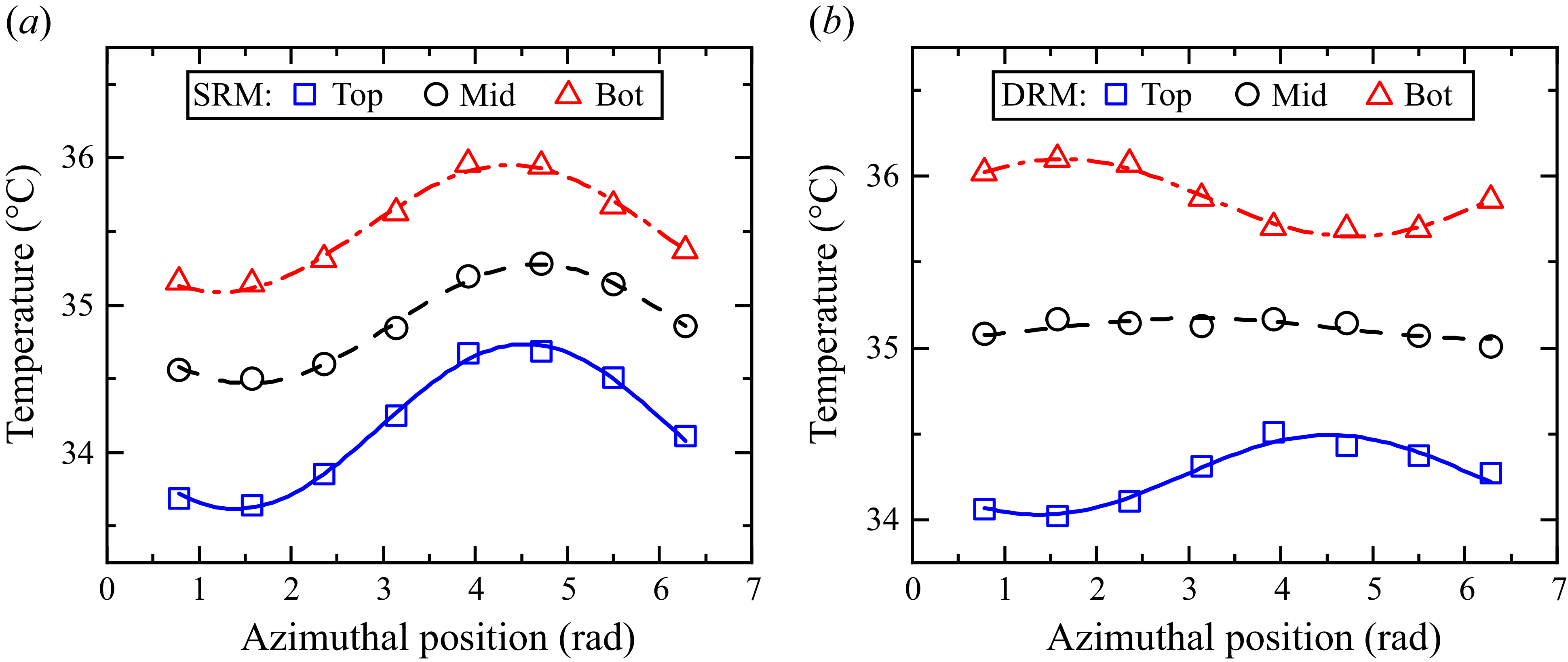
 a
 b
 Γ=1/3
 Ra=1.01×10⁸

 n
 ⟨En⟩/⟨Et⟩
 Ra
 ⟨En⟩=⟨δn2⟩
 n
 ⟨Et⟩=∑n=14⟨En⟩

 δi
 θi
 i=t
 i=m
 i=b
 a
 b
 Γ=1
 Ra=4.01×10⁶
 c
 d
 Γ=1/2
 Ra=3.27×10⁷
 e
 f
 Γ=1/3
 Ra=1.01×10⁸

 a
 ⟨|Δθ|t,b⟩
 b
 σ|Δθ|t,b
 |Δθ|t,b
 Ra
 Γ=1
 1/2
 1/3
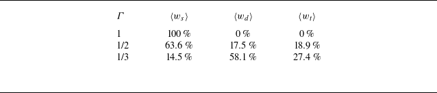
 ⟨ws⟩
 ⟨wd⟩
 ⟨wt⟩
 Γ

 ws
 wd
 wt
 Ra
 a
 Γ=1
 b
 Γ=1/2
 c
 Γ=1/3
 d
 ⟨ws⟩
 ⟨wd⟩
 ⟨wt⟩
 Γ
 Pr=4.9−5.3
 Pr=4.38

 ⟨δi⟩/ΔT
 i=t
 i=m
 i=b
 Ra
 Γ
 a
 b
 c
 d
 c
 ⟨δi⟩/ΔT=9.41Ra−0.30
 a
 b
 d

 (a)
 (d)
 (g)
 δi/⟨δi⟩
 (b)
 (e)
 (h)
 θi
 i=t
 i=b
 δi/⟨δi⟩=0.15
 (c)
 (f)
 (i)
 δi/⟨δi⟩
 θi
 i=t
 i=b
 δi/⟨δi⟩=0.15
 t/tff
 a
 c
 d
 f
 g
 i

 (a)
 (d)
 (g)
 δi/⟨δi⟩
 (b)
 (e)
 (h)
 θi
 i=t
 i=b
 δi/⟨δi⟩=0.15
 (c)
 (f)
 (i)
 δi/⟨δi⟩
 θi
 i=t
 i=b
 δi/⟨δi⟩=0.15
 t/tff
 a
 c
 d
 f
 g
 i

 (a)
 (d)
 (g)
 δi/⟨δi⟩
 (b)
 (e)
 (h)
 θi
 i=t
 i=b
 δi/⟨δi⟩=0.15
 (c)
 (f)
 (i)
 δi/⟨δi⟩
 θi
 i=t
 i=b
 δi/⟨δi⟩=0.15
 t/tff
 a
 c
 d
 f
 g
 i

 θi
 i=t
 i=m
 i=b
 a
 b
 Ra=1.01×10⁸
 Γ=1/3

 a
 S=|Δθ|b,m/(|Δθ|b,m+|Δθ|t,m)
 b
 ⟨δi|S⟩/⟨δi⟩
 i=t
 i=b

 a
 FSRM
 −FDRM
 Nu
 FDRM
 +1
 −1
 b
 CFSRM,Nu
 CFDRM,Nu
 τ/tff=0
 Γ=1/3
 Ra=1.01×10⁸

 Nu
 Γ=1/2
 Γ=1/3
 1−NuD/NuS
 Nu(t)
 Γ=1/2
 Pr=4.38
 1−NuD/NuS=2.87Ra−0.22
 1−NuD/NuS=0.36Ra−0.12
 1−NuD/NuS=4.91Ra−0.25
 Γ=1/2
 Pr=0.029
 Γ=1/3
 Pr=0.029
 Γ=1/2
 Pr=4.38
 −0.22


