1. Introduction
With the rapid development of aerospace technology, many non-cooperative on-orbit missions have emerged in the harsh space environment, such as maintenance of malfunctioning spacecraft [Reference Kalaycioglu and de Ruiter1] and active removal of space debris [Reference Rybus, Prokopczuk, Wojtunik, Aleksiejuk and Musiał2]. A feasible solution for these tasks is unmanned capture and on-orbit operation by space robots to reduce the risk associated with extravehicular activities and cost. In general, malfunctioning spacecraft and space debris are regarded as the non-cooperative tumbling target. The process of non-cooperative tumbling target capture is divided into [Reference Flores-Abad, Ma, Pham and Ulrich3]: approach, recognize, track, and capture, as shown in Figure 1. During the approach phase, the space robot flies freely to the vicinity of the non-cooperative tumbling target and then shuts down the jet engines on the base-spacecraft. During the recognition phase, the hand-eye camera at the end-effector is used to identify the motion parameters of the tumbling target. During the tracking phase, the end-effector tracks the capture point. During the capture phase, the end-effector of the space manipulator contacts the capture point and physically grasps the target. During the tracking and capture phase, in order to save fuel or avoid collisions with nearby objects, all jet engines of the base-spacecraft are turned off, so the space robot is free floating [Reference Yan, Liu, Lan, Zhang and Tu4]. This makes the dynamic coupling between the base-spacecraft and the space manipulator more significant, thereby complicating trajectory planning for the space robot.
Process for capturing non-cooperative tumbling target for space robot.

Over the past decades, many trajectory planning methods have been proposed to solve the problem of space robot capturing targets. Yan et al. [Reference Yan, Yuan, Xu, Hu and Liang5] derived the generalized relative Jacobian matrix and proposed multi-priority coordinated control based on null space mapping, realizing cooperative capture. But when the generalized Jacobian matrix is not inversible, there is the dynamic singularity of the manipulator [Reference Peng, Xu, Hu, Liang and Wu6]. The parameterization of joint angles, angular velocities, and accelerations effectively avoids dynamic singularities. Tortopidis et al. [Reference Tortopidis and Papadopoulos7] developed a trajectory parameterization technique that employs high-order polynomials as the cosine function parameters. Zhou et al. [Reference Zhou, Jin, Liu, Zhang, Liu and Liu8] proposed a reaction-null-space (RNS)-based singularity avoidance hierarchical trajectory planning method where the singular value filter decomposition method is introduced to deal with dynamic singularities. Wang et al. [Reference Wang, Luo, Fang and Yuan9] transformed the trajectory planning problem into an optimization problem using RNS and Bezier curves to parameterize the joint trajectory, and proposed a constrained differential evolution algorithm with an earlier processing strategy to solve the optimization problem. However, the above methods are suitable for capturing static non-cooperative targets, and tend to encounter challenges when capturing tumbling non-cooperative targets.
For tumbling non-cooperative target capture, scholars have also proposed many trajectory planning methods [Reference Shan, Guo and Gill10]. Xu et al. [Reference Xu, Wang, Zhang and Yang11] proposed an RNS-based adaptive control method to capture tumbling targets. Luo et al. [Reference Luo, Zong, Wang and Yuan12] proposed an optimal trajectory planning method based on the path-independent workspace to reach the capture point on the tumbling target with zero relative velocity. Xu et al. [Reference Xu, Liang, Li and Xu13] proposed a stereo-vision-based planning method to capture non-cooperative tumbling targets. Nguyen-Huynh et al. [Reference Nguyen-Huynh and Sharf14] proposed a trajectory planning method for capturing an unknown tumbling target based on the conservation of momentum, where the recursive least squares algorithm is utilized for parameter adaptation. However, these trajectory planning methods usually assume that the space target rotates with a small initial angular velocity, which limits adaptability performance.
Deep reinforcement learning (DRL), which has emerged in recent years, employs the deep artificial neural network to achieve a powerful nonlinear approximation capability, which has inspired the trajectory planning for capturing space non-cooperative tumbling targets. The agent of DRL trains a policy to maximize the cumulative reward according to the reward function of the environment, which avoids complex modeling and manual modifying parameters. DRL algorithm can be categorized into the discrete action space (DAS) algorithm and the continuous action space (CAS) algorithm. For the DAS, Xie et al. [Reference Xie, Sun, Kwan, Mu and Wu15] proposed the trajectory planning and tracking control method based on the fuzzy Q learning algorithm and time delay estimate to address model uncertainty and external disturbance. The DAS performs better for low-dimensional action space. The accuracy degrades when it is used for high-dimensional trajectory planning of the space robot. However, the curse of dimensionality arises when discretizing the continuous action space.
Fortunately, the CAS can avoid the curse of dimensionality, which is categorized into the stochastic policy gradient algorithm for continuous action space (SPGCAS) and the deterministic policy gradient algorithm for continuous action space (DPGCAS). For the SPGCAS, Wang et al. [Reference Wang, Cao, Zheng and Zhang16] proposed an end-to-end trajectory planning method based on soft actor-critic and multi-constraint optimization. Yan et al. [Reference Yan, Zhang, Liu, Wang and Liang17] employed the soft Q-learning algorithm to train a stochastic energy-based policy for motion planning of space robots. Wang et al. [Reference Wang, Zheng, Cao and Zhang18] introduced action ensembles based on Poisson distribution and proposed a multi-objective trajectory planning strategy based on proximal policy optimization. The above methods relying on stochastic policy gradients may need an extensive number of samples for gradient calculation, which consumes much time for high-dimensional action space. Furthermore, these stochastic methods generate diverse motion trajectories each time, which may not align with the precision requirements in aerospace engineering. In contrast, the DPGCAS proves more suitable for the trajectory planning of space robots. Du et al. [Reference Du, Zhou, Qi, Wang and Liu19] introduced a deep deterministic policy gradient (DDPG) method based on Pre-training skill for target capture. Hu et al. [Reference Hu, Huang, Hu, Shi and Hui20] proposed a DDPG-based constrained motion planning method, but this method is only applicable to planar manipulators and lacks in-depth analysis of reward function design. Li et al. [Reference Li, Hao, She, Li and Yu21] combined the generalized Jacobian matrix with DDPG to realize complex constraint motion planning, without accounting for the base-spacecraft disturbance. Furthermore, Wu et al. [Reference Wu, Yu, Li, He, Hua and Chen22] used DDPG to establish the online trajectory planning strategy to track dynamic targets. However, DDPG with the actor-critic method is prone to bias overestimation and error accumulation due to the temporal difference method. This leads to suboptimal policies for the trajectory planning.
Recently, some researchers have developed the twin delayed DDPG (TD3) algorithm [Reference Fujimoto, van Hoof and Meger23] as an enhancement of DDPG, where the following modifications are proposed. First, two Q value estimation function approximators are used. The update strategy of the smaller Q-value functions [Reference Bao, Zhang, Peng, Shao and Song24] is applied to avoid overestimation. Second, the delayed policy updates reduce the error accumulation and avoid blindness. Third, adding noise to the target policy during policy updates reduces the error variance between the Q-value function and the reward. The deterministic policy trained by TD3 generates deterministic actions for the initial state, enabling the practical application in space robot scenarios.
There is a strong dynamic coupling between the base-spacecraft and the manipulator of the free-floating space robot. The base-spacecraft is usually equipped with solar panels and antenna systems. The pose disturbance of the base-spacecraft seriously reduces the end-effector’s tracking accuracy, the power generation efficiency of solar panels and the communication quality with the earth station [Reference Eyiguler, Pandey, Howarth, Holley, Danskin, Hussey, Gillies and Yau25]. Therefore, when planning the trajectory for the capture mission, considering the pose disturbance is imperative. However, existing trajectory planning methods of space robots [Reference Li, Hao, She, Li and Yu21, Reference Wu, Yu, Li, He, Hua and Chen22, Reference Yan, Liu, Lan, Zhang and Tu4] based on DRL have seldom directly taken the pose disturbance of the base-spacecraft into account.
In the paper, the trajectory planning method of the space robot for non-cooperative tumbling target capture based on DRL is presented. Apart from the motion parameters of the manipulator and the generalized manipulability, the pose disturbance of the base-spacecraft is initially added to the reward function, which makes the policy have a stronger inhibitory effect on the pose disturbance of the base-spacecraft during the learning process. The remainder of the paper is organized as follows. Section 2 describes the space robot model, the kinematic model of the tumbling target, and the contact collision dynamics. Section 3 details the environment of DRL, and proposes the trajectory planning method based on TD3. Section 4 conducts numerical simulation. Section 5 summarizes the work of this paper.
2. Mathematical model
2.1. The model of the space robot
In this paper, the free-floating space robot is composed of a base-spacecraft, a space manipulator, and an end-effector, which can be modelled as an
 $n$
+1 series linkage system featuring
 $n$
active joints. The base-spacecraft is designated as link 0, and the space manipulator exhibits
 $n$
degrees of freedom (DOFs). The schematic diagram of the space robot is illustrated in Figure 2.
Schematic diagram of the space robot.

2.1.1. Kinematic model
The position vector
 $\boldsymbol{p}_{\mathrm{e}}$
of the end-effector is calculated as
 \begin{equation} \boldsymbol{p}_{\mathrm{e}}=\boldsymbol{r}_0+\boldsymbol{b}_0+\sum _{k=1}^n\left (\boldsymbol{a}_k+\boldsymbol{b}_k\right ) \end{equation}
where
 $\boldsymbol{r}_0 \in \mathbb{R}^3$
is the position vector of the base-spacecraft in the inertial coordinate system
 $O_{\mathrm{I}}-X_{\mathrm{I}} Y_{\mathrm{I}} Z_{\mathrm{I}}$
,
 $\boldsymbol{b}_0 \in \mathbb{R}^3$
is the position vector of the joint 1 in the center of mass coordinate system
 $C_0-X_0 Y_0 Z_0$
of the base-spacecraft,
 $\boldsymbol{a}_k \in \mathbb{R}^3$
is the position vector from the joint
 $J_k$
to the center of mass
 $C_k$
of the link
 $k$
, and
 $\boldsymbol{b}_k \in \mathbb{R}^3$
is the position vector from
 $C_k$
to
 $J_{k+1}$
.
According to the coupling relationship between the base-spacecraft motion and the manipulator motion of the space robot [Reference Wei, Yang, Xu and Bai34], the end-effector velocity of the manipulator is expressed as
 \begin{equation} \left [\begin{array}{c} \boldsymbol{v}_{\mathrm{e}} \\ \boldsymbol{\omega }_{\mathrm{e}} \end{array}\right ]=\boldsymbol{J}_{\mathrm{b}}\left [\begin{array}{l} \boldsymbol{v}_0 \\ \boldsymbol{\omega }_0 \end{array}\right ]+\boldsymbol{J}_{\mathrm{m}} \dot {\boldsymbol{\Theta }} \end{equation}
where
 $\boldsymbol{v}_0 \in \mathbb{R}^3$
and
 $\boldsymbol{\omega }_0 \in \mathbb{R}^3$
are the linear velocity and angular velocity of the base-spacecraft respectively,
 $\boldsymbol{J}_{\mathrm{b}} \in \mathbb{R}^{6\times 6}$
is the Jacobian matrix of the base-spacecraft,
 $\boldsymbol{J}_{\mathrm{m}} \in \mathbb{R}^{6\times n}$
is the Jacobian matrix of the manipulator, and
 $\dot {\boldsymbol{\Theta }} \in \mathbb{R}^n$
is the joint angular velocity of the manipulator.
For the purpose of simplifying the analysis, the gravitational influence on the space robot is neglected, along with the exclusion of orbital dynamics during the tracking and capture phase. Because the free-floating space robot is not affected by external forces or moments, the system’s momentum is conserved. Under the assumption of an initial linear and angular momentum of zero, the momentum conservation equation of the space robot can be derived as follows.
 \begin{equation} \left [\begin{array}{cc} M \boldsymbol{E} & M \boldsymbol{r}_{\mathrm{0 g}}^{\times \mathrm{T}} \\ M \boldsymbol{r}_{\mathrm{g}}^{\times } & \boldsymbol{I}_\omega \end{array}\right ]\left [\begin{array}{c} \boldsymbol{v}_0 \\ \boldsymbol{\omega }_0 \end{array}\right ]+\left [\begin{array}{c} \boldsymbol{J}_{\mathrm{T} \omega } \\ \boldsymbol{I}_\phi \end{array}\right ] \dot {\boldsymbol{\Theta }}=\boldsymbol{O} \end{equation}
where
 $M$
is the total mass of the space robot,
 $\boldsymbol{r}_{\mathrm{0g}}=\boldsymbol{r}_{\mathrm{g}}-\boldsymbol{r}_0 \in \mathbb{R}^3$
,
 $\boldsymbol{r}_{\mathrm{g}} \in \mathbb{R}^3$
represents the position vector of the center of mass of the space robot,
 $\boldsymbol{I}_\omega \in \mathbb{R}^{3 \times 3}$
is the inertia matrix of the base-spacecraft and the manipulator,
 $\boldsymbol{J}_{\mathrm{T} \omega } \in \mathbb{R}^{3 \times n}$
is the motion matrix of the manipulator, and
 $\boldsymbol{I}_\phi \in \mathbb{R}^{3 \times n}$
is the inertia matrix of the manipulator,
 $\boldsymbol{O}$
is the zero vector, and the symbol with
 $\times$
is the skew-symmetric matrix of the vector.
Simplifying Eq. (3) yields the coupling relationship between the base-spacecraft velocity and joint angular velocity as follows.
 \begin{equation} \begin{aligned} {\left [\begin{array}{c} \boldsymbol{v}_0 \\ \boldsymbol{\omega }_0 \end{array}\right ] } & =\left [\begin{array}{c} -\left (\boldsymbol{r}_{\mathrm{0 g}}^{\times } \boldsymbol{I}_{\mathrm{s}}^{-1} \boldsymbol{I}_{\mathrm{m}}+\frac {\boldsymbol{J}_{\mathrm{T} \omega }}{M}\right ) \\ -\boldsymbol{I}_{\mathrm{s}}^{-1} \boldsymbol{I}_{\mathrm{m}} \end{array}\right ] \dot {\boldsymbol{\Theta }} \\ & =\boldsymbol{J}_{\mathrm{bm}} \dot {\boldsymbol{\Theta }} \end{aligned} \end{equation}
where
 $\boldsymbol{J}_{\mathrm{bm}} \in \mathbb{R}^{6 \times n}$
is the coupling Jacobian matrix between the base-spacecraft and the manipulator,
 $\boldsymbol{I}_{\mathrm{s}}=\boldsymbol{I}_\omega +\boldsymbol{Mr}_{\mathrm{g}}^{\times } \boldsymbol{r}_{\mathrm{0 g}}^{\times } \in \mathbb{R}^{3 \times 3}$
, and
 $\boldsymbol{I}_{\mathrm{m}}=\boldsymbol{I}_\phi -\boldsymbol{r}_{\mathrm{g}}^{\times } \boldsymbol{J}_{\mathrm{T} \omega } \in \mathbb{R}^{3 \times n}$
.
Substituting Eq. (4) into Eq. (2), the end-effector velocity is simpified as
 \begin{equation} \begin{aligned} {\left [\begin{array}{c} \boldsymbol{v}_{\mathrm{e}} \\ \boldsymbol{\omega }_{\mathrm{e}} \end{array}\right ] } & =\left (\boldsymbol{J}_{\mathrm{b}} \boldsymbol{J}_{\mathrm{bm}}+\boldsymbol{J}_{\mathrm{m}}\right ) \dot {\boldsymbol{\Theta }} \\ & =\boldsymbol{J}_{\mathrm{g}} \dot {\boldsymbol{\Theta }} \end{aligned} \end{equation}
where
 $\boldsymbol{J}_{\mathrm{g}} \in \mathbb{R}^{6 \times n}$
is the generalized Jacobian matrix of the space robot.
2.1.2. Dynamics model
The dynamics equation of the space robot is derived employing the Lagrangian method [Reference Zhou, Luo and Wang26]
 \begin{equation} \left [\begin{array}{cc} \boldsymbol{H}_{\mathrm{b}} & \boldsymbol{H}_{\mathrm{bm}} \\ \boldsymbol{H}_{\mathrm{bm}}^{\mathrm{T}} & \boldsymbol{H}_{\mathrm{m}} \end{array}\right ]\left [\begin{array}{c} \ddot {\boldsymbol{q}}_0 \\ \ddot {\boldsymbol{\Theta }} \end{array}\right ]+\left [\begin{array}{cc} \boldsymbol{C}_{\mathrm{b}} & \boldsymbol{C}_{\mathrm{bm}} \\ \boldsymbol{C}_{\mathrm{mb}} & \boldsymbol{C}_{\mathrm{m}} \end{array}\right ]\left [\begin{array}{c} \dot {\boldsymbol{q}}_0 \\ \dot {\boldsymbol{\Theta }} \end{array}\right ]=\left [\begin{array}{c} \boldsymbol{\tau }_{\mathrm{b}} \\ \boldsymbol{\tau }_{\mathrm{m}} \end{array}\right ]+\left (\begin{array}{c} \boldsymbol{J}_{\mathrm{b}}^{\mathrm{T}} \\ \boldsymbol{J}_{\mathrm{m}}^{\mathrm{T}} \end{array}\right ) \boldsymbol{F}_{\mathrm{ci}} \end{equation}
where
 $\dot {\boldsymbol{q}}_0=\left [\boldsymbol{v}_0{ }^{\mathrm{T}}, \boldsymbol{\omega }_0{ }^{\mathrm{T}}\right ]^{\mathrm{T}} \in \mathbb{R}^6$
and
 $\ddot {\boldsymbol{q}}_0=\frac {d \dot {\boldsymbol{q}}_0}{d t}$
are the velocity and acceleration of the base-spacecraft, respectively,
 $\boldsymbol{\Theta } \in \mathbb{R}^n$
,
 $\dot {\boldsymbol{\Theta }} \in \mathbb{R}^n$
and
 $\ddot {\boldsymbol{\Theta }} \in \mathbb{R}^n$
are the joint angle, angular velocity and angular acceleration of the manipulator, respectively,
 $\boldsymbol{H}_{\mathrm{b}} \in \mathbb{R}^{6 \times 6}$
is the inertia matrix on the base-spacecraft dynamics,
 $\boldsymbol{H}_{\mathrm{m}} \in \mathbb{R}^{n \times n}$
is the inertia matrix on the manipulator dynamics,
 $\boldsymbol{H}_{\mathrm{bm}} \in \mathbb{R}^{6 \times n}$
is the dynamic coupling inertia matrix on the base-spacecraft and the manipulator,
 $\boldsymbol{C}_{\mathrm{b}} \in \mathbb{R}^{6 \times 6}$
is the nonlinear term of the base-spacecraft,
 $\boldsymbol{C}_{\mathrm{m}} \in \mathbb{R}^{n \times n}$
is the nonlinear term of the manipulator,
 $\boldsymbol{C}_{\mathrm{bm}} \in \mathbb{R}^{6 \times n}$
is the nonlinear dynamic coupling term of the base-spacecraft and the manipulator,
 $\boldsymbol{C}_{\mathrm{mb}} \in \mathbb{R}^{n \times 6}$
is the nonlinear dynamic coupling term of the manipulator and the base-spacecraft,
 $\boldsymbol{\tau }_{\mathrm{b}} \in \mathbb{R}^6$
is the external moment on the base-spacecraft,
 $\boldsymbol{\tau }_{\mathrm{m}} \in \mathbb{R}^n$
is the joint driving torque of the manipulator, and
 $\boldsymbol{F}_{\mathrm{ci}} \in \mathbb{R}^6$
is the generalized force acting on the end-effector.
Tracking phase: The space robot is free-floating, with the base-spacecraft’s thrusters inactive. So, the base-spacecraft torque
 $\boldsymbol{\tau }_{\mathrm{b}}=\boldsymbol{O}$
and the external force exerted on the end-effector
 $\boldsymbol{F}_{\mathrm{ci}}=\boldsymbol{O}$
. By substituting Eq. (5) into the upper part of Eq. (6), we get
 \begin{equation} \begin{aligned} \ddot {\boldsymbol{q}}_0 & =-\boldsymbol{H}_{\mathrm{b}}^{-1}\left (\boldsymbol{H}_{\mathrm{bm}} \ddot {\boldsymbol{\Theta }}+\boldsymbol{C}_{\mathrm{b}} \dot {\boldsymbol{q}}_0+\boldsymbol{C}_{\mathrm{bm}} \dot {\boldsymbol{\Theta }}\right ) \\ & =-\boldsymbol{H}_{\mathrm{b}}^{-1}\left (\boldsymbol{H}_{\mathrm{bm}} \ddot {\boldsymbol{\Theta }}+\boldsymbol{C}_{\mathrm{b}} \boldsymbol{J}_{\mathrm{bm}} \dot {\boldsymbol{\Theta }}+\boldsymbol{C}_{\mathrm{bm}} \dot {\boldsymbol{\Theta }}\right ) \\ & =-\boldsymbol{H}_{\mathrm{b}}^{-1} \boldsymbol{H}_{\mathrm{bm}} \ddot {\boldsymbol{\Theta }}-\boldsymbol{H}_{\mathrm{b}}^{-1}\left (\boldsymbol{C}_{\mathrm{b}} \boldsymbol{J}_{\mathrm{bm}}+\boldsymbol{C}_{\mathrm{bm}}\right ) \dot {\boldsymbol{\Theta }} \end{aligned} \end{equation}
Substituting Eq. (7) into the lower part of Eq. (6), the dynamic equation of the free-floating space robot to track the tumbling target is
 \begin{equation} \boldsymbol{H}_{\mathrm{m}}^* \ddot {\boldsymbol{\Theta }}+\boldsymbol{C}_{\mathrm{m}}^* \dot {\boldsymbol{\Theta }}=\boldsymbol{\tau }_{\mathrm{m}} \end{equation}
where the generalized inertia matrix
 \begin{equation} \boldsymbol{H}_{\mathrm{m}}^*=\boldsymbol{H}_{\mathrm{m}}-\boldsymbol{H}_{\mathrm{bm}}^{\mathrm{T}} \boldsymbol{H}_{\mathrm{b}}^{-1} \boldsymbol{H}_{\mathrm{bm}} \in \mathbb{R}^{n \times n} \end{equation}
and the generalized nonlinear term
 \begin{equation} \boldsymbol{C}_{\mathrm{m}}^*=\boldsymbol{C}_{\mathrm{mb}} \boldsymbol{J}_{\mathrm{bm}}+\boldsymbol{C}_{\mathrm{m}}-\boldsymbol{H}_{\mathrm{bm}}^{\mathrm{T}} \boldsymbol{H}_{\mathrm{b}}^{-1}\left (\boldsymbol{C}_{\mathrm{b}} \boldsymbol{J}_{\mathrm{bm}}+\boldsymbol{C}_{\mathrm{bm}}\right ) \in \mathbb{R}^{n \times n} \end{equation}
including Coriolis and centrifugal forces.
Capture phase: When the end-effector captures the tumbling target,
 $\boldsymbol{F}_{\mathrm{ci}} \neq \boldsymbol{O}$
and
 $\boldsymbol{\tau }_{\mathrm{b}}=\boldsymbol{O}$
. The dynamics equation (6) is rewritten as
 \begin{equation} \left [\begin{array}{cc} \boldsymbol{H}_{\mathrm{b}} & \boldsymbol{H}_{\mathrm{bm}} \\ \boldsymbol{H}_{\mathrm{bm}}^{\mathrm{T}} & \boldsymbol{H}_{\mathrm{m}} \end{array}\right ]\left [\begin{array}{c} \ddot {\boldsymbol{q}}_0 \\ \ddot {\boldsymbol{\Theta }} \end{array}\right ]+\left [\begin{array}{cc} \boldsymbol{C}_{\mathrm{b}} & \boldsymbol{C}_{\mathrm{bm}} \\ \boldsymbol{C}_{\mathrm{mb}} & \boldsymbol{C}_{\mathrm{m}} \end{array}\right ]\left [\begin{array}{c} \dot {\boldsymbol{q}}_0 \\ \dot {\boldsymbol{\Theta }} \end{array}\right ]=\left [\begin{array}{c} \boldsymbol{J}_{\mathrm{b}}^{\mathrm{T}} \boldsymbol{F}_{\mathrm{ci}} \\ \boldsymbol{\tau }_{\mathrm{m}}+\boldsymbol{J}_{\mathrm{m}}^{\mathrm{T}} \boldsymbol{F}_{\mathrm{ci}} \end{array}\right ] \end{equation}
Applying the above simplification method, the dynamic equation of the free-floating space robot to capture the tumbling target is obtained as
 \begin{equation} \boldsymbol{H}_{\mathrm{m}}^* \ddot {\boldsymbol{\Theta }}+\boldsymbol{C}_{\mathrm{m}}^* \dot {\boldsymbol{\Theta }}=\tilde {\boldsymbol{\tau }}_{\mathrm{m}} \end{equation}
where
 $\tilde {\boldsymbol{\tau }}_{\mathrm{m}}=\boldsymbol{\tau }_{\mathrm{m}}+\left (\boldsymbol{J}_{\mathrm{m}}^{\mathrm{T}}-\boldsymbol{H}_{\mathrm{bm}}^{\mathrm{T}} \boldsymbol{H}_{\mathrm{b}}^{-1} \boldsymbol{J}_{\mathrm{b}}^{\mathrm{T}}\right ) \boldsymbol{F}_{\mathrm{ci}}$
. The contact force at the end-effector is equated to the joint torque utilizing the generalized Jacobian matrix.
Upon comparing with Eq. (8), it is evident that during tracking and capturing a tumbling target, the dynamic equations (12) of the free-floating space robot maintain the same structure, with the inclusion of an additional equivalent moment term concerning the contact force
 $\boldsymbol{F}_{\mathrm{ci}}$
.
2.1.3. Workspace analysis
The end-effector pose of the space robot is not only related to the current joint angle, but also to the motion history of the joint. The workspace of the space robot directly determines the berthing position after approaching and its capability to capture the tumbling target. The center of mass
 $\boldsymbol{r}_{\mathrm{g}}$
of the space robot is calculated as
 \begin{equation} \sum _{i=0}^n m_i \boldsymbol{r}_i=M \boldsymbol{r}_{\mathrm{g}} \end{equation}
where
 $m_i(i=0,1, \ldots , n)$
is the mass of the base-spacecraft and the link
 $i$
, respectively, and
 $\boldsymbol{r}_i$
is the position vector of the center of mass of the base-spacecraft and the link
 $i$
, respectively.
Then, the position of the base-spacecraft is
 \begin{equation} \boldsymbol{r}_0=\boldsymbol{r}_{\mathrm{g}}-\frac {\left (m_1+\cdots +m_n\right )\left (\boldsymbol{b}_0+\boldsymbol{a}_1\right )}{M}-\cdots -\frac {m_n\left (\boldsymbol{b}_{n-1}+\boldsymbol{a}_n\right )}{M} \end{equation}
Given the absence of external forces, the center of mass
 $\boldsymbol{r}_{\mathrm{g}}$
of the free-floating space robot remains stationary. By combining Eq. (1) with Eq. (14), the distance
 $d_{\mathrm{t}}$
between the end-effector and the center of mass
 $\boldsymbol{r}_{\mathrm{g}}$
of the system can be calculated as follows.
 \begin{equation} \begin{aligned} d_{\mathrm{t}} & =\left \|\boldsymbol{p}_{\mathrm{e}}-\boldsymbol{r}_{\mathrm{g}}\right \|_2=\left \|\boldsymbol{r}_0+\boldsymbol{b}_0+\sum _{k=1}^n\left (\boldsymbol{a}_k+\boldsymbol{b}_k\right )-\boldsymbol{r}_{\mathrm{g}}\right \|_2 \\ & =\left \| \begin{aligned} \frac {m_0 \boldsymbol{b}_0}{M} & +\left (\frac {m_0 \boldsymbol{a}_1}{M}+\frac {\left (m_0+m_1\right ) \boldsymbol{b}_1}{M}\right )+\cdots \\ & + \left (\frac {\left (m_0+\cdots +m_{n-2}\right ) \boldsymbol{a}_{n-1}}{M}+\frac {\left (m_0+\cdots +m_{n-1}\right ) \boldsymbol{b}_{n-1}}{M}\right )\\ & +\left (\frac {\left (m_0+\cdots +m_{n-1}\right ) \boldsymbol{a}_n}{M}+\boldsymbol{b}_n\right ) \end{aligned} \right \|_2 \end{aligned} \end{equation}
where
 $\|\cdot \|_2$
corresponds to the Euclidean norm of the vector
 $\cdot$
.
From Eq. (15), it can be established that the distance
 $d_{\mathrm{t}}$
is related with the base-spacecraft position
 $\boldsymbol{b}_0$
and the manipulator’s joint angle
 $\boldsymbol{\Theta }$
. For a specific initial configuration, based on the virtual manipulator theory [Reference Gong, Gong and Shi27], the workspace is solely dependent upon the joint angle
 $\boldsymbol{\Theta }$
. The workspace of the space robot is a ball with the center of mass
 $\boldsymbol{r}_{\mathrm{g}}$
of the system as the center and a radius of
 $R$
[Reference Tsiotras, King-Smith and Ticozzi28], which is calculated as
 \begin{equation} R=\max _{\boldsymbol{\Theta }}(d_{\mathrm{t}}(\boldsymbol{\Theta })) \end{equation}
It can be obtained that the workspace is variable relative to the center of mass of the base-spacecraft and invariable relative to that of the space robot.
2.2. The model of the tumbling target
The on-orbit schematic diagram of the space tumbling target is presented in Figure 3, where
 $O_{\mathrm{I}}-X_{\mathrm{I}} Y_{\mathrm{I}} Z_{\mathrm{I}}$
,
 $O_{\mathrm{t}}-X_{\mathrm{t}} Y_{\mathrm{t}} Z_{\mathrm{t}}$
and
 $O_{\mathrm{c}}-X_{\mathrm{c}} Y_{\mathrm{c}} Z_{\mathrm{c}}$
denote the inertial coordinate system, the coordinate system affixed to the tumbling target, and the capture point coordinate system, respectively. The external moment applied on the tumbling target is represented by
 $\boldsymbol{\tau }_{\mathrm{t}}=\left [\tau _{\mathrm{t}x}, \tau _{\mathrm{t} y}, \tau _{\mathrm{t} z}\right ]^{\mathrm{T}}$
, and the triaxial angular velocity is signified as
 $\boldsymbol{\omega }_{\mathrm{t}}=\left [\omega _{\mathrm{t}x}, \omega _{\mathrm{t}y}, \omega _{\mathrm{t}z}\right ]^{\mathrm{T}}$
.
On-orbit schematic diagram of the space tumbling target.

The angular momentum of the tumbling target in relation to
 $O_{\mathrm{t}}$
is represented by [Reference Yang29]
 \begin{equation} \begin{aligned} \boldsymbol{h} & =\sum _i \boldsymbol{h}_i=-\dot {\boldsymbol{r}}_{\mathrm{t}} \times M_{\mathrm{t}} \boldsymbol{r}_{\mathrm{t}}+\sum _i\left (\boldsymbol{r}_{\mathrm{t} i} \times m_{\mathrm{t} i}\left (\boldsymbol{\omega }_{\mathrm{t}} \times \boldsymbol{r}_{\mathrm{t} i}\right )\right ) \\ &=\boldsymbol{I} \boldsymbol{\omega }_{\mathrm{t}}=\left [\begin{array}{l} I_{x x} \omega _{\mathrm{t} x}-I_{x y} \omega _{\mathrm{t} y}-I_{x z} \omega _{\mathrm{t} z} \\ -I_{x y} \omega _{\mathrm{t} x}+I_{y y} \omega _{\mathrm{t} y}-I_{y z} \omega _{\mathrm{t} z} \\ -I_{x z} \omega _{\mathrm{t} x}-I_{y z} \omega _{\mathrm{t} y}+I_{z z} \omega _{\mathrm{t} z} \end{array}\right ] \end{aligned} \end{equation}
where
 $M_{\mathrm{t}}$
is the total mass of the tumbling target,
 $\boldsymbol{r}_{\mathrm{t}}$
is the position vector of the center of mass of the tumbling target,
 $m_{\mathrm{t}i}$
and
 $\boldsymbol{r}_{\mathrm{t}i}$
are the mass and the center of mass vector of each component, and
 $\boldsymbol{I}$
is the inertia about
 $O_{\mathrm{t}}$
, expressed as
 \begin{equation} \boldsymbol{I}=\left [\begin{array}{ccc} I_{x x} & -I_{x y} & -I_{x z} \\ -I_{x y} & I_{y y} & -I_{y z} \\ -I_{x z} & -I_{y z} & I_{z z} \end{array}\right ] \end{equation}
According to the impulse-momentum theorem, the external moment
 $\boldsymbol{\tau }_{\mathrm{t}}$
exerted on
 $O_{\mathrm{t}}$
can be expressed as
 \begin{equation} \boldsymbol{\tau }_{\mathrm{t}}=\frac {d \boldsymbol{h}}{d t}+\boldsymbol{\omega }_{\mathrm{t}} \times \boldsymbol{h} \end{equation}
Substituting Eq. (17) into Eq. (19), the target attitude dynamic equation is derived as
 \begin{equation} \boldsymbol{I} \dot {\boldsymbol{\omega }}_{\mathrm{t}}+\boldsymbol{\omega }_{\mathrm{t}}^{\times } \boldsymbol{I} \boldsymbol{\omega }_{\mathrm{t}}=\boldsymbol{\tau }_{\mathrm{t}} \end{equation}
Convert Eq. (20) into
 \begin{equation} \dot {\boldsymbol{\omega }}_{\mathrm{t}}=-\boldsymbol{I}^{-1}\left (\boldsymbol{\omega }_{\mathrm{t}}^{\times }\left (\boldsymbol{I} \boldsymbol{\omega }_{\mathrm{t}}\right )+\boldsymbol{\tau }_{\mathrm{t}}\right ) \end{equation}
where
 \begin{equation} \boldsymbol{\tau }_{\mathrm{t}}=\boldsymbol{d}_{\mathrm{t}} \times \boldsymbol{F}_{\mathrm{ti}} \end{equation}
where
 $\boldsymbol{d}_{\mathrm{t}}$
denotes the relative position between the capture point and
 $O_{\mathrm{t}}$
, and
 $\boldsymbol{F}_{\mathrm{ti}}$
is the external force applied at the capture point.
The orientation and angular velocity of
 $O_{\mathrm{t}}-X_{\mathrm{t}} Y_{\mathrm{t}} Z_{\mathrm{t}}$
coincide with those of
 $O_{\mathrm{c}}-X_{\mathrm{c}} Y_{\mathrm{c}} Z_{\mathrm{c}}$
, indicating that
 $\boldsymbol{\Psi }_{\mathrm{c}}=\boldsymbol{\Psi }_{\mathrm{t}}$
and
 $\boldsymbol{\omega }_{\mathrm{c}}=\boldsymbol{\omega }_{\mathrm{t}}$
where
 $\boldsymbol{\Psi }_{\mathrm{t}}$
is the attitude of the target, which is the integral of
 $\boldsymbol{\omega }_{\mathrm{t}}$
.
The position of the capture point in
 $O_{\mathrm{I}}-X_{\mathrm{I}} Y_{\mathrm{I}} Z_{\mathrm{I}}$
is represented as
 \begin{equation} \boldsymbol{p}_{\mathrm{c}}=\boldsymbol{p}_{\mathrm{t}}+\boldsymbol{R}_{\mathrm{t}} \boldsymbol{r}_{\mathrm{t}} \end{equation}
where
 $\boldsymbol{p}_{\mathrm{t}}$
is the position vector of the tumbling target in
 $O_{\mathrm{I}}-X_{\mathrm{I}} Y_{\mathrm{I}} Z_{\mathrm{I}}$
,
 $\boldsymbol{r}_{\mathrm{t}}$
denotes the position vector from
 $O_{\mathrm{t}}-X_{\mathrm{t}} Y_{\mathrm{t}} Z_{\mathrm{t}}$
to
 $O_{\mathrm{c}}-X_{\mathrm{c}} Y_{\mathrm{c}} Z_{\mathrm{c}}$
, and
 $\boldsymbol{R}_{\mathrm{t}}$
represents the attitude rotation matrix of
 $O_{\mathrm{t}}-X_{\mathrm{t}} Y_{\mathrm{t}} Z_{\mathrm{t}}$
relative to
 $O_{\mathrm{I}}-X_{\mathrm{I}} Y_{\mathrm{I}} Z_{\mathrm{I}}$
.
By deriving Eq. (23), the linear velocity of the capture point is determined as
 \begin{equation} \boldsymbol{v}_{\mathrm{c}}=\dot {\boldsymbol{p}}_{\mathrm{c}}=\boldsymbol{v}_{\mathrm{t}}+\boldsymbol{R}_{\mathrm{t}}\left (\boldsymbol{\omega }_{\mathrm{t}} \times \boldsymbol{r}_{\mathrm{t}}\right ) \end{equation}
where
 $\boldsymbol{\omega }_{\mathrm{t}}$
is obtained through the integration of Eq. (21), and
 $\boldsymbol{R}_{\mathrm{t}}$
is calculated as
 \begin{equation} \boldsymbol{R}_{\mathrm{t}}=\left [\begin{array}{ccc} \cos \alpha \cos \beta &\quad \cos \alpha \sin \beta \sin \gamma -\sin \alpha \cos \gamma &\quad \cos \alpha \sin \beta \cos \gamma +\sin \alpha \sin \gamma \\ \sin \alpha \cos \beta &\quad \sin \alpha \sin \beta \sin \gamma +\cos \alpha \cos \gamma &\quad \sin \alpha \sin \beta \cos \gamma -\sin \beta \cos \alpha \\ -\sin \beta & \cos \beta \sin \gamma & \cos \beta \cos \gamma \end{array}\right ] \end{equation}
where
 $\boldsymbol{\Psi }_{\mathrm{t}}=[\alpha , \beta , \gamma ]^{\mathrm{T}}$
is the ZYX Euler angle of the target’s attitude.
2.3. Contact dynamics
During the capture phase, the end-effector inevitably collides with the capture point on the tumbling target. In general, this collision can be equated to a spring-damper model [Reference Hamdan and Abu-Nabah30–Reference Han, Huang, Liu and Yang32], depicted in Figure 4. In this model, the spring’s elastic force represents the restoring force, and the linear damping force of the damper embodies the energy dissipation during the collision.
Tumbling target captured by the space robot.

The collision contact force is
 \begin{equation} \boldsymbol{F}_{\mathrm{ci}}=k_{\mathrm{g}} \delta _{\mathrm{i}} \boldsymbol{n}+k_{\mathrm{c}} \dot {\delta }_{\mathrm{i}} \boldsymbol{n} \end{equation}
where
 $k_{\mathrm{g}}$
is the contact stiffness coefficient,
 $k_{\mathrm{c}}$
is the contact damping coefficient,
 $\dot {\delta }_{\mathrm{i}}$
is the derivative of deformation
 $\delta _{\mathrm{i}}$
, and
 $\boldsymbol{n}$
is the unit vector corresponding to the common normal of the contact point, specifically
 \begin{align} k_{\mathrm{c}}&=2 \xi \sqrt {k_{\mathrm{g}} \frac {M M_t}{M+M_t}} \end{align}
 \begin{align} \xi &=-\frac {\ln e}{\sqrt {\pi ^2+(\ln e)^2}} \end{align}
where
 $e$
is the restitution coefficient.
The relationship between the contact force
 $\boldsymbol{F}_{\mathrm{ti}}$
acting on the target and the contact force
 $\boldsymbol{F}_{\mathrm{ci}}$
acting on the space robot is
 \begin{equation} \boldsymbol{F}_{\mathrm{ti}}=-\boldsymbol{F}_{\mathrm{ci}} \end{equation}
3. Trajectory planning
Classical trajectory planning methods rely on complex dynamics and inverse kinematics, which are challenging to acquire precisely. DRL merges the powerful nonlinear fitting capability of neural networks and the excellent perception and decision-making skills of agents, rendering it highly suitable for real-time tasks like non-cooperative tumbling target capture.
3.1. Planning problem
The trajectory planning problem of the space robot for non-cooperative tumbling target capture can be articulated as follows. Within the constraints of joint angle and angular velocity limits, find a strategy to determine the manipulator’s angle and angular velocity so that the end-effector can track the capture point on the non-cooperative tumbling target, accounting for both its position and orientation, and finally capture the tumbling target with a low relative linear velocity and angular velocity. Additionally, during capture, the coupling disturbance on the base-spacecraft is minimized, and the generalized manipulability of the space robot is maximized to avoid the singularity.
3.1.1. State and action
To comprehensively characterize the process of tracking and capturing the tumbling target by the space robot, the DRL state is set to
 $\boldsymbol{s}=\left [\boldsymbol{X}_0^{\mathrm{T}}, \dot {\boldsymbol{X}}_0^{\mathrm{T}}, \boldsymbol{\Theta }^{\mathrm{T}}, \dot {\boldsymbol{\Theta }}^{\mathrm{T}}, \boldsymbol{X}_{\mathrm{e}}^{\mathrm{T}}, \dot {\boldsymbol{X}}_{\mathrm{e}}^{\mathrm{T}}, \boldsymbol{X}_{\mathrm{c}}^{\mathrm{T}}, \dot {\boldsymbol{X}}_{\mathrm{c}}^{\mathrm{T}}\right ]^{\mathrm{T}} \in \mathbb{R}^{36+2 n}$
, where
 $\boldsymbol{X}_0=\left [\boldsymbol{r}_0^{\mathrm{T}}, \boldsymbol{\Psi }_0^{\mathrm{T}}\right ]^{\mathrm{T}} \in \mathbb{R}^6$
and
 $\dot {\boldsymbol{X}}_0=\left [\boldsymbol{v}_0^{\mathrm{T}}, \boldsymbol{\omega }_0^{\mathrm{T}}\right ]^{\mathrm{T}} \in \mathbb{R}^6$
are the pose and velocity of the base-spacecraft, respectively,
 $\boldsymbol{\Theta } \in \mathbb{R}^n$
and
 $\dot {\boldsymbol{\Theta }} \in \mathbb{R}^n$
are the joint angle and angular velocity of the space manipulator, respectively,
 $\boldsymbol{X}_{\mathrm{e}}=\left [\boldsymbol{p}_{\mathrm{e}}^{\mathrm{T}}, \boldsymbol{\Psi }_{\mathrm{e}}^{\mathrm{T}}\right ]^{\mathrm{T}} \in \mathbb{R}^6$
and
 $\dot {\boldsymbol{X}}_{\mathrm{e}}=\left [\boldsymbol{v}_{\mathrm{e}}^{\mathrm{T}}, \boldsymbol{\omega }_{\mathrm{e}}^{\mathrm{T}}\right ]^{\mathrm{T}} \in \mathbb{R}^6$
are the pose and velocity of the end-effector, respectively, and
 $\boldsymbol{X}_{\mathrm{c}}=\left [\boldsymbol{p}_{\mathrm{c}}^{\mathrm{T}}, \boldsymbol{\Psi }_{\mathrm{c}}^{\mathrm{T}}\right ]^{\mathrm{T}} \in \mathbb{R}^6$
and
 $\dot {\boldsymbol{X}}_{\mathrm{c}}=\left [\boldsymbol{v}_{\mathrm{c}}^{\mathrm{T}}, \boldsymbol{\omega }_{\mathrm{c}}^{\mathrm{T}}\right ]^{\mathrm{T}} \in \mathbb{R}^6$
are the pose and velocity of the capture point on the tumbling target, respectively.
The joints of the free-floating space robot are controllable. To prevent joint angle discontinuity that harms the joint motor, the joint angular velocity of the space manipulator is selected as the DRL action, that is,
 $\boldsymbol{a}=\dot {\boldsymbol{\Theta }} \in \mathbb{R}^n$
.
3.1.2. Reward function
The reward function is designed to include the following aspects: the pose disturbance of the base-spacecraft, the relative pose and velocity of the end-effector and the capture point, and the generalized manipulability of the space robot.
Pose disturbance of the base-spacecraft
There is a dynamic coupling between the base-spacecraft and the manipulator. As the manipulator tracks and captures the capture point, the pose of the base-spacecraft is disturbed. To suppress the pose disturbance, the reward function is designed as follows.
 \begin{equation} \mathcal{R}_0=-c_1 \cdot \left \|\boldsymbol{r}_0\right \|_2+c_2 \cdot \cos \left (\max \left |\boldsymbol{\Psi }_0\right |\right ) \end{equation}
where
 $c_1$
and
 $c_2$
are positive constants, and
 $|\cdot |$
represents the absolute value of
 $\cdot$
.
 $\cos \left (\max \left |\boldsymbol{\Psi }_0\right |\right )$
is monotonic for the ZYX Euler angle
 $\left |\boldsymbol{\Psi }_0\right | \in [0,\pi ]$
Relative pose and velocity of the end-effector and the capture point
The excellent approach to evaluate the capture task is to employ the relative pose of the end-effector and the capture point as the reward function. Given the substantial difference in magnitude between position and attitude distances, the reward function is independently designed. The goal of DRL is that the pose distance becomes zero. So, the reward function is designed to be inversely proportional to the position distance, as follows.
 \begin{equation} \mathcal{R}_{\mathrm{ep}}=-c_3 \cdot \left \|\boldsymbol{p}_{\mathrm{e}}-\boldsymbol{p}_{\mathrm{c}}\right \|_2-c_4 \cdot \lg \left (c_5 \cdot \left \|\boldsymbol{p}_{\mathrm{e}}-\boldsymbol{p}_{\mathrm{c}}\right \|_2+c_6\right ) \end{equation}
where
 $c_3$
,
 $c_4$
,
 $c_5$
, and
 $c_6$
are positive constants. The second term
 $-c_4 \cdot \lg \left (c_5 \cdot \left \|\boldsymbol{p}_{\mathrm{e}}-\boldsymbol{p}_{\mathrm{c}}\right \|_2+c_6\right )$
provides a more substantial reward gradient for small
 $\left \|\boldsymbol{p}_{\mathrm{e}}-\boldsymbol{p}_{\mathrm{c}}\right \|_2$
, thereby enhancing the learning efficiency of the agent at the end of capture.
Similarly, the reward function for relative attitude is designed as
 \begin{equation} \mathcal{R}_{\mathrm{ea}}=c_7 \cdot \cos \left (\max \left |\delta \boldsymbol{\Psi }\right |\right ) \end{equation}
where
 $c_7$
is a positive constant,
 $\delta \boldsymbol{\Psi } =\boldsymbol{R}_{\mathrm{Rotm2Euler}}\left (\boldsymbol{R}^{-1}_{\mathrm{Euler2Rotm}}({\boldsymbol{\Psi }_{\mathrm{e}}}) \cdot \boldsymbol{R}_{\mathrm{Euler2Rotm}}({\boldsymbol{\Psi }_{\mathrm{c}}})\right )$
,
 $\boldsymbol{R}_{\mathrm{Euler2Rotm}}$
converts a set of Euler angles to the corresponding rotation matrix,
 $\boldsymbol{R}_{\mathrm{Rotm2Euler}}$
converts a rotation matrix to the corresponding Euler angles.
 $\mathcal{R}_{\mathrm{ea}}$
is monotonic for the ZYX Euler angle
 $\max \left |\delta \boldsymbol{\Psi }\right | \in [0,\pi ]$
.
During capture, an excessive contact velocity between the end-effector and the capture point results in a hard collision, and even damages the manipulator. To balance capture efficiency and safety, the reward rule for the relative linear velocity of the end-effector is proposed as follows. When the relative distance
 $\left \|\boldsymbol{p}_{\mathrm{e}}-\boldsymbol{p}_{\mathrm{c}}\right \|_2$
is large, the constraint of the relative linear velocity is neglected to shorten tracking time. Conversely, when the distance
 $\left \|\boldsymbol{p}_{\mathrm{e}}-\boldsymbol{p}_{\mathrm{c}}\right \|_2$
is small, a penalty coefficient inversely proportional to the distance
 $\left \|\boldsymbol{p}_{\mathrm{e}}-\boldsymbol{p}_{\mathrm{c}}\right \|_2$
is employed to avoid a hard collision. Thus, the reward function for relative linear velocity is designed as follows.
 \begin{equation} \mathcal{R}_{\mathrm{ev}}=-c_8 \cdot \frac {\left \|\boldsymbol{v}_{\mathrm{e}}-\boldsymbol{v}_{\mathrm{c}}\right \|_2}{c_9+c_{10} \cdot \left \|\boldsymbol{p}_{\mathrm{e}}-\boldsymbol{p}_{\mathrm{c}}\right \|_2} \end{equation}
where
 $c_8$
,
 $c_9$
and
 $c_{10}$
are positive constants.
The order of magnitude of the angular velocity is very small, and only when the relative distance is small does the angular velocity constraint come into play. The reward function for relative angular velocity is designed as follows.
 \begin{equation} \mathcal{R}_{\mathrm{e} \omega }=-c_{11} \cdot \frac {\left \|\boldsymbol{\omega }_{\mathrm{e}}-\boldsymbol{\omega }_{\mathrm{c}}\right \|_2}{c_9+c_{10} \cdot \left \|\boldsymbol{p}_{\mathrm{e}}-\boldsymbol{p}_{\mathrm{c}}\right \|_2} \end{equation}
where
 $c_{11}$
is a positive constant.
Generalized manipulability
The generalized manipulability is the measure of the singularity of the space robot at a particular configuration. Considering that a single end-effector’s pose in Cartesian space matches multiple configurations of the manipulator, the larger the generalized manipulability, the farther the planned trajectory is from the singularity [Reference Lachner, Schettino, Allmendinger, Fiore, Ficuciello, Siciliano and Stramigioli33]. Therefore, the reward function for the generalized manipulability is designed as follows.
 \begin{equation} \mathcal{R}_{\mathrm{m}}=c_{12} \cdot \sqrt {\operatorname {det}\left (\boldsymbol{J}_{\mathrm{g}} \boldsymbol{J}_{\mathrm{g}}^{\mathrm{T}}\right )} \end{equation}
where
 $c_{12}$
is a positive constant.
By amalgamating the above reward functions, the DRL reward function is
 \begin{equation} \mathcal{R}=\mathcal{R}_0+\mathcal{R}_{\mathrm{ep}}+\mathcal{R}_{\mathrm{ea}}+\mathcal{R}_{\mathrm{ev}}+\mathcal{R}_{\mathrm{e} \omega }+\mathcal{R}_{\mathrm{m}} \end{equation}
3.1.3. Joint constraints
The joint constraints of the space robot can be characterized as
 \begin{equation} \left \{\begin{array}{l} \underline {\boldsymbol{U}}_{\boldsymbol{\Theta }} \leq \boldsymbol{\Theta } \leq \overline {\boldsymbol{U}}_{\boldsymbol{\Theta }} \\ \underline {\boldsymbol{U}}_{\dot {\boldsymbol{\Theta }}} \leq \dot {\boldsymbol{\Theta }} \leq \overline {\boldsymbol{U}}_{\dot {\boldsymbol{\Theta }}} \end{array}\right . \end{equation}
where
 $\underline {\boldsymbol{U}}_{\boldsymbol{\Theta }}$
and
 $\overline {\boldsymbol{U}}_{\boldsymbol{\Theta }}$
are the lower and upper limits of the joint angle, respectively, and
 $\underline {\boldsymbol{U}}_{\dot {\boldsymbol{\Theta }}}$
and
 $\overline {\boldsymbol{U}}_{\dot {\boldsymbol{\Theta }}}$
are the lower and upper limits of the joint angular velocity, respectively.
3.2. Trajectory planning method for target capture based on DRL
TD3 adopts the actor-critic method, where the actor network is a deterministic policy
 $\mu _\phi$
for learning to map state
 $\boldsymbol{s}$
to action
 $\boldsymbol{a}$
, and the critic network is a Q-value function approximator for estimating the expected cumulative long-term reward of a policy
 $\mu _\phi$
for a given discrete action
 $\boldsymbol{a}$
and a given observation
 $\boldsymbol{s}$
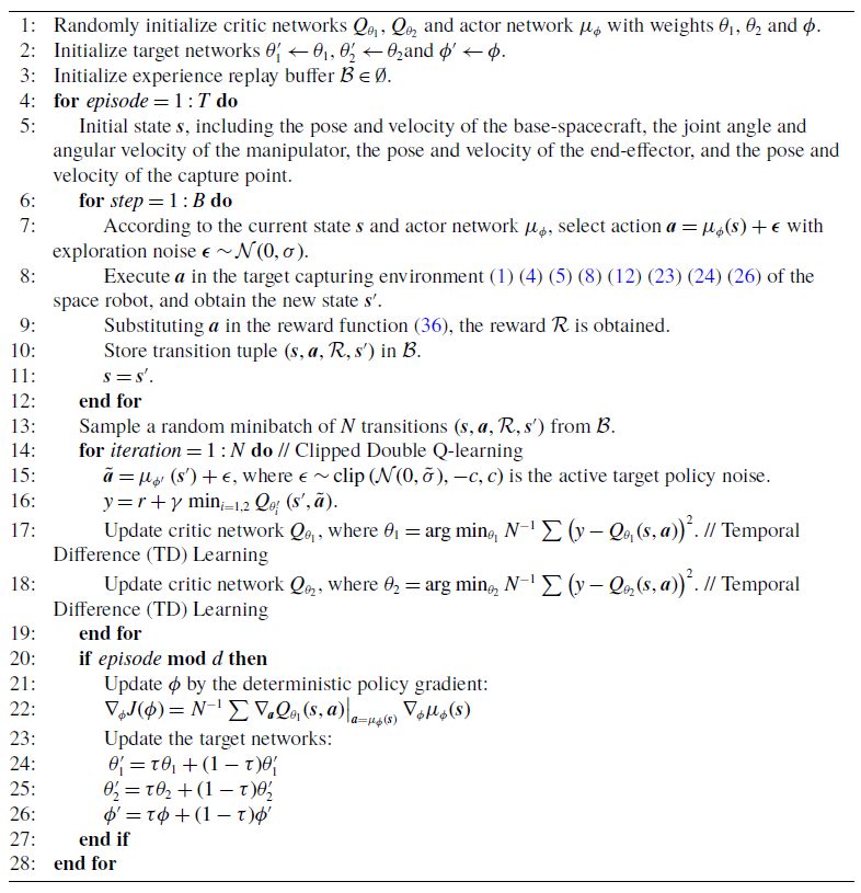
. TD3 learns two Q-functions and uses the smaller one to form the targets in the Bellman error loss functions. The details of the proposed method are presented in Algorithm1. Here,
 $T$
is the maximum number of episodes,
 $B$
is the experience replay buffer length,
 $d$
is the target update frequency, and
 $\tau$
is the target smoothing factor. The target capturing environment in DRL is constructed using the model of the space robot, the model of the tumbling target, and contact dynamics in Section 2.
Trajectory planning method based on DRL TD3

4. Simulation and analysis
4.1. Simulation environment
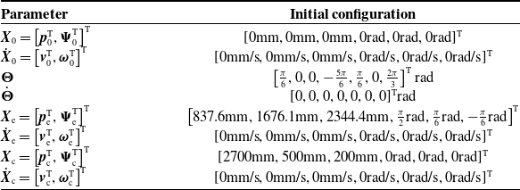
Employing the proposed method, the simulation experiment of a free-floating space robot capturing a non-cooperative tumbling target is conducted. For specific details regarding the mass and inertia of the base-spacecraft, the 7 DOFs manipulator and the non-cooperative tumbling target, and the modified Denavit–Hartenberg (MDH) parameters and joint angle limits of the manipulator, please refer to Appdendix A. Additionally, the initial configuration of the space robot can be found in Table I.
Initial configuration of the space robot.

In the simulation, the CPU model is Intel(R) Core (TM) i7-9700 CPU @ 3.00 GHz, the GPU model is NVIDIA Quadro P2200, and the software is Python. The maximum number of episodes is 5000. The maximum number of steps in each episode is 650 with a step size of 0.2 s. The size of the random experience mini-batch is 500. The number of steps between policy updates is 5. The target smoothing factor is 0.01. The positive constant of the reward function (36) is set to
 $c_1=1$
,
 $c_2=1$
,
 $c_3=\frac {1}{300}$
,
 $c_4=1$
,
 $c_5=\frac {1}{20}$
,
 $c_6=10^{-8}$
,
 $c_7=1$
,
 $c_8=1$
,
 $c_9=1$
,
 $c_{10}=1$
,
 $c_{11}=10$
and
 $c_{12}=10^{-8}$
. The structures of the actor and critic network are shown in Figure 5. In the actor network, the input is
 $\boldsymbol{s} \in \mathbb{R}^{50}$
, and the output is
 $\boldsymbol{a} \in \mathbb{R}^{7}$
. There are four hidden layers, each with 256 neurons, in the actor network. In the critic network, the input is
 $(\boldsymbol{s}, \boldsymbol{a}) \in \mathbb{R}^{57}$
, and the output is the estimation of the expected cumulative long-term reward. There are four hidden layers, each with 512 neurons, in the critic network. In the actor and critic network, the activation function between the hidden layers is the ReLU function. The learning rate for the actor and critic network is 0.001. To prevent violation of constraints (37), the tanh layer and scaling layer are added at the output port. The function of the input
U
and the output
Y
in the tanh layer is established as follows.
 \begin{equation} \boldsymbol{Y}=\tanh (\boldsymbol{U}) \end{equation}
The function of the input U and the output Y in the scaling layer is established as follows.
 \begin{equation} \boldsymbol{Y}=\boldsymbol{k} \cdot \boldsymbol{U}+\boldsymbol{B} \end{equation}
where
 $\boldsymbol{k}=\frac {\overline {\boldsymbol{U}}_{\dot {\boldsymbol{\Theta }}}-\underline {\boldsymbol{U}}_{\dot {\boldsymbol{\Theta }}}}{2}$
is the scaling factor,
 $\boldsymbol{B}=\frac {\overline {\boldsymbol{U}}_{\dot {\boldsymbol{\Theta }}}+\underline {\boldsymbol{U}}_{\dot {\boldsymbol{\Theta }}}}{2}$
is the bias factor,
 $\overline {\boldsymbol{U}}_{\dot {\boldsymbol{\Theta }}}=[0.05,0.05,0.05, 0.05,0.05,0.05,0.05]^{\text{T}}\text{rad/s}$
, and
 $\underline {\boldsymbol{U}}_{\dot {\boldsymbol{\Theta }}}=[\!-0.05,-0.05,-0.05,-0.05,-0.05,-0.05,-0.05]^{\text{T}}\text{rad/s}$
.
Structures of the actor and critic networks.

4.2. Workspace for capturing
To ensure the success of non-cooperative tumbling target capture by the space robot, the workspace of the space robot and the trajectories of the capture point at different initial rotational angular velocities are illustrated in Figure 6. It can be seen that the trajectories of the capture point are always within the workspace of the free-floating space robot, which verifies the feasibility of the capture task.
The workspace of the space robot and the trajectories of the capture point.

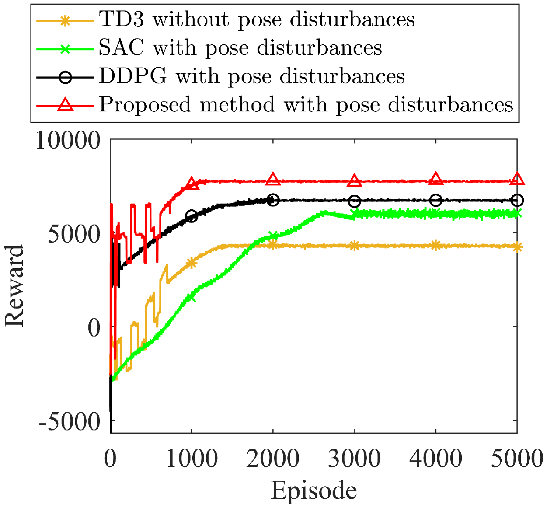
Reward in the training process.

4.3. Simulation results
4.3.1. Performance comparison
In order to evaluate the performance of the proposed method, the simulation of target capture is conducted using the proposed method with pose disturbances, DDPG with pose disturbances, SAC with pose disturbances, and TD3 without base disturbances. The rewards are shown in Figure 7, and the pose disturbances of the base-spacecraft are displayed in Figure 8. Compared the TD3 with and without base disturbances, it can be found that after the introduction of base disturbances, the maximum reward function increased by 79.63%, and the base disturbances error decreased by 50%-96.19%. It can be concluded that the introduction of base disturbances significantly reduced the pose change of the base-spacecraft during capture and effectively improved the tracking accuracy of the space manipulator. Moreover, as seen from Figure 7, SAC, DDPG, and the proposed method reach the maximum reward of 6174.01, 6779.97, and 7623.90 in the 3009, 1754, and 1107 episodes, respectively. Compared with SAC and DDPG, the reward of the proposed method fluctuates in the early episode, but converges faster and obtains a larger learning reward at the end of training. The reason for the fluctuation is that the update of the policy network is delayed, and the weight matrix of the neural network has a large jump every time updated. From Figure 8, it can be seen that compared with SAC and DDPG, during the tracking phase, the peak value of the pose disturbances is reduced by 88.10%, 87.22%, 79.11% and 77.67%, 85.71%, 67.58% in the three translational directions and 70.70%, 72.81%, 45.91% and 77.11%, 50.66%, 50.00% in the three rotational directions, and during the capture phase, 98.7%, 92.9%, 80.7% and 98.8%, 90.6%, 57.6% in the three translational directions and 76.3%, 55.8%, 7.7%, and 60.7%, 55.8%, 15.5% in the three rotational directions. It can be summarized that the proposed method significantly reduces the pose change of the base-spacecraft.
Pose disturbances of the base-spacecraft obtained by the four methods.

4.3.2. Tumbling target capture with different initial rotational angular velocities
In order to evaluate the adaptability of the proposed method, the trained strategy is used to capture the non-cooperative tumbling target with different initial rotational angular velocities
 $\boldsymbol{\omega }_{\mathrm{t}}=[0.5,0.5,0.5]^{\mathrm{T}} {}^{\circ } / \mathrm{s}$
,
 $\boldsymbol{\omega }_{\mathrm{t}}=[1.0,1.0,1.0]^{\mathrm{T}} {}^{\circ } / \mathrm{s}$
, and
 $\boldsymbol{\omega }_{\mathrm{t}}=[1.5,1.5,1.5]^{\mathrm{T}} {}^{\circ } / \mathrm{s}$
, and then the 3D motion trajectories of the end-effector and the capture point and the pose disturbance of the base-spacecraft are illustrated in Figures 9 and 10. In Figure 9, the end-effector pose of the manipulator is continuously adjusted to track the capture point and finally completes the capture. In Figure 10, there is a large peak of the pose disturbance of the base- spacecraft during the tracking process, but the pose disturbance is very small after capture. The above results show that the proposed method can be adopted to tumbling target capture with different initial rotational angular velocities. According to simulation verification, the proposed method can be used to capture tumbling targets with an initial angular velocity of less than 3
 ${}^{\circ }$
/s.
Trajectory of the end-effector and the capture point for capturing the tumbling targets with different initial rotational angular velocities.

Pose disturbance of the base-spacecraft for capturing the tumbling targets with different initial rotational angular velocities.

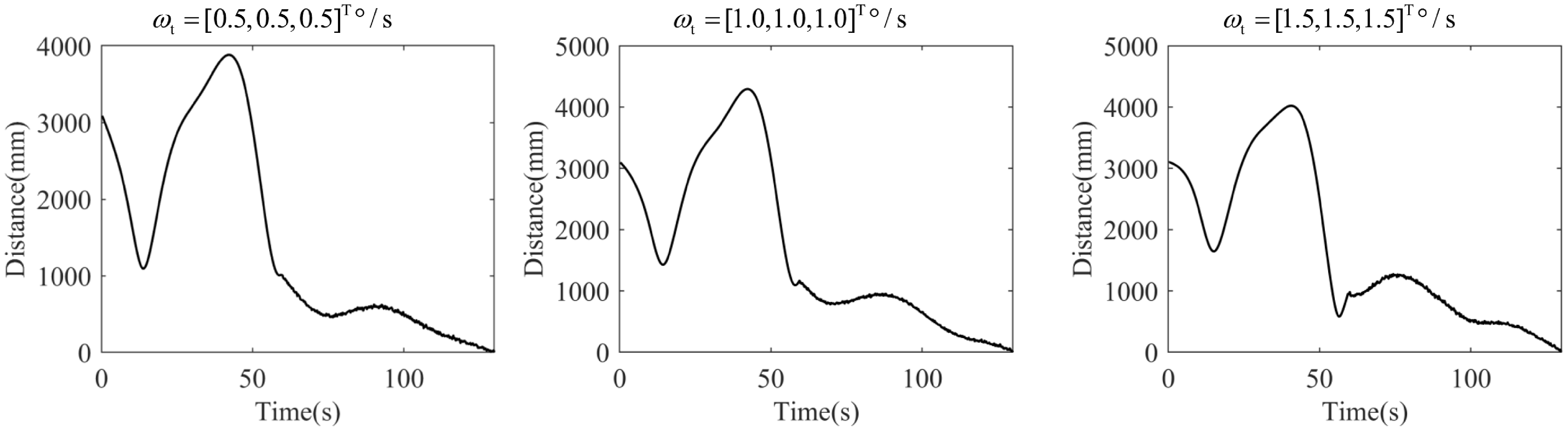
Euclidean distance between the end-effector and the capture point for capturing the tumbling targets with different initial rotational angular velocities.

Joint angle and angular velocity of the space robot.

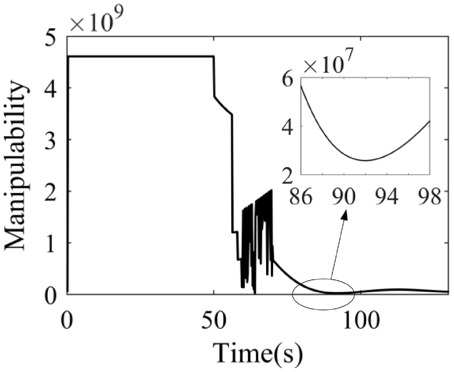
Generalized manipulability of the space robot.

4.3.3. Capture process
To intuitively illustrate the process of capturing the tumbling target, some important evaluation indices are drawn. The Euclidean distances between the end-effector and the capture point are illustrated in Figure 11. The Euclidean distances increased early and then gradually decreased, finally converging to 0.53 mm, 1.89 mm, and 5.23 mm. It shows that the capture accuracy is high, which avoids hard contact between the end-effector and the target. The increase in the distance in the early stage is mainly due to the adjustment of the appropriate configuration of the space manipulator to capture the target with a smaller pose error and a shorter time. In order to clearly show the motion process of the space robot, the joint angles and joint angular velocities of the space robot that capture the non-cooperative target with the initial rotational angular velocities
 $\boldsymbol{\omega }_{\mathrm{t}}=[0.5,0.5,0.5]^{\mathrm{T}} {}^{\circ } / \mathrm{s}$
are shown in Figure 12, and the generalized manipulability of the space robot is given in Figure 13. The angular velocity satisfies the constraint (37), and the joint angle is continuous and within limits. The minimum value of the generalized manipulability is
 $2.350 \times 10^7$
, which is always much greater than 0, indicating that the manipulator is always far away from the singular configuration. There was a slight jitter in 60–70 s because the space manipulator adjusted the end-effector pose by joint 6 to track the capture point.
5. Conclusions
In this paper, the trajectory planning method of the free-floating space robot for non-cooperative tumbling target capture based on TD3 is proposed. The proposed method converges faster with a larger reward and a large generalized manipulability of the space robot. The pose disturbance of the base-spacecraft is reduced due to being added to the reward function. What is more, the proposed method is capable of capturing space non-cooperative tumbling targets with different initial rotational angular velocities. In future work, we will consider planning, tracking, and capturing tumbling targets with irregular geometry and impacted by tiny space debris. In the future, we will conduct in-depth research on collision detection and collision avoidance strategies for space robot capture in combination with mainstream physics engines to improve the feasibility of the proposed method.
Author contributions
Yaqiang Wei and Xinlin Bai designed the study. Yaqiang Wei conducted the experiments and data gathering. Yaqiang Wei and Han Lu performed statistical analyses. Yaqiang Wei wrote the article.
Financial support
This work was supported in part by the Fundamental Research Program of Shenyang Institute of Automation (SIA), Chinese Academy of Sciences under Grant 355060201 and the National Natural Science Foundation of China under Grant 12494562.
Competing interests
The authors declare no conflicts of interest exist.
Ethical Approval
Not applicable.
Appendix
Appendix A. Parameters of the space robot and the target
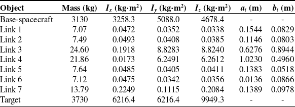
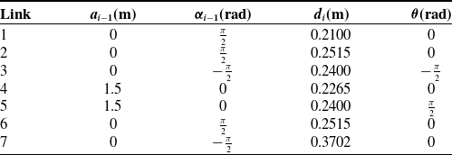
The mass and inertia of the space robot are shown in Table A1, the MDH parameters of the joint coordinate system of the manipulator are shown in Table A2, and the joint angle limits of the space robot are shown in Table A3.
Mass and inertia of the space robot

MDH parameters of the joint coordinate system

Joint angle limits of the space robot