

The subject of social inequality is an important topic for discussion and debate in archaeology (Flannery and Marcus Reference Flannery and Marcus2012; Kintigh et al. Reference Kintigh, Altschul, Beaudry, Drennan, Kinzig, Kohler, Frederick Limp, Maschner, Michener, Pauketat, Peregrine, Sabloff, Wilkinson, Wright and Zeder2014; Kohler and Smith Reference Kohler and Smith2018; Kohler et al. Reference Kohler, Smith, Bogaard, Feinman, Peterson, Betzenhauser, Pailes, Stone, Prentiss, Dennehy, Ellyson, Nicholas, Falseit, Styring, Whitlam, Fochesato, Foor and Bowles2017; Mattison et al. Reference Mattison, Smith, Shenk and Cochrane2016). As noted by Smith and colleagues (Reference Smith, Kohler, Feinman, Kohler and Smith2018), there has been substantial investment in theorizing the topic with significant recent contributions in comparative sociocultural anthropology (e.g., Borgerhoff Mulder et al. Reference Borgerhoff Mulder, Bowles, Hertz, Bell, Beise, Clark, Fazzio, Gurven, Hill, Hooper, Irons, Kaplan, Leonetti, Low, Marlowe, McElreath, Naidu, Nolin, Piraino, Quinlan, Schniter, Sear, Schenk, Smith, von Rueden and Weissner2009; Gurven et al. Reference Gurven, Mulder, Hooper, Kaplan, Quinlan, Sear, Schniter, Rueden, Bowles, Hertz and Bell2010; Smith et al. Reference Smith, Hill, Marlowe, Nolin, Weissner, Gurven, Bowles, Mulder, Hertz and Bell2010). Modeling and comparative anthropology have expanded our understanding of the material conditions favoring the development of social inequality. Archaeologists have also begun to explore the use of rigorous approaches to quantifying inequality in the archaeological record (e.g., Kohler and Smith Reference Kohler and Smith2018, and chapters therein), although, as noted by Smith and colleagues (Reference Smith, Kohler, Feinman, Kohler and Smith2018), this has not yet been common. One of the major challenges for archaeologists in devising tests of hypotheses concerning inequality (or virtually any other cultural phenomenon) is having sufficient resolution in the record to adequately explore the nuances of model predictions.
The evolution of material wealth-based inequality has been the subject of intensive research and ongoing debate in the Middle Fraser Canyon of interior British Columbia (Harris Reference Harris2012; Hayden Reference Hayden, Burch and Ellana1994, Reference Hayden1997, Reference Hayden1998; Prentiss and Kuijt Reference Prentiss and Kuijt2012; Prentiss et al. Reference Prentiss, Chatters, Lyons and Harris2011); it is now clear that material wealth-based inequality measurable on an inter-house basis appeared in the Middle Fraser during the period of 1300–1000 cal BP when large aggregate villages were at peak size (Prentiss et al. Reference Prentiss, Lyons, Harris, Burns and Godin2007, Reference Prentiss, Cross, Foor, Markle, Hogan and Clarke2008, Reference Prentiss, Foor, Cross, Harris and Wanzenried2012, Reference Prentiss, Cail and Smith2014; Prentiss, Foor, and Hampton Reference Prentiss, Foor and Hampton2018; Prentiss, Foor, and Murphy Reference Prentiss, Foor, Murphy, Kohler and Smith2018). This came at a time of evident economic hardship following a time of rapid growth. What remains unclear is the exact time when unequivocal inequality first appears in reference to relationships between population growth, the onset of subsistence stress, and subsequent demographic decline. Definition of this time line is essential for testing more nuanced explanatory models for understanding emergent inequality. Archaeologists have also been unclear as to whether inequality extended to family relations within houses. Hayden (Reference Hayden1997) and Lepofsky and colleagues (Reference Schiffer1996) have argued such a case for the well-known Keatley Creek site in interior British Columbia. Research at Bridge River has until recently emphasized inter-house patterns. This is an important problem as our understanding of the inequality process depends on insight as to how individual families interacted, whether as household cooperatives or as collectives semi-independently engaged in struggle for their own unique social position and thus long-term survival.
In this article, we rely on the record of Housepit 54 at the Bridge River site (EeRl4) to test hypotheses about the advent of persistent material wealth-based inequality. We accomplish this by assessing evidence for inter-floor variation in measurable material wealth and comparing those outcomes to measures of population, subsistence productivity, and cooperation. The outcome suggests that inequality indeed did emerge on the late floors of Housepit 54 and is correlated with population trends and changes in patterns of cooperation. This offers important implications for both our theoretical understanding of emergent inequality and for our interpretation of long-term indigenous (St’át'imc) history.
Theorizing the Evolution of Social Inequality
In a recent assessment of inequality research in archaeology, Smith and colleagues (Reference Smith, Kohler, Feinman, Kohler and Smith2018) point to three major topics: How did it originate? How did it persist? How is variation explained? This study examines the first of these, the origination of inequality. This topic has been of long-standing interest to anthropologists (e.g., Durkheim Reference Durkheim2014 [1893]) but has only developed as a central focus for archaeologists in recent decades. A substantial quantity of ethnographic and archaeological work (e.g., Borgerhoff Mulder et al. Reference Borgerhoff Mulder, Bowles, Hertz, Bell, Beise, Clark, Fazzio, Gurven, Hill, Hooper, Irons, Kaplan, Leonetti, Low, Marlowe, McElreath, Naidu, Nolin, Piraino, Quinlan, Schniter, Sear, Schenk, Smith, von Rueden and Weissner2009; Flannery and Marcus Reference Flannery and Marcus2012; Gurven et al. Reference Gurven, Mulder, Hooper, Kaplan, Quinlan, Sear, Schniter, Rueden, Bowles, Hertz and Bell2010; Kohler and Smith Reference Kohler and Smith2018; Kohler et al. Reference Kohler, Smith, Bogaard, Feinman, Peterson, Betzenhauser, Pailes, Stone, Prentiss, Dennehy, Ellyson, Nicholas, Falseit, Styring, Whitlam, Fochesato, Foor and Bowles2017, Reference Kohler, Smith, Bogaard, Peterson, Betzenhauser, Feinman, Oka, Pailes, Prentiss, Stone, Dennehy, Ellyson, Kohler and Smith2018; Mattison et al. Reference Mattison, Smith, Shenk and Cochrane2016; Smith et al. Reference Smith, Hill, Marlowe, Nolin, Weissner, Gurven, Bowles, Mulder, Hertz and Bell2010) has explored the wide range of conditions that are thought to favor the emergence of inequality. Mattison and colleagues (Reference Mattison, Smith, Shenk and Cochrane2016) summarize this information and point to a specific set of factors associated with the onset of what they term persistent institutionalized inequality (PII) defined as “differential access to power or resources involving institutionalization of status hierarchies by hereditary privileges or positions such as social classes, castes, hereditary titles, or heritable differences in wealth” (2016:185). For purposes of this article, we consider PII to be present when there is archaeological evidence for transmission of material wealth, opportunities to build wealth, and/or rights to wealth that persist across two or more generations. Our primary interest is in the evolutionary development of this phenomenon, and thus we are less concerned with variability in its persistence, though our data offer some insights therein.
Many models have been developed to explain the development of social strategies that include accumulation and transmission of wealth within the Pacific Northwest region. We examine the three most prominent in light of differences in assumptions and test expectations. The first model assumes that wealth accumulation and transmission and the associated emergent inequality are fundamentally adaptive. Hayden's (Reference Hayden, Burch and Ellana1994, Reference Hayden, Price and Feinman1995, Reference Hayden1997, Reference Hayden1998) aggrandizer model is the best representative of this approach. Hayden offers a simple formula in which productive resources, plus the ubiquitous presence of obsessively self-driven men known to Hayden as aggrandizers, will quickly lead to inequality. Hayden (Reference Hayden, Price and Feinman1995) argues that ascendant aggrandizers will employ different strategies for achieving wealth and influence depending on local subsistence resource structure. Hayden and Ryder (Reference Hayden and Ryder1991; Hayden et al. Reference Hayden, Bakewell and Gargett1996) view such strategies as highly adaptive and thus prone to persist in contexts with resources resistant to overexploitation (e.g., river valleys with major salmon runs). Most critical to such a scenario is the assumption that aggrandizers are born in all societies, and that they simply need the right conditions (resource abundance) and technologies to engage in wealth- and status-building schemes. Once initiated, aggrandizer strategies are expected to be rewarded with cooperative social units, economic productivity, and population growth.
An alternative collection of models assumes that practices associated with inequality are adaptive, although their manifestation is dependent on population dynamics. Various scholars have linked population size and adaptive payoffs for investing in managers to avoid societal breakdown and group fissioning (e.g., Ames Reference Ames, Price and Brown1985; Bandy Reference Bandy2004; Friesen Reference Friesen1999; Johnson Reference Johnson, Renfrew, Rowlands and Segraves1982; Smith and Choi Reference Smith, Choi, Kohler and van der Leuw2007). In these scenarios, groups make choices as to how to best manage information associated with growing numbers of people and the associated challenges of managing an increasingly complicated economy. Once leadership is established, leaders gain the opportunity to develop respect and also the possibility of accumulating wealth as a marker of position. None of these models require the presence of individuals with genetically predisposed sociopathic personality types. These models should be supported by correlations between wealth markers, population size, economic productivity, and intra-network cooperation in labor.
A third model recognizes emergent inequality as a byproduct of competitive conditions associated with population and resource imbalances. Malthusian demographic models point to the possibility of inequality emerging from competition developing during food crises triggered by imbalances between population and food production capacity (Lee et al. Reference Lee, Puleston and Tuljapurkar2009; Prentiss et al. Reference Prentiss, Cail and Smith2014; Puleston and Tuljapurkar Reference Puleston and Tuljapurkar2008; Winterhalder et al. Reference Winterhalder, Puleston and Ross2015). Inequality within such contexts could emerge as patron-client relationships developed between those with greater and lesser economic success in the new environment (e.g., Boone Reference Boone, Smith and Winterhalder1992; see also Arnold Reference Arnold1993, Reference Arnold1996; Prentiss et al. Reference Prentiss, Lyons, Harris, Burns and Godin2007, Reference Prentiss, Foor, Cross, Harris and Wanzenried2012). If persistent across generations, such relations would come to reflect institutionalized material wealth-based inequality. Cultural practices within such scenarios may be differentially adaptive depending on individual and group performance, but overall such a scenario reflects a population coping with severe subsistence stress that may only persist or return to a growth phase with the injection of new food resources or significant loss of population (Lee et al. Reference Lee, Puleston and Tuljapurkar2009; Puleston and Tuljapurkar Reference Puleston and Tuljapurkar2008). Thus, inequality would emerge in what is defined as the Malthusian transition period immediately preceding a full-on Malthusian ceiling (Puleston et al. Reference Puleston, Tuljapurkar and Winterhalder2014) and persist until interrupted by a shift in resource productivity or complete loss of population either by mortality or emigration (if an option). The Malthusian transition period could be the culmination of either rapid population growth or immigration of other peoples into a constrained population space. Regardless of how it emerges, imbalance between population and resources leads to sustained stress in subsistence production and as conditions become severe, previous cooperation networks break down (though new alliances could temporarily form as well [e.g., Winterhalder Reference Winterhalder1986]).
Studying the Emergence of Material Wealth-Based Inequality at the Bridge River Site
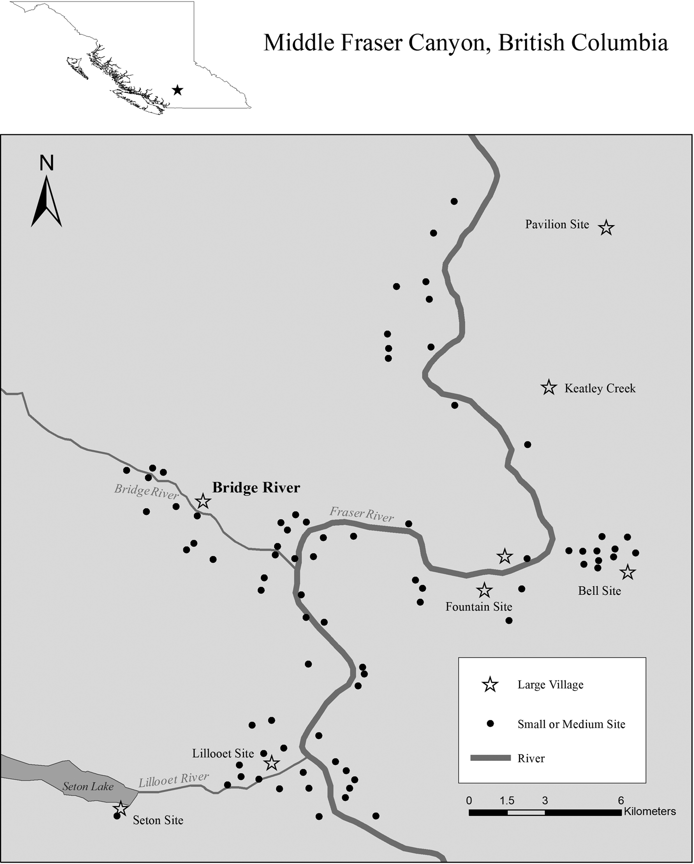
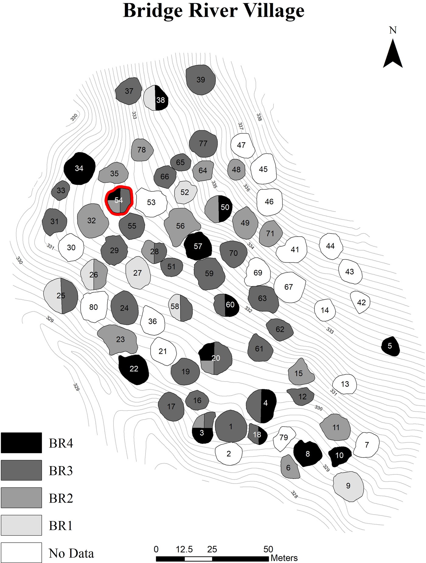
The Bridge River site (EeRl4), located in the Bridge River Valley approximately 2 km from the Six-Mile Rapids fishery in Middle Fraser Canyon, is one of several large housepit villages (Figure 1) that have become central to discussions and debates regarding the emergence of material wealth-based inequality (Hayden Reference Hayden, Burch and Ellana1994, Reference Hayden1997; Hayden and Spafford Reference Hayden and Spafford1993; Hayden et al. Reference Hayden, Bakewell and Gargett1996; Prentiss and Kuijt Reference Prentiss and Kuijt2012; Prentiss, Foor, and Murphy Reference Prentiss, Foor, Murphy, Kohler and Smith2018; Prentiss et al. Reference Prentiss, Lyons, Harris, Burns and Godin2007, Reference Prentiss, Chatters, Lyons and Harris2011, Reference Prentiss, Foor, Cross, Harris and Wanzenried2012, Reference Prentiss, Cail and Smith2014). The site was test excavated by Stryd (Reference Stryd1974) who drew initial conclusions regarding the scale of the village and time depth of its occupation. Intensive research by our teams since 2003 has clarified aspects of village history. Initial geophysical mapping and subsequent testing permitted the establishment of radiocarbon histories for 55 of the site's 80 housepits (Prentiss et al. Reference Prentiss, Cross, Foor, Markle, Hogan and Clarke2008). A critical outcome of that work was recognition that, unlike many other sites, including the Keatley Creek site (Hayden Reference Hayden1997, Reference Hayden2000; Prentiss et al. Reference Prentiss, Lenert, Foor, Goodale and Schlegel2003, Reference Prentiss, Lyons, Harris, Burns and Godin2007), the Bridge River housepits contained well-preserved multifloor sequences. This has provided the opportunity to develop a model of village-wide evolution drawing from composite household histories. Most broadly, the village developed in four occupation periods: BR1 (ca. 1800–1600 cal BP), BR2 (ca. 1600–1300 cal BP), BR3 (ca. 1300–1000 cal BP), and BR4 (ca. 500–100 cal BP). The occupation pattern in the BR1 period is not well understood but likely consisted of one or more small clusters of housepits of variable size. There was rapid growth at the start of BR2 times, leading to what appears to have been two concentric rings of houses stretching across the breadth of the village core (Prentiss and Walsh Reference Prentiss, Walsh and Sanz2018; Figure 2). Current data suggest that most of the BR2 houses were abandoned in the late BR2 period, with only three (including Housepit 54) crossing the boundary into BR3 times. The BR3 period was initiated with very rapid population growth, culminating in the establishment of contiguous ring-like clusters of houses (Figure 2). After achieving peak numbers in early-mid BR3 (ca. 1200–1300 cal BP), houses were steadily abandoned, with complete village abandonment occurring by about 1000 cal BP. This is similar to patterns with wider abandonments of large aggregate villages throughout the Mid-Fraser region (Hayden and Ryder Reference Hayden and Ryder1991; Kuijt Reference Kuijt2001; Kuijt and Prentiss Reference Kuijt, Prentiss, Prentiss and Kuijt2004). The village was reoccupied in the late precolonial period and into the British Columbia Fur Trade period. Housepit 54 was evidently the final house occupied during the latter time (cal AD 1853–1858; Prentiss, ed. Reference Prentiss2017).
Map of Middle Fraser Canyon area showing major sites. Map by Ethan Ryan.

Map of Bridge River site showing distribution of housepits occupied during the BR1–4 periods. Differential shading only marks occupation of the house during different Bridge River occupation periods. It does not refer to length of time or intensity of occupation. Map by Ethan Ryan.

The BR3 period offers evidence for emergent wealth-based inequality under conditions of developing subsistence stress. Sample excavations of six BR2 and BR3 housepits revealed a variety of indicators of material wealth-based inequality (Prentiss et al. Reference Prentiss, Foor, Cross, Harris and Wanzenried2012, Reference Prentiss, Cail and Smith2014, Reference Prentiss, Goodale, Harris, Crossland, Goodale and Andrefsky2015). A range of additional evidence suggested that beginning in mid-BR3 times, the village population suffered from subsistence stress associated with a Malthusian ceiling event (Prentiss, Foor, and Hampton Reference Prentiss, Foor and Hampton2018; Prentiss et al. Reference Prentiss, Cail and Smith2014). Densities of salmon and deer remains decline between the BR2 and BR3 periods. Deer remains during BR3 times are also more intensely processed and generally derive from appendicular portions, likely reflecting greater field processing to reduce transport costs (e.g., Janetski Reference Janetski1997). Data from Keatley Creek also implicate the effects of subsistence stress at this time. Evidence from Housepit 7 at that site suggests that as salmon numbers declined, diet breadth expanded, with the addition of a wider range of mammal species added to the diet. Furthermore, faunal and botanical data suggest that over time, household members had to hunt and gather at increasing distances to access critical foods (Prentiss et al. Reference Prentiss, Lyons, Harris, Burns and Godin2007). These patterns come at a time when marine productivity evidently declined (Hay et al. Reference Hay, Dallimore, Thomson, Calvert and Pienetz2007; Hutchinson et al. Reference Hutchinson, Butler, Campbell, Sterling, Etnier and Bovy2018; Patterson et al. Reference Patterson, Prokoph, Kumar, Chang and Roe2005; Tunnicliffe et al. Reference Tunnicliffe, O'Connell and McQuoid2001; Wright et al. Reference Wright, Dallimore, Thomson, Patterson and Ware2005), and salmon abundance was reduced not just in the Fraser and Thompson Rivers but also in the Columbia (Chatters et al. Reference Chatters, Butler, Scott, Anderson and Neitzel1995). The timing of reduced marine, and by proxy, salmon productivity, was very poor for Mid-Fraser peoples, whose total numbers may have peaked at over 8,000 persons within an approximately 20 km stretch of the Fraser River during the early BR3 period (Prentiss et al. Reference Prentiss, Cail and Smith2014). The combination of high demographic numbers and declining interannual access to keystone resources made for a rapid reversal from a copial, or growth, cycle to a Malthusian transition and ceiling period (henceforth described as the Malthusian period).
The Record from Housepit 54
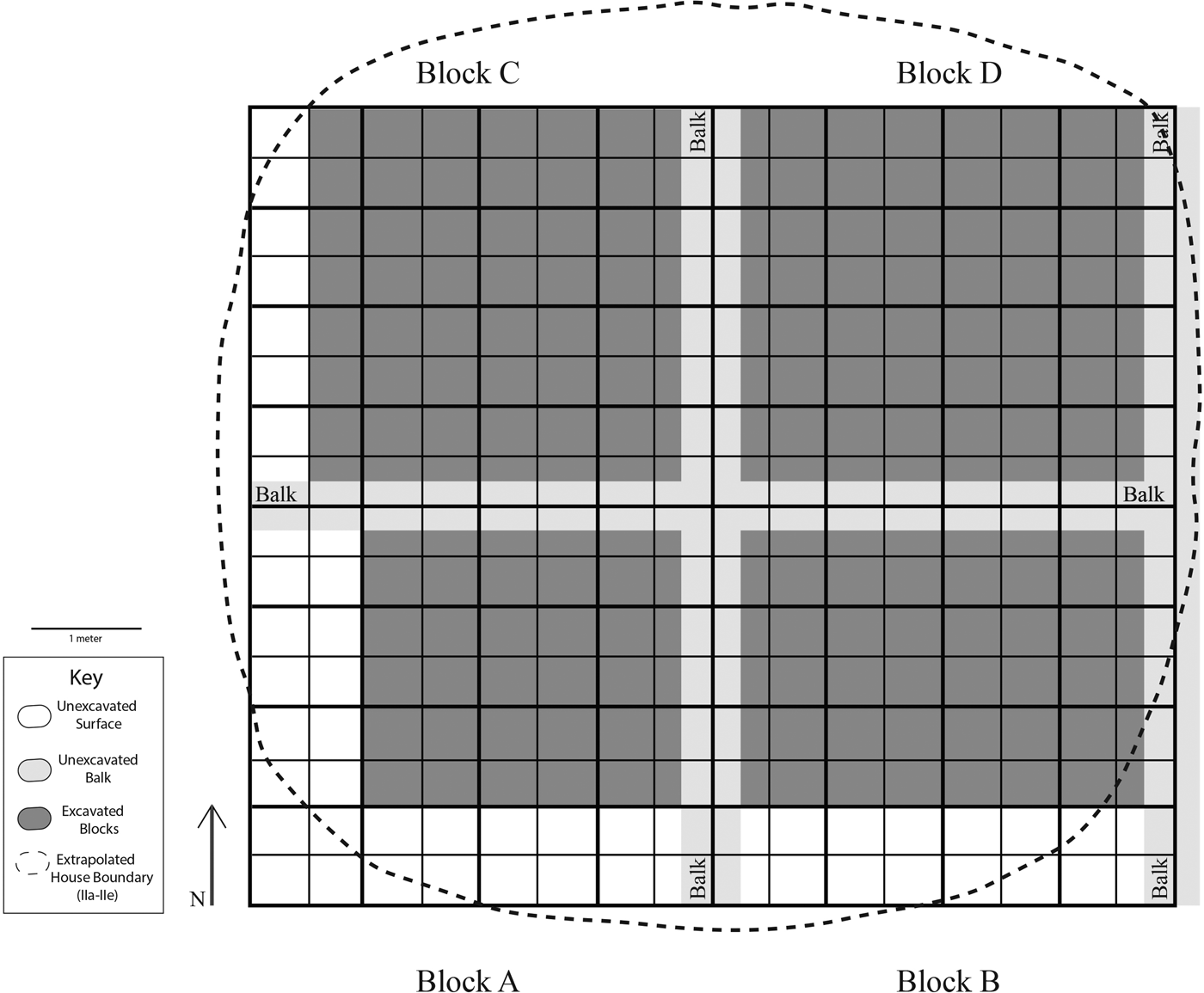
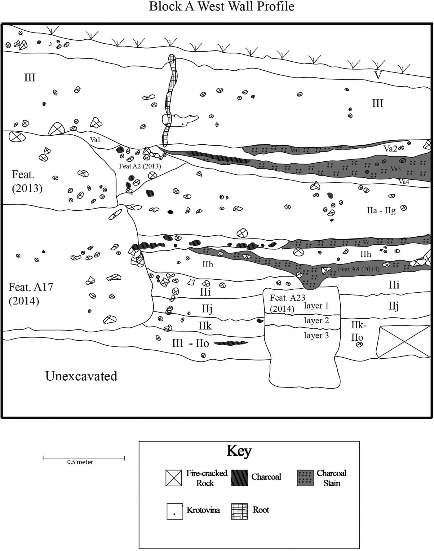
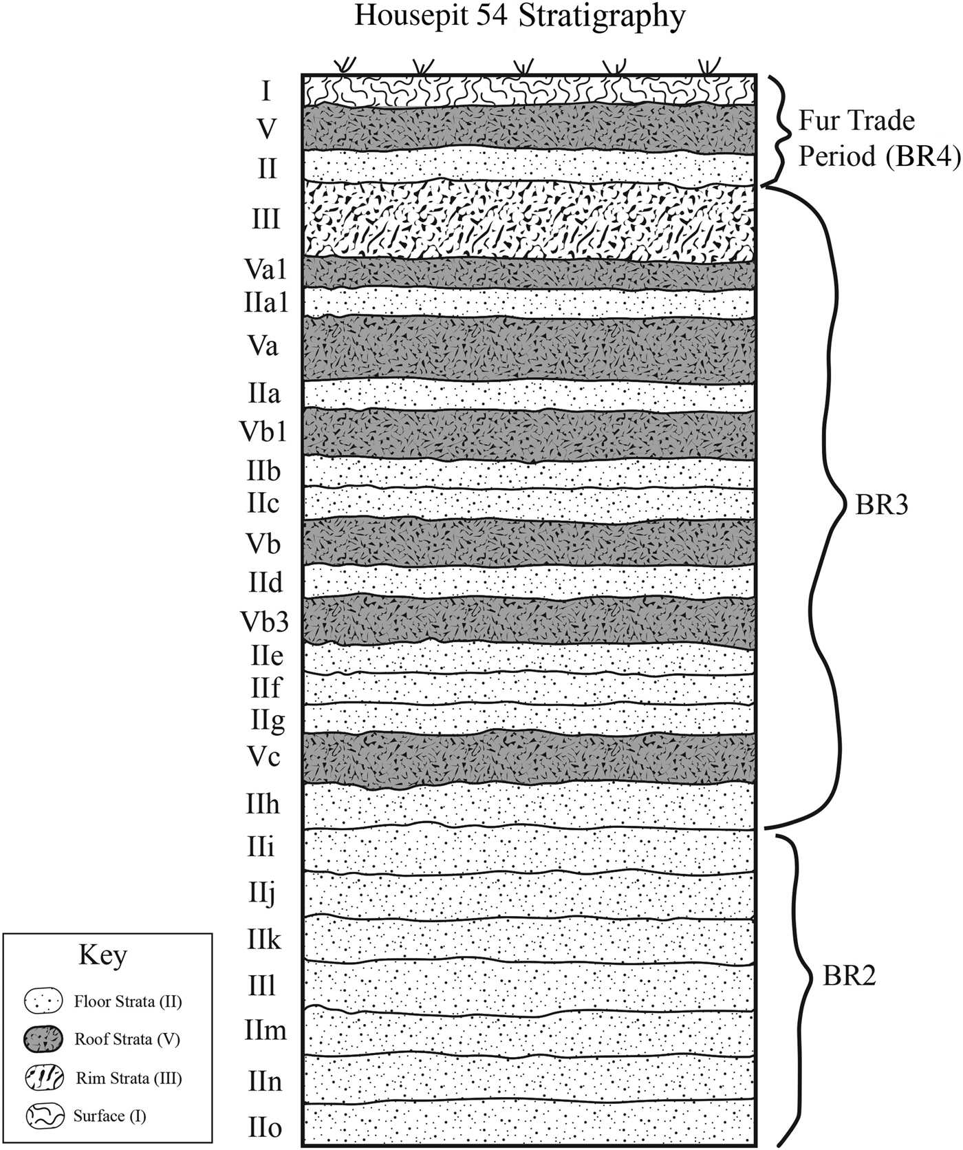
Housepit 54 was first identified as having a unique and potentially long record during test excavations in 2004 and 2008 (Prentiss et al. Reference Prentiss, Cross, Foor, Markle, Hogan and Clarke2008, Reference Prentiss, Foor, Cross, Harris and Wanzenried2012). Consequently, our research team determined that with 17 well-preserved anthropogenic floors, this housepit would be ideal for addressing questions concerning the role of intra-house dynamics during the majority of the occupation periods at Bridge River (Prentiss, Foor, and Hampton Reference Prentiss, Foor and Hampton2018). Excavations from 2012 to 2016 focused on exposure of nearly entire floor surfaces for each floor using a system of 4 × 4 m blocks, 1 × 1 m units, and 50 × 50 cm quads (Figure 3). The floors are composed of human-transported clay loam with small gravels derived from the sedimentary substrate below and around the Bridge River village, then mixed with microscopic products of human-related activity (e.g., crushed bone) and mildly bioturbated by insects and plant roots (Goldberg Reference Goldberg2010). Each successive floor was identified by the presence of a somewhat “greasy” surface typically containing abundant fish remains and artifacts lying horizontally along with features that included hearths and cache pits. Strata were defined by standard Roman numeral designations that included site surface (I), floor (II), housepit rim midden (III), substrate (IV), and roof (V). A range of additional stratigraphic designations were developed for more rare sediment types expressed across the site. Letter designations were added for repeated sediment types. Thus, the floor sequence at Housepit 54 included stratum II, the Fur Trade period floor, and then floors IIa through IIo with earlier dates (Figure 4). Several roof strata were also identified, although only two had significant deposits (the Fur Trade period roof [V] and the final BR3 roof capping floor IIa [Va]). All sediments not collected for flotation and geochemical analysis were sieved through ⅛-inch mesh screens and excavator screens were checked by Prentiss. Excavators were also instructed to point provenience all artifacts, faunal remains, and fire-cracked rock (the latter greater than 3 cm maximum diameter) when excavating floors. Details regarding stratigraphy and chronology have been published elsewhere (Prentiss, Foor, and Hampton Reference Prentiss, Foor and Hampton2018), but briefly, the IIa–IIo sequence provided a continuous series of reoccupations spanning 1100–1460 cal BP, reflecting occupations averaging 23 years, or about a generation, each. The floors of Housepit 54 varied in size over time (Figure 5; Supplemental Figures 1–3). The earliest three floors (IIm–o) reflect what appear to be smaller single family structures. Floors IIf through IIl represent a rectangular-shaped house with what appear to be two major activity areas. Floors IIa through IIe represent the full-sized house reflected by the house depression on the site surface. Our maps (Supplemental Figures 1–3) illustrate the extent of each floor. However, the roofs associated with floors IIa–IIl probably extended up to 2 m over an earthen bench-like space above the floor level, making the functional interior spaces more substantial than what is depicted in our maps. The extra above-floor/bench space would have been used for a variety of functions, including sleeping and storage. All floors have what appear to be major activity spaces containing varying combinations of hearths, hearth-cleanout, cache pits, discarded artifacts, and food remains. The Block D, or northeast quarter, of floor IIa was not occupied but instead was used as a refuse area connected with the house rim deposits. Given this date range and growth history, Housepit 54 provides an ideal context to examine household dynamics between middle BR2 and late BR3 times. We recognize, however, that while the record of Housepit 54 offers the potential for significant new insights, it is only one house among many and could reflect a unique trajectory. We return to this concern in the discussion section.
Housepit 54 excavation grid. Dark shading shows areas targeted for excavation. Details regarding actual extent of excavation on a floor by floor basis are provided in Prentiss, Foor, and Hampton (Reference Prentiss, Foor and Hampton2018). Figure by Ashley Hampton.

West wall profile from Block A, Housepit 54, showing major strata. Figure by Ashley Hampton from an original drawing by Anna Marie Prentiss.

Summary stratigraphic profile (not to scale) of Housepit 54 illustrating complete sequence of strata inclusive of surface (I), rim-midden (III), roofs (V), and floors (II). Plan views of the IIa–IIo floor sequence emphasizing feature distributions are found in Supplemental Figures 1–3. Plan views of the same floors illustrating all point-provenienced features, artifacts, and faunal remains can be found in Prentiss, Foor, and Hampton (Reference Prentiss, Foor and Hampton2018). Figure by Ashley Hampton.

Analysis
Data from the 15 BR2 and BR3 period floors at Housepit 54 can be used to test three hypotheses regarding the evolution of material wealth-based inequality, and this requires several steps. First, we establish consistency in the residential occupations of Housepit 54. Second, we test for the presence of inequality between the floors of Housepit 54. Third, we establish the history of population and food storage across the Housepit 54 floors. Fourth, we develop a measure of labor variation that we use to determine the likelihood of change in cooperation between inhabitants of each floor in Housepit 54. Ultimately, we examine relationships among these data to assess predictions associated with the three hypotheses.
Occupation Consistency
Mid-Fraser pithouses were typically winter residences (Prentiss and Kuijt Reference Prentiss and Kuijt2012). However, they were also places where house members could reside any time of year. It is well-known that people came and went from their houses during the warm season, as resources from different sectors within their environment were acquired and placed within the house for later use (Alexander Reference Alexander and Hayden1992, Reference Alexander and Hayden2000). Furthermore, it is also possible that the infirm and/or extremely elderly could remain in and around the house during the warm season, while most house members were engaged in fishing, hunting, and gathering activities in the surrounding environment (Alexander Reference Alexander and Hayden2000; Prentiss and Kuijt Reference Prentiss and Kuijt2012). Thus, it is easy to imagine scenarios where in a given year a house might be periodically used for short-term visits and never receive a full-term winter occupation. If this were the case, then accumulated artifacts could reflect quite different contingencies from regular winter occupations with their wide array of food preparation and manufacture work (Alexander Reference Alexander and Hayden2000; French Reference French and Prentiss2017; Prentiss and Kuijt Reference Prentiss and Kuijt2012; Prentiss et al. Reference Prentiss, French, Hocking, Mattes, Walsh, Bobbitt, Barnett and Prentiss2017). Alternatively, inter- and intra-floor variability in the distribution of discarded lithic artifacts could also be affected by differential cleaning (e.g., Schiffer Reference Schiffer1972, Reference Schiffer1983; Stevenson Reference Stevenson1982, Reference Stevenson1985). Our research on formation processes has to date shown that floors were not swept or otherwise cleaned to any significant degree and thus appear to reflect in situ debris from household activities (Prentiss, Foor, and Hampton Reference Prentiss, Foor and Hampton2018; Ryan Reference Ryan2018).
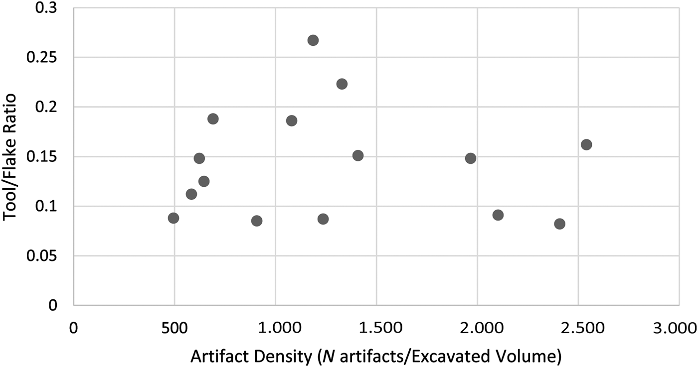
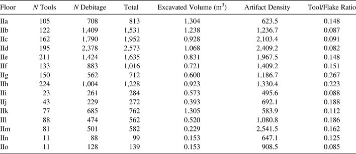
We used two approaches to measuring occupational consistency at Housepit 54. First, we assessed inter-floor variability in occupation length using techniques explicated by Kuhn and Clark (Reference Kuhn and Clark2015) for examining the same phenomena in Paleolithic cave contexts. A plot of lithic tool to flake ratio against artifact density is useful in assessing occupation intensity. Ideally, short-term visits to a living space should generate low-density assemblages characterized by high tool/flake ratios. In contrast, longer-term occupations, typical of residences, should have higher densities of artifacts and should have much lower tool/flake ratios, given increasing investment in tool manufacture and maintenance. We calculated tool/flake ratios and artifact densities for all Housepit 54 floors, and the results illustrate consistently low tool/flake ratios against variable artifact densities (Table 1; Figure 6). The higher tool/flake ratio scores come from floors with excessively high ground stone artifact frequencies. Comparing our results to those of Kuhn and Clark (Reference Kuhn and Clark2015), it is clear that our data reflect consistency on the residential end of the spectrum.
Tool/flake ratio plotted against artifact density.

Tool/Flake Ratio and Total Artifact Density Data.

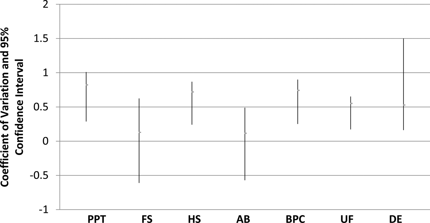
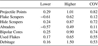
We also tested for occupational intensity by calculating coefficients of variation (COV) on frequencies of major tool classes (projectile points, flake scrapers, hide scrapers, abraders, bipolar cores, used flakes, and debitage). We then plotted the results along with 95% confidence intervals to assess the significance of variation between classes (Kuhn and Clark Reference Kuhn and Clark2015). The assumption here is that if occupations were variable resulting from short-term visits along with occasional longer stays, then COV scores would be higher on tools and debitage. In contrast, if the floors were consistently occupied as residential spaces with a standard set of activities, then the only aspect that would vary would be the intensity of lithic reduction, and thus COV scores would be consistently low for tools while debitage could score higher. Results indicate consistently low COV scores and overlapping confidence intervals (Table 2; Figure 7). Interestingly, debitage have an equivalent COV but a comparatively wide confidence interval, which again supports the residential consistency argument.
Coefficient of Variation and 95% confidence intervals for major tool classes (those with N > 100) from Housepit 54 (PPT = Projectile Point; FS = Flake Scraper; HS = Hide Scraper; AB = Abrader; BPC = Bipolar Core; UF = Used Flake; DE = Debitage).

Coefficient of Variation (COV) and 95% Confidence Interval Range on Highest Quantity (N > 100) Artifact Classes from Housepit 54.

A second consistency issue concerns activity areas on floors. Mid-Fraser house floors were occupied using two quite different occupational strategies. Ethnographies of groups on the Canadian Plateau indicate that houses were communally organized with designated zones for cooking or tool making, sleeping, and socializing (Teit Reference Teit1900, Reference Teit1909). The same pattern was found on the Fur Trade period floor of Housepit 54 (Barnett and Frank Reference Barnett, Frank and Prentiss2017; Williams-Larson et al. Reference Williams-Larson, Barnett, Yu, Schmader, Prentiss and Prentiss2017). In contrast, Lower Lillooet (Lil'wat) house floors were organized by domestic units spaced evenly around the periphery of the house floor with an open central space for communal activity and movement around the house. This pattern has been commonly recognized in larger housepits excavated in the Middle Fraser Canyon that predate about 1000 BP (Hayden and Spafford Reference Hayden and Spafford1993; Lepofsky et al. Reference Lepofsky, Kusmer, Hayden and Lertzman1996). We tested for activity area consistency drawing from method and theory in multivariate reliability testing (Carmines and Zeller Reference Carmines and Zeller1979). More specifically, we developed a principal components analysis (PCA) using IBM SPSS Version 24 of a data matrix consisting of all excavated blocks from all floors by a 17-variable list of major tool classes (Supplemental Table 1). Following Carmines and Zeller (Reference Carmines and Zeller1979; see also Prentiss Reference Prentiss1998), acceptable reliability (or consistency) is indicated by a first principal component capturing 40% or more of the total variance and an unrotated loading matrix that includes positive loading by the majority of variables at 0.3 or better. We also calculated a summary reliability statistic known as coefficient theta from the results of the PCA (Carmines and Zeller Reference Carmines and Zeller1979). A theta score of 0.8 or better is widely assumed to mark acceptable reliability and thus consistency (Nance and Ball Reference Nance and Ball1986; Prentiss Reference Prentiss1998).
The PCA produced four significant components, with the first capturing approximately 41% of the total variance (Supplemental Tables 2–6). The first component contained strong positives scores on 13 of the 17 variables. We calculated a coefficient theta score of 0.857. These results suggest that with a small range of error variability, artifact assemblages are consistent and represent a wide range of activities in each area of each floor. To further explore the PCA outcome, we calculated a correlation coefficient on the relationship between the first component scores and assemblage size. Results suggest that variation in the contribution of the cases to the first component is strongly related to sample size (r = 0.815; p = 0.01). Consequently, we conclude that activity areas are consistently multi-activity domestic areas that vary primarily due to activity intensity (rather than activity type).
Assessing Inequality on Housepit 54 Floors
Clearly, Housepit 54 was occupied throughout its lifespan by residential groups. Our next task is to determine if at some point a pattern of intra-house material wealth-based inequality developed. We have established the high likelihood that each floor in the IIa to IIl range was occupied by collectives consisting of two or more domestic groups conducting activities in and around hearth features. It is not unreasonable to explore the possibility that these domestic groups acted autonomously at times, thus creating the opportunity for differential success in household production and variability in social networking for exchange purposes. Such patterns are well-known from houses associated with Wakashan and Coast Salish groups on the central Northwest Coast with similar spatial constraints on living spaces for family units (Chatters Reference Chatters, MacEachern, Archer and Garvin1989; Coupland et al. Reference Coupland, Clark and Palmer2009; Drucker Reference Drucker1951; Samuels Reference Samuels, Sobel, Ann Trieu Gahr and Ames2006). This pattern has also been identified in more interior British Columbia contexts as, for example, among the Lil'wat who resided to the southwest of the Mid-Fraser area (Teit Reference Teit1906). Finally, collectivist household organization has been widely inferred from an archaeological standpoint in the Mid-Fraser area (e.g., Hayden and Spafford Reference Hayden and Spafford1993; Lepofsky et al. Reference Lepofsky, Kusmer, Hayden and Lertzman1996; Smith Reference Smith and Prentiss2017). Ideally, inequality would be assessed using measures such as the Gini coefficient (e.g., Kohler and Smith Reference Kohler and Smith2018) calculated as a measure of intra-floor variation. Prentiss, Foor, and Murphy (Reference Prentiss, Foor, Murphy, Kohler and Smith2018) made use of Gini coefficients to assess variability in subsistence and wealth measures on the IIa–IIe floors of Housepit 54. That study determined that the majority of Ginis achieved high scores on the IIc floor. A drawback to that study was our inability to test for inequality using Gini coefficients on the deeper floors given insufficient numbers of activity areas from which to measure diversity on the deeper floors (IIf–IIo). If we seek to identify variation in wealth between domestic areas through the majority of the Housepit 54 strata, then we need to employ a different strategy. Prentiss and colleagues (Reference Prentiss, Foor, Cross, Harris and Wanzenried2012) used PCA to define co-associations between multiple measures of wealth accumulation across multiple housepits at Bridge River. Component scores were then used to assess degree of wealth accumulated in each house. This approach can be used to examine variability in wealth markers on the Housepit 54 floors.
We developed five measures drawing entirely on the lithic artifact assemblages from Housepit 54. Non-local raw material density permits us to assess the degree to which domestic groups engaged in either exchange with other community members or were permitted toolstone collection in neighboring territories. Non-local raw materials in this study consist of obsidian, a number of cherts (specifically jasper, Hat-Creek jasper, and pisolite), and chalcedonies not known to be found in the Bridge River valley (Crossland and McKetta Reference Crossland and McKetta2007; Rousseau Reference Rousseau and Hayden2000). A general chert class was not included as many are not well sourced. Prestige raw material density concerns the accumulation of toolstone generally associated with the production of highly valued ornaments and trade items and include obsidian, steatite, copper, and nephrite jade (e.g., Hayden Reference Hayden1998; Hayden and Schulting Reference Hayden and Schulting1997; Morin Reference Morin, Ozbun and Adams2015; Prentiss et al. Reference Prentiss, Foor, Cross, Harris and Wanzenried2012). Prestige artifact density measures accumulated items of likely social value that generally required significant labor investment in their manufacture, including stone beads and bead-making residues (bead cores on pebbles), stone pendants, stone figurines, and nephrite jade tools (e.g. Hayden Reference Hayden1998; Morin Reference Morin, Ozbun and Adams2015; Prentiss et al. Reference Prentiss, Foor, Cross, Harris and Wanzenried2012). Biface density reflects technological investment in transported hunting gear as a proxy measure of the importance of hunting to each domestic group. Romanoff (Reference Romanoff and Hayden1992a) argues that success at hunting was an important aspect to maintaining a respected household in the Mid-Fraser. Deer, bighorn sheep, and mountain goats were prized for their meat, hides, hair (mountain goats), horn and antlers, and gut, among other things (Alexander Reference Alexander and Hayden1992; Romanoff Reference Romanoff and Hayden1992b; Teit Reference Teit1900, Reference Teit1906). These products were important trade materials (Prentiss Reference Prentiss and Prentiss2017; Teit Reference Teit1900, Reference Teit1906; Williams-Larson Reference Williams-Larson and Prentiss2017) and were used for potlatch events (Kennedy and Bouchard Reference Kennedy, Bouchard, Stryd and Lawhead1978). Bifaces in this context refer to formally shaped production-stage bifaces and projectile points, but not bifacially flaked knives on flake margins (Prentiss et al. Reference Prentiss, French, Hocking, Mattes, Walsh, Bobbitt, Barnett and Prentiss2017). As a further test of success in hunting outcomes, we also included hide scraper density, presuming that households with significant success in hunting would also be able to invest in hide production as was evident on the Fur Trade period floor at Housepit 54 (Prentiss et al. Reference Prentiss, French, Hocking, Mattes, Walsh, Bobbitt, Barnett and Prentiss2017; Williams-Larson Reference Williams-Larson and Prentiss2017). Hide scrapers in this context consist of a variety of forms with use-wear consistent with a hide scraping function, including slate, end, stemmed, and spall scrapers.
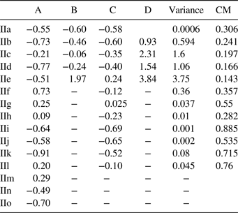
We calculated the five wealth-associated indices for all blocks across all Housepit 54 floors (Supplemental Table 7). We then conducted a PCA (again with IBM SPSS Version 24) that resulted in one significant component capturing 74% of the variance with significant positive loadings on all variables, thus precluding the necessity of rotating the component matrix (Supplemental Tables 8–10). Component scores were generated to assess the contribution of the blocks to the solution, which provides an indicator of relative wealth represented in each occupation area on each floor. Floors IIb–IIe in Block D and Floor IIe in Block B have high positive scores compared to all other blocks on all other floors producing very low positive or negative scores (Table 3). We calculated sample variance for the component scores on all floors with the exception of IIm–IIo to demonstrate which most likely reflect material wealth-based inequality. Sample variance can be impacted by sample size such that all things being equal, larger samples tend to have lower variances. However, our results demonstrate the opposite, with the higher sample size IIa–IIe floors achieving the highest variance scores (Table 3). Thus, these results indicate greatest likely inequality on the IIe floor with continuing recognizable inequality through IIb and a return to greater equality on IIa. Put differently, if the same families occupied the same general spaces across these generations, then we have evidence that one family (Block D group) developed significantly greater material wealth, sources of wealth, and rights to wealth, and succeeded in transmitting it across several generations. The presence of a strong inequality signal on IIb–IIe suggests that it was persistent for about 90 years before a major social shift during IIa and subsequent abandonment. It is interesting in this context that the Block D area registered the highest component scores on wealth measures, but once inequality ended, it was buried by refuse material.
Component Scores and Sample Variance for Wealth Measures for Floors by Excavation Block Areas (A–D) and Cooperation Measure (CM).

Assessing Population and Subsistence Economy on Housepit 54 Floors
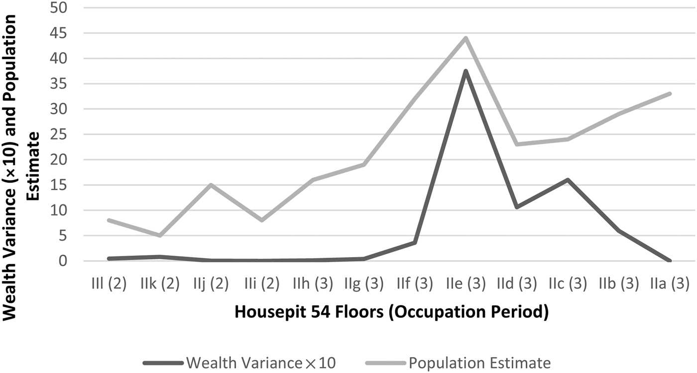
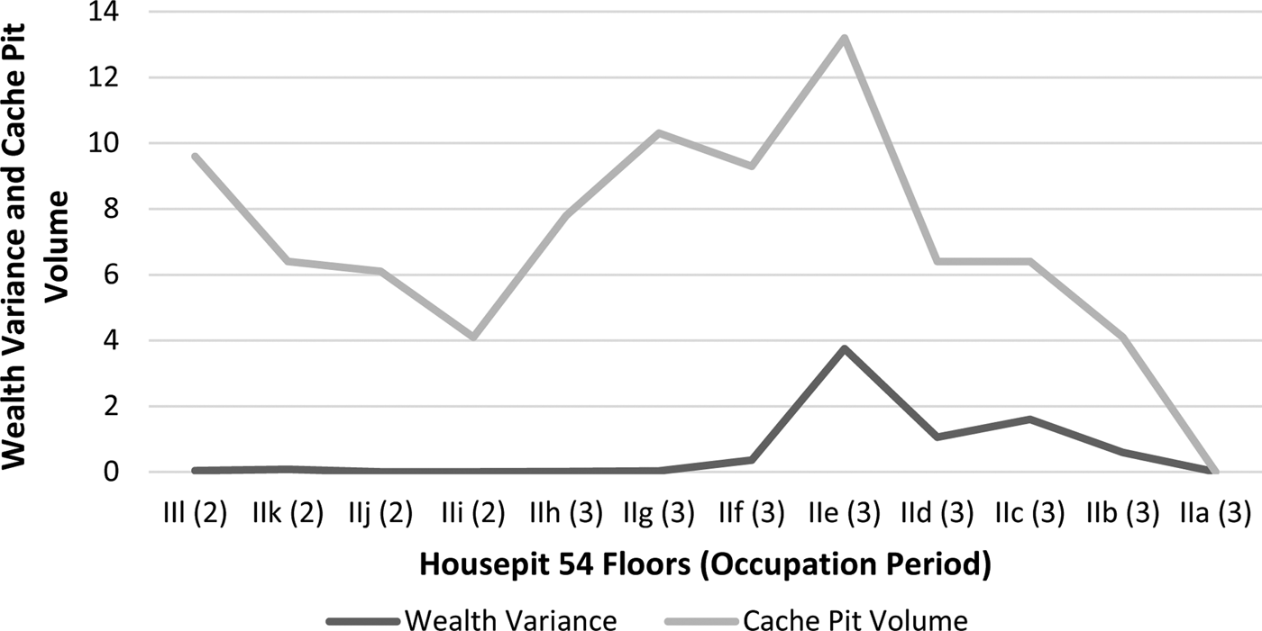
In a previously published study, Prentiss, Foor, and Hampton (Reference Prentiss, Foor and Hampton2018) used fire-cracked rock density to project variation in house populations across the 15 floors. Prentiss, Foor, and Hampton backed up conclusions drawn from fire-cracked rock densities with evidence from hearth volumes and floor area. Results suggest an initial pattern of generally slow growth, followed by very rapid growth from IIf to IIe, reflecting the same pattern of growth across the entire village in early BR3 times. The house population then appears to plummet (floors IIc and IId), coinciding with the onset of the village-wide Malthusian period. Finally, the house population appears to grow slightly between IIb and IIa before final abandonment. Drawing from the same study (Prentiss, Foor, and Hampton Reference Prentiss, Foor and Hampton2018), we used inter-floor variation in relative cache pit volume as a marker of investment in food storage to reflect the state of the household economy. Cache pit volume is very high during the middle BR2 period floors but drops substantially by late BR2, coinciding with village-wide abandonments. Cache pit investment expands rapidly after the beginning of the BR3 period (starting with the IIh floor) and peaks on IIe before steadily declining prior to house abandonment, thus adhering to expectations of likely dynamics regarding storage behavior during Malthusian cycles (Winterhalder et al. Reference Winterhalder, Puleston and Ross2015). Faunal remains are still under investigation, but preliminary assessment suggests drops in access to major game and fish resources immediately prior to population reductions (IId population decline and post-IIa abandonment; Prentiss, Foor, and Murphy Reference Prentiss, Foor, Murphy, Kohler and Smith2018; Walsh Reference Walsh2015). All things considered, the demographic and subsistence economic history of Housepit 54 appears to parallel very closely the same dynamics recognized on the village scale. Wealth variance correlates significantly with our population proxy (r = 0.678; p = 0.015), the primary distinction between the two being that while population increases somewhat more gradually from IIl to IIe, measurable inequality emerges abruptly (Figure 8). Further, inequality declines on IIb and IIa, while population has a slight increase prior to the abandonment. Wealth variance does not quite achieve a significant correlation with relative cache pit volume (r = 0.505; p = 0.094). This discrepancy is largely due to dramatic fluctuation in the BR2 cache pit scores (IIl–IIh) coming at a time when house floor populations are consistently low (Figure 9). By middle to late BR3 times (IIe–IIa), the trends are very close (r = 0.972; p = 0.006).
Wealth variance versus projected population across Housepit 54 floors.

Wealth variance plotted against cache pit volume for Housepit 54 floors.

Assessing Cooperation on Housepit 54 Floors
We developed a quantitative approach for measuring variability in interfamily cooperation regarding shared labor within Housepit 54. We assumed that with greater rates of interfamily cooperation, we would recognize greater spatial variation in activities within the context of repeated domestic spaces. Under this scenario, we expect select talented producers to have engaged in specific manufacture-related activities with the expectation that products would then be shared equally between house members. In contrast, if cooperation in labor was low, we would expect very little indication of specialist activities. Thus, we would see extreme redundancy between domestic areas across the floor. Testing for these possibilities requires an approach that explores the deeper structure of inter-activity area variation in tool representation. Our consistency analysis of tool assemblages demonstrated substantial redundancy between activity areas. However, there was still about 14% variation as measured by the theta coefficient, and it is that variation we explore with our next procedure. In order to make a maximized assessment of tool assemblage variation, we calculated difference matrices on the component scores from our PCA of tool classes (Supplemental Table 6) for each floor (excluding IIm–IIo). For floors IIf–IIl, we then calculated a coefficient of variation on the differences between component scores for each. Concerning floors IIa–IIe, two coefficients of variation were calculated: one for the difference matrix associated with each component on each floor and the other a summary COV for that floor (Table 3). The two-step calculation was necessary for the latter floors given differences in number of values in the matrices (IIf–IIl = 1; IIe–IIb = 6; IIa = 3).
The distribution of scores for all floors illustrates generally higher scores during the IIf–IIl period, with a rapid drop to IIe and consistently low scores thereafter, although with a slight rise across IIe to IIa (Table 3). It is possible that these results are subtly impacted by slight differences in procedure between the IIa–IIe and the IIf–IIl sets. However, there is good reason to believe that they still reflect an underlying social reality. First, the change in house size from IIf to IIe meant twice as many people and greater spatial segregation between family units. Following Thomas and Mark (Reference Thomas and Mark2013), this may have opened the possibility for diverging social networks and differential cooperation. Second, the size and position of cache pits are potentially informative regarding the possibility of shared storage. Cache pits created and used during occupation of the smaller rectangular house (IIf–IIl) are generally large and positioned prominently within one activity area. At the doubling of house size (floor IIe), cache pits shift from Blocks A and C to Blocks B and D, coincident with the concentration of wealth markers in these areas. A large bowl-shaped hearth in the southwestern portion of Block D raises the possibility of a feasting complex occurring uniquely during this period. By late in the life of the IIe floor, all cache pits were filled with either semi-sterile (few artifacts or faunal remains) clay or kitchen refuse. In addition, at least 50% of them were capped by hearth features. Cache pits placed on IIa–IId floors generally include narrow openings and are placed in inconspicuous locations. Thus, we think it is likely that cooperative house-wide use of singular storage facilities could have shifted to family-specific uses of such features along with alternative approaches to storage during a dramatic transition in the IIe occupation.
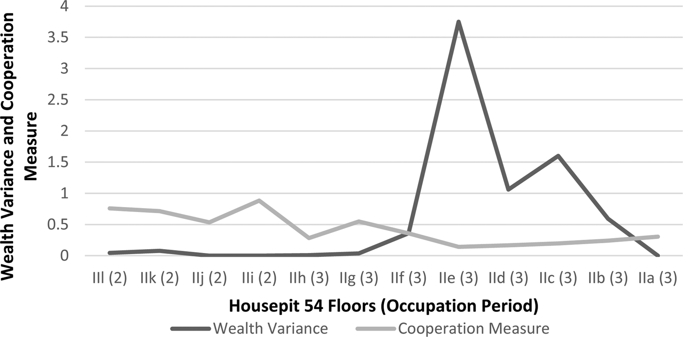
We plotted the wealth variance scores against the cooperation measure; results indicate that wealth-based inequality appeared at the lowest projected point in intra-house cooperation (Figure 10). Wealth variance persists during IIe to IIb but drops to nearly zero on IIa, while the cooperation measure rises to a figure close to some of those predating the IIe floor. The visual pattern is backed by a significant correlation coefficient (r = −0.586; p = 0.045). The cooperation measure is also negatively correlated at a highly significant level with the population proxy (r = −0.807; p = 0.002). To summarize, wealth inequality does correlate positively with population size, and at least for the BR3 period, with the subsistence economy; it appears to occur not because it enhances labor cooperation and property sharing but instead from reduced cooperation in daily work and expanded sense of private (family specific) property.
Plot of cooperation measure versus wealth variance across Housepit 54 floors.

Discussion
This study examined the development of material wealth-based inequality within a single deeply stratified house at the Bridge River site in British Columbia. Housepit 54 was just one house among dozens occupied during BR2 and BR3 times, and its occupants undoubtedly faced their own unique challenges. However, patterning in demographics, household economy, and emergent inequality (including its subsequent decline several generations later) parallels developments we have recognized village-wide (Prentiss, Foor, and Hampton Reference Prentiss, Foor and Hampton2018; Prentiss et al. Reference Prentiss, Lyons, Harris, Burns and Godin2007, Reference Prentiss, Foor, Cross, Harris and Wanzenried2012, Reference Prentiss, Cail and Smith2014). Results strongly indicate that inequality abruptly emerged coincident with the doubling of the house in size under conditions of a population peak during the early-middle BR3 period. It consequently persisted across four floor generations before returning to a strong egalitarian pattern on the final floor prior to abandonment. We argue that material wealth-based inequality, therefore, appears to be linked to a reduction in some forms of intra-house cooperation and comes at the beginning of declining subsistence productivity. Given this scenario, we reject the aggrandizer hypothesis.
The scalar stress hypothesis provides a partial fit, although our results illustrate some nuance requiring further consideration. Our data raise the possibility that at peak population, the community hit a socioecological tipping point that encouraged a shift in permitted behavior with regard to variation in access to material wealth (cf. Dunbar Reference Dunbar1993; Fitzhugh Reference Fitzhugh2003). This probably required new forms of sociopolitical cooperation, although it is not strongly evident in our data with the exception of the possible short-lived feasting complex on the IIe floor in Housepit 54. Change in the nature of cooperation did not stave off village fissioning. Significant village-wide population reduction began immediately following the population peak; it is possible that the rapid early BR3 population expansion simply overshot the ability of the community to socially compensate for the sudden demands on resources. Thus, the Malthusian ceiling hypothesis remains highly relevant to our understanding of emergent inequality.
Our data from Housepit 54 also illustrate an apparent return to intra-house sharing of labor and goods after several generations, characterized by material wealth-based inequality. This pattern offers implications for how we understand the wider Mid-Fraser abandonment process (cf. Hayden and Ryder Reference Hayden and Ryder1991; Kuijt Reference Kuijt2001). The abandonment of Housepit 54 during and after the occupation of the IIa floor was accompanied by what appears to have been a closing of the Block D floor area during the life of IIa and then a large-scale burning and collapsing of the associated stratum Va roof. The latter occurred on a scale not recognized for any previous Housepit 54 floors. This seems to imply that the abandonment process had as much to do with reorganizing a social order as escaping a difficult socioeconomic situation. In turn, this suggests that Mid-Fraser folk sought to return to a more ancient and well-favored pattern of relative economic and political egalitarianism during the terminal BR3 period and likely for centuries thereafter.
Acknowledgments
The Bridge River Archaeological Project is a collaborative partnership between the University of Montana and Xwísten, the Bridge River Indian Band. Susan James, Bradley Jack, and Gerald Michel played significant roles in facilitating the Housepit 54 project (including providing the permit to conduct the field and lab research). Many Band members participated in the fieldwork. The 2012–2016 field seasons at Housepit 54 were supported by two grants from the National Endowment for the Humanities (Grants RZ-51287–11 and RZ-230366–1). Any views, findings, conclusions, or recommendations expressed in this article do not necessarily represent those of the National Endowment for the Humanities. The 2008 field season at Bridge River that included initial excavations of Housepit 54 was funded by a grant from the National Science Foundation (BCS-0713013). We thank students and volunteers from the University of Montana, Simon Fraser University, Hamilton College, University of Michigan, and University of Notre Dame who participated in the Housepit 54 project. Kaitlin Pipitone translated our Spanish abstract. We thank six anonymous peer reviewers for their insightful comments. We also thank Lynn Gamble and staff for moving the manuscript through the editorial process. Prentiss thanks the University of Montana for sabbatical time and travel funding and the McDonald Institute for Archaeological Research at the University of Cambridge for providing a visiting scholar position. None of the authors have financial interests and/or affiliations with institutions, organizations, and companies relevant to this submission, or those of anyone with whom any of us directly share income (e.g., spouse, minor child, or business partner) or of any other third party whose interests may affect our decision-making (e.g., sibling or adult child).
Data Availability Statement
Raw data used to develop the analyses in this paper are provided in the tables and supplemental tables within this article.
Supplemental Materials
For supplementary material accompanying this paper, visit https://doi.org/10.1017/aaq.2018.56.
Supplemental Figure 1. Plan views of floors IIm–IIo illustrating positions of hearths, cache pits, and large rocks.
Supplemental Figure 2. Plan views of floors IIl–IIf illustrating positions of hearths, cache pits, and large rocks.
Supplemental Figure 3. Plan views of floors IIe–IIa illustrating positions of hearths, cache pits, and large rocks.
Supplemental Table 1. Lithic Tool Data from Housepit 54 Floors.
Supplemental Table 2. Correlation Matrix for Principal Components Analysis (PCA) on Lithic Tools from Housepit 54 (providing the statistical foundation for development of the PCA illustrated in Supplemental Tables 3–5).
Supplemental Table 3. Statistics for PCA on Lithic Tools from Housepit 54.
Supplemental Table 4. Unrotated Component Matrix for PCA on Lithic Tools from Housepit 54.
Supplemental Table 5. Rotated Component Matrix from PCA on Lithic Tools from Housepit 54.
Supplemental Table 6. Component Scores from PCA on Lithic Tools from Housepit 54.
Supplemental Table 7. Wealth Measures for Housepit 54 Floor Strata by Block Areas.
Supplemental Table 8. Correlation Matrix for PCA of Wealth Measures.
Supplemental Table 9. Statistics for PCA of Wealth Markers.
Supplemental Table 10. Component Matrix for PCA of Wealth Markers.