1. Introduction
The study of fluid flows in Hele-Shaw cells (i.e. the thin gap between two rigid plates) is of great interest, both for direct applications in, e.g., industrial systems and microfluidic devices, and due to the mathematical similarities to fluid flow in porous media, with applications to, e.g., oil recovery from porous rock deep underground. In many cases, there is more than one fluid involved, e.g. when a Hele-Shaw cell is being emptied.
A basic well-studied case is the motion of a bubble of gas in a Hele-Shaw cell filled with viscous liquid. When the gap height
 $h$
of the cell is small compared with the extent of the bubble, the flow can be modelled with quantities averaged across the gap. Away from the bubble, the lubrication equations for the viscous liquid yield a flux proportional to the pressure gradient with proportionality coefficient
 $h^{3}/12{\it\mu}$
, where
 ${\it\mu}$
is the dynamic viscosity of the liquid. The gas bubble may be in contact with the walls of the cell, or it may be bounded by thin films of liquid wetting the walls. In either case, the pressure in the inviscid bubble is constant. Near the bubble tip, the flow field is more complicated, but its details are usually ignored and effective matching conditions are applied between the liquid and bubble regions (e.g. Park & Homsy Reference Park and Homsy1984).
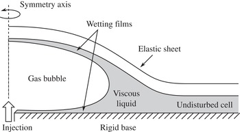
Where the bubble front advances, the gas–liquid interface may be susceptible to the Saffman–Taylor viscous-fingering instability, which is driven by the viscosity difference between the two phases but is resisted by the surface tension acting on the interface (e.g. Homsy Reference Homsy1987). However, recent experiments (Pihler-Puzović et al. Reference Pihler-Puzović, Illien, Heil and Juel2012) and numerical simulations (Pihler-Puzović et al. Reference Pihler-Puzović, Périllat, Russell, Juel and Heil2013; Pihler-Puzović, Juel & Heil Reference Pihler-Puzović, Juel and Heil2014) have found that the onset of the viscous-fingering instability is delayed if the upper rigid wall of the horizontal Hele-Shaw cell is replaced with an elastic sheet (figure 1). The injected gas deflects the sheet upwards, altering the geometry of the cell and hence the stability properties. These studies focused primarily on the instability, and hence did not attempt to give a detailed theoretical description of the unperturbed axisymmetric base flow. The main focus of the present paper is to obtain a complete theoretical understanding of this base flow, i.e. the two-phase spreading of a gas bubble in an elastic-walled Hele-Shaw cell filled with viscous liquid. In particular, we examine the effects of the capillary meniscus at the bubble tip and the wedge of liquid that accumulates ahead of it. (A related system with a different geometry where a bubble advances in an elastic tube was proposed by Gaver, Samsel & Solway (Reference Gaver, Samsel and Solway1990) as a simple model for airway reopening and has been studied extensively – see, e.g., Heil & Hazel (Reference Heil and Hazel2011) for a review.)
Schematic figure of the two-phase system, where gas is injected and spreads radially in an elastic-walled Hele-Shaw cell.

In Part 1 of this work (Pihler-Puzović et al. Reference Pihler-Puzović, Juel, Peng, Lister and Heil2015), we presented a model for the physical system that couples the Föppl–von-Kármán equations for the elastic sheet to the Navier–Stokes equations for the viscous liquid and includes a free surface that corresponds to the gas–liquid interface. The governing equations were solved numerically using the finite-element library oomph-lib (Heil & Hazel Reference Heil, Hazel, Schäfer and Bungartz2006). The time evolution of both the bubble radius and the height profile was also measured in experiments, and excellent agreement was obtained between the theoretical model and the experiments.
Since the full Navier–Stokes equations are computationally expensive to solve and difficult to analyse, it is desirable to exploit the large aspect ratio of the cell to obtain simplified governing equations for the liquid using the lubrication approximation. Previous lubrication models (Al-Housseiny, Christov & Stone Reference Al-Housseiny, Christov and Stone2013; Pihler-Puzović et al. Reference Pihler-Puzović, Périllat, Russell, Juel and Heil2013) have neglected the films of wetting fluid left behind the bubble tip. In Part 1, we showed that such a lubrication model noticeably (but not catastrophically) underestimates the bubble radius compared with the experimental and Navier–Stokes results.
In the first part of this paper, we begin by deriving an improved lubrication model which includes the effects of the wetting films. Parametrization of the flow near the meniscus using asymptotic results by Park & Homsy (Reference Park and Homsy1984) augmented by numerical results by Reinelt & Saffman (Reference Reinelt and Saffman1985) yields two effective boundary conditions: a kinematic condition for the liquid velocity at the meniscus, which includes corrections for the amount of liquid left behind in the wetting films, and a dynamic condition for the pressure drop across the meniscus, which is due to both capillary and viscous effects. We validate our model against the Navier–Stokes model from Part 1 and show an excellent agreement between the two.
In the second part of this paper, we proceed to investigate the behaviour of the two-phase system using asymptotic analysis of the lubrication model. We focus on times when a sufficient amount of gas has been injected that the deflection of the sheet by the bubble is much larger than the undisturbed cell height
 $h_{0}$
. The bubble spreads radially outwards and displaces the viscous liquid that initially filled the cell, which accumulates in a wedge ahead of the bubble tip. The spreading rate of the bubble is given by the speed at which the elastic sheet ‘peels away’ from the rigid base at the tip of the advancing liquid wedge, and depends on the interplay between elastic, viscous and capillary forces in and around the wedge.
A simpler physical system (also studied in Part 1) is the single-phase analogue, where the injected fluid is the same as the viscous liquid that initially fills the cell, and no interface with capillary effects is present. This case has been analysed recently by Lister, Peng & Neufeld (Reference Lister, Peng and Neufeld2013) and Hewitt, Balmforth & De Bruyn (Reference Hewitt, Balmforth and De Bruyn2014) (while similar problems have been treated by King & Bowen (Reference King and Bowen2001) and Flitton & King (Reference Flitton and King2004)). These studies investigated the spreading of the liquid driven by various combinations of elastic bending and tension forces (in the sheet) and gravitational forces (acting on the liquid), again under the assumption that a large amount of extra fluid has been injected, deflecting the elastic sheet upwards by a large amount to form a blister.
The radius
 $R(t)$
of the blister of injected fluid increases with time as the fluid spreads beneath the elastic sheet. Since the blister height is much larger than
 $h_{0}$
, the pressure variation in the bulk of the blister due to the viscous flow is asymptotically small (although the first-order corrections can be quite large in the tension-dominated case). At the edge of the blister, where the cell height decreases towards
 $h_{0}$
, the viscous effects become noticeable and control the rate
 ${\dot{R}}$
at which the blister advances due to the sheet peeling away from the base. Here, the system takes the form of a travelling wave, moving outwards with velocity
 ${\dot{R}}$
.
If either bending or tension forces dominate at the blister edge, then the peeling speed depends on either the apparent curvature
 ${\it\kappa}_{b}$
or the apparent slope
 ${\it\alpha}_{b}$
respectively at the blister edge, according to the peeling laws
 $$\begin{eqnarray}{\dot{R}}=0.472\frac{Bh_{0}^{1/2}{\it\kappa}_{b}^{5/2}}{12{\it\mu}}\quad \text{ or }\quad {\dot{R}}=\frac{T{\it\alpha}_{b}^{3}}{36{\it\mu}\ln {\it\Delta}},\end{eqnarray}$$
where
 $B$
and
 $T$
are the bending stiffness of the sheet and the elastic tension in the sheet, and
 ${\it\Delta}$
is the ratio between the blister and peeling length scales. Following Lister et al. (Reference Lister, Peng and Neufeld2013), we refer to these laws as peeling by bending and peeling by pulling. We note that peeling by pulling is analogous to the spreading of a capillary droplet (e.g. Bonn et al.
Reference Bonn, Eggers, Indekeu, Meunier and Rolley2009) with surface tension replaced by elastic tension, and that the corresponding law (1.1b
) is the elastic analogue of the Cox–Voinov law (Voinov Reference Voinov1976; Cox Reference Cox1986).
For the two-phase case where gas is injected, there are two main differences. First, the gas provides no viscous resistance to the spreading of the blister. This has only a minor effect on the analysis, since in the single-phase case the viscous pressure drop in the bulk of the blister is small. Second, there is a gas–liquid interface on which surface tension can act. In particular, the capillary pressure drop across the meniscus at the bubble tip lowers the pressure in the liquid wedge and hence sucks down the elastic sheet. The main aim of this paper is to investigate this effect and obtain two-phase peeling-by-bending and peeling-by-pulling laws analogous to the single-phase results (1.1).
In the course of the analysis, we will identify three key transition times
 $t_{0}$
,
 $t_{1}$
,
 $t_{2}$
between different asymptotic behaviours. We pass over the ‘early’ times (
 $t\ll t_{0}$
) when the deflection of the sheet is small and focus on times
 $t\gg t_{0}$
when the deflection is large. At ‘moderate’ times (
 $t_{0}\ll t\ll t_{1}$
), viscous effects dominate and capillary effects are negligible. Hence, as was argued by Lister et al. (Reference Lister, Peng and Neufeld2013), the single-phase analysis applies also to the two-phase case. As time passes, the capillary effects grow in importance, and they dominate the viscous effects at ‘late’ times (
 $t_{1}\ll t\ll t_{2}$
). At ‘very late’ times (
 $t\gg t_{2}$
), capillary forces remain dominant but the structure of the solution ahead of the peeling region changes.
This paper is laid out as follows. We present the governing equations for our improved lubrication model in § 2, and validate them by comparing their solutions with the numerical and experimental results from Part 1 in § 3. The numerical results are used to motivate the asymptotic analysis, which is performed in two parts: we investigate moderate and late times (
 $t_{0}\ll t\ll t_{2}$
) in § 4 and very late times (
 $t\gg t_{2}$
) in § 5. The results are summarized in § 6.
2. Governing equations – lubrication model with a meniscus
We consider axisymmetric spreading of a viscous liquid on a horizontal rigid surface under an elastic sheet due to the injection of inviscid gas (figure 1). The viscosity of the liquid is
 ${\it\mu}$
and the surface tension at the gas–liquid interface is
 ${\it\gamma}$
. The thin overlying elastic sheet is assumed to be a linearly elastic solid with Young’s modulus
 $E$
, Poisson’s ratio
 ${\it\nu}$
and thickness
 $d$
, so that its bending stiffness is
 $B=Ed^{3}/12(1-{\it\nu}^{2})$
.
The system is assumed to have much greater horizontal length scales than height scales (except near the bubble tip), so that we can employ vertically integrated/averaged quantities which are functions of a horizontal position vector
 $\boldsymbol{x}=r\boldsymbol{e}_{r}$
(where
 $r$
is the radial coordinate and
 $\boldsymbol{e}_{r}$
is the radial unit vector) and time
 $t$
. We use primes and overdots to denote differentiation with respect to
 $r$
and
 $t$
respectively, and also make use of the horizontal gradient operator
 $\boldsymbol{{\rm\nabla}}$
for expressions such as
 $\boldsymbol{{\rm\nabla}}\boldsymbol{\cdot }(f\boldsymbol{e}_{r})=(1/r)(rf)^{\prime }$
. We seek to predict the gas-bubble radius
 $R(t)$
(i.e. the distance from the injection point to the bubble tip) and the cell height profile
 $h(r,t)$
. The effective fluid pressure
 $p(r,t)$
(from which atmospheric pressure is subtracted), horizontal liquid velocity
 $\boldsymbol{u}=u(r,t)\boldsymbol{e}_{r}$
and flux
 $\boldsymbol{q}=q(r,t)\boldsymbol{e}_{r}$
, and the radial tension
 $T(r,t)$
in the sheet (integrated across the thickness of the sheet) will be also be used in the analysis.
For simplicity, we neglect any gravitational (i.e. hydrostatic) effects. As Lister et al. (Reference Lister, Peng and Neufeld2013) and Hewitt et al. (Reference Hewitt, Balmforth and De Bruyn2014) have shown, this is appropriate when the horizontal length scales of any liquid region are small compared with a bending–gravity or tension–gravity length scale. Moreover, this approximation was seen to be adequate for the two-phase experiments in Part 1. We also neglect any direct surface-tension forces on the sheet if there is a dewetting contact line, and the small capillary pressure drop across the gas–liquid interface above and below the bubble if thin wetting films are deposited on the elastic sheet. The analysis in § 4 confirms that these effects are indeed small. Hence, the only surface-tension effects considered are those on the highly curved meniscus at the bubble tip.
2.1. Model for the elastic sheet
We assume that the inertia and shear stresses on the sheet are both negligible, so that it can be modelled using the Föppl–von-Kármán equations (see, e.g., Audoly & Pomeau (Reference Audoly and Pomeau2010) for a detailed treatment). These equations describe the elastic response of the sheet due to bending forces as well as tension forces, which were seen in Part 1 to be important. Tension is induced by the deflection of the sheet, even in the absence of externally applied tension, and its value is found by solving the second Föppl–von-Kármán equation, which describes the force balance in the direction tangent to the sheet, together with the condition for compatibility of strains. In an axisymmetric geometry, the resultant equation takes the simple form (Lister et al. Reference Lister, Peng and Neufeld2013)
 $$\begin{eqnarray}\frac{1}{r}(r^{3}T^{\prime })^{\prime }=-\frac{Ed}{2}h^{\prime 2}.\end{eqnarray}$$
The first Föppl–von-Kármán equation, which describes the force balance in the direction normal to the sheet, yields the coupling between the (effective) fluid pressure
 $p$
and the deflection
 $h-h_{0}$
, and can be written as
 $$\begin{eqnarray}p=B{\rm\nabla}^{4}h-\boldsymbol{{\rm\nabla}}\boldsymbol{\cdot }(T\boldsymbol{{\rm\nabla}}h).\end{eqnarray}$$
The two terms describe bending and tension effects respectively, and a scaling analysis reveals that effects due to deflection-induced tension are important when the deflection
 $h-h_{0}$
is large compared with the sheet thickness
 $d$
; see Part 1. The radial tension
 $T$
is related to the Airy stress function
 ${\it\phi}$
from Part 1 via
 $rT=\text{d}{\it\phi}^{\prime }$
.
2.2. Model for the fluids
Near the meniscus at the bubble tip
 $r=R(t)$
, the flow in the cell can be quite complicated, with comparable length scales in the radial and vertical directions. Away from the meniscus, however, the radial scales are much longer. Hence, we model only the regions ahead of and behind the meniscus in detail, while treating the meniscus region as a sharp interface at
 $R(t)$
, with approximate interfacial conditions to be determined.
In the ‘liquid region’
 $r>R(t)$
, the cell is filled with viscous liquid which obeys the lubrication equations. If the radial motion of the overlying sheet is neglected, then the flow profile is parabolic, driven by the effective pressure
 $p$
, and we obtain
 $$\begin{eqnarray}\boldsymbol{q}=h\boldsymbol{u}=-\frac{h^{3}}{12{\it\mu}}\boldsymbol{{\rm\nabla}}p,\quad {\dot{h}}=-\boldsymbol{{\rm\nabla}}\boldsymbol{\cdot }\boldsymbol{q}=\boldsymbol{{\rm\nabla}}\boldsymbol{\cdot }\left(\frac{h^{3}}{12{\it\mu}}\boldsymbol{{\rm\nabla}}p\right)\quad \text{in }r>R(t).\end{eqnarray}$$
In the ‘bubble region’
 $r<R(t)$
, the cell contains a bubble of inviscid gas at some constant pressure
 $p_{b}(t)$
(above atmospheric pressure). Having neglected the effects of any wetting films of liquid on the top and bottom walls in this region, we obtain
 $$\begin{eqnarray}p=p_{b}(t)\quad \text{ in }r<R(t).\end{eqnarray}$$
If the gas is injected at a prescribed flow rate, as in the experiments of Part 1, then
 $p_{b}(t)$
is unknown and must be determined from conservation of gas volume; see (2.13) below.
2.3. Model for the capillary meniscus
We seek effective interfacial conditions describing the behaviour of the flow near the meniscus at
 $R(t)$
. As the slope of the elastic sheet is small and its vertical velocity is much smaller than the horizontal fluid velocities, the tip of the bubble behaves as if it were advancing steadily in a parallel-walled Hele-Shaw cell with fixed gap height. We use results for this simpler case, which depend on the instantaneous capillary number
 $\mathit{Ca}={\it\mu}{\dot{R}}(t)/{\it\gamma}$
, as approximations for the more complicated system.
We note first that the curved meniscus introduces a discontinuity in the pressure
 $p$
across the interface, but we neglect any direct effects on the elastic sheet (such as the point load from the meniscus at the contact line if there is dewetting). Since
 $p$
is coupled to
 $h^{\prime \prime \prime \prime }$
(and possibly lower derivatives) by (2.2), this yields the condition
 $$\begin{eqnarray}h,~h^{\prime },~h^{\prime \prime },~h^{\prime \prime \prime }\text{continuous across }r=R(t).\end{eqnarray}$$
2.3.1. Without wetting films
If no wetting films of liquid are left behind the meniscus, then conservation of liquid volume yields a kinematic condition for the (depth-averaged) horizontal liquid velocity,
 $$\begin{eqnarray}u(R^{+})={\dot{R}}.\end{eqnarray}$$
We take the vertical profile of the meniscus to be an arc of a circle which contacts the (parallel) cell walls at a zero contact angle, so its vertical curvature is
 $2/h$
. The horizontal curvature of the meniscus is small compared with its vertical curvature, so we neglect it here. Hence, the pressure drop, given by the Young–Laplace equation, is
 $$\begin{eqnarray}[p]_{-}^{+}=-\frac{2{\it\gamma}}{h}\quad \text{at }r=R(t).\end{eqnarray}$$
2.3.2. With wetting films
When wetting films are left behind the meniscus, their thickness is determined by the dynamics in the meniscus region and depends on the capillary number
 $\mathit{Ca}$
. For a two-dimensional bubble advancing in a rigid parallel-walled Hele-Shaw cell with gap height
 $h$
, we let
 $h\,f_{1}(\mathit{Ca})$
denote the total thickness of the deposited films and
 $(2{\it\gamma}/h)\,f_{2}(\mathit{Ca})$
denote the pressure drop across the meniscus region due to viscous and capillary effects. Based on the work of Bretherton (Reference Bretherton1961), Park & Homsy (Reference Park and Homsy1984) calculated the asymptotic results
 $$\begin{eqnarray}f_{1}(\mathit{Ca})\sim 1.34\,\mathit{Ca}^{2/3},\quad f_{2}(\mathit{Ca})\sim 1+3.80\,\mathit{Ca}^{2/3}\quad \text{as }\mathit{Ca}\rightarrow 0.\end{eqnarray}$$
For our numerical calculations, where
 $\mathit{Ca}$
is too large at early times for these asymptotic results to apply, we turn to numerical results given in figures 4 and 5 of Reinelt & Saffman (Reference Reinelt and Saffman1985). These results agree with (2.7) in the small-
 $\mathit{Ca}$
limit, and have the large-
 $\mathit{Ca}$
behaviour that
 $f_{1}$
tends to a constant while
 $f_{2}$
becomes proportional to
 $\mathit{Ca}$
(indicating that the pressure jump has a viscous scaling
 ${\it\mu}{\dot{R}}/h$
independent of
 ${\it\gamma}$
). We extracted data points from the figures and performed a numerical fit to simple functional forms with appropriate asymptotic behaviours, resulting in the following expressions:
 $$\begin{eqnarray}f_{1}(\mathit{Ca})=\frac{\mathit{Ca}^{2/3}}{0.76+2.16\mathit{Ca}^{2/3}},\quad f_{2}(\mathit{Ca})=1+\frac{\mathit{Ca}^{2/3}}{0.26+1.48\mathit{Ca}^{2/3}}+1.59\mathit{Ca}.\end{eqnarray}$$
(A similar approach was used by Jensen et al. (Reference Jensen, Horsburgh, Halpern and Gaver2002) in their study of airway reopening, but their formulae for
 $f_{1}$
and
 $f_{2}$
were chosen for accuracy at intermediate values of
 $\mathit{Ca}$
and agreement with (2.7) was not enforced.)
For the bubble in the elastic cell, we assume that
 $f_{1}$
and
 $f_{2}$
can be used at every instant in time to describe the amount of liquid being deposited behind the advancing bubble and the effective pressure drop across the meniscus region. Hence, we obtain the modified kinematic and dynamic boundary conditions
 $$\begin{eqnarray}u(R^{+})={\dot{R}}[1-f_{1}({\it\mu}{\dot{R}}/{\it\gamma})],\quad [p]_{-}^{+}=-\frac{2{\it\gamma}f_{2}({\it\mu}{\dot{R}}/{\it\gamma})}{h}\quad \text{at }r=R(t).\end{eqnarray}$$
Equations (2.8) describe how the interfacial velocity
 ${\dot{R}}$
is larger than the depth-averaged liquid velocity
 $u(R^{+})$
due to some of the liquid being left behind on the cell walls, and how the interfacial pressure drop is increased due to the viscous and capillary effects near the meniscus. They constitute our ‘improved’ meniscus model, as compared with the ‘simple’ model (2.6). These models provide the appropriate connection between the lubrication equation (2.3) for the liquid region and the constant-pressure condition (2.4) for the bubble region.
2.4. Initial and boundary conditions
In order to complete the model, we need to prescribe initial and boundary conditions. Due to axisymmetry, we have
 $$\begin{eqnarray}h^{\prime }=h^{\prime \prime \prime }=0,\quad T^{\prime }=0\quad \text{at }r=0.\end{eqnarray}$$
In the idealized case of an infinite Hele-Shaw cell (
 $R_{cell}=\infty$
), it is natural to assume that the sheet is undisturbed with no tension far ahead of the bubble,
 $$\begin{eqnarray}h\rightarrow h_{0},\quad p\rightarrow 0,\quad T\rightarrow 0\quad \text{as }r\rightarrow \infty .\end{eqnarray}$$
For direct comparisons with results from Part 1, however, we must model an axisymmetric Hele-Shaw cell with finite radius
 $R_{cell}$
. As disturbances to
 $h$
typically decay exponentially on a short length scale (Lister et al.
Reference Lister, Peng and Neufeld2013), the system is quite insensitive to the exact form of the outer boundary conditions for
 $h$
until the spreading is very close to the edge of the cell. Thus, for simplicity, we apply ‘clamped’ conditions with no flux,
 $$\begin{eqnarray}h=h_{0},\quad h^{\prime }=0,\quad p^{\prime }=0\quad \text{at }r=R_{cell}.\end{eqnarray}$$
One must be slightly more careful with the boundary conditions for tension, as it only decays algebraically (the generic far-field behaviour is
 $T\sim A+B/r^{2}$
for arbitrary constants
 $A$
,
 $B$
). We approximate the sheet as a circular disc whose edge is free to move horizontally and is not under any applied tension,
 $$\begin{eqnarray}T=0\quad \text{at }r=R_{cell}.\end{eqnarray}$$
Following Part 1, we assume that initially the sheet is flat and the gas bubble has a given radius,
 $$\begin{eqnarray}h=h_{0},\quad R=R_{0}\quad \text{at }t=0.\end{eqnarray}$$
Gas is then injected at a constant volume flux
 $\dot{V}$
, and the injected volume
 $\dot{V}t$
of gas determines the bubble pressure
 $p_{b}(t)$
. When films of liquid are left behind in the bubble region, it is unnecessarily complicated to keep track of the actual volume of gas. Instead, we (equivalently) prescribe the total amount of excess fluid (gas and liquid) in the cell, which does not require keeping track of the liquid film thickness. This yields
 $$\begin{eqnarray}\int _{0}^{R_{cell}}(h(r,t)-h_{0})\,2{\rm\pi}r\,\text{d}r=\dot{V}t.\end{eqnarray}$$
3. Numerical results with the improved meniscus model
We have developed an implicit finite-difference numerical method to calculate solutions to the governing equations presented in § 2. We first validate the meniscus model by comparing our results with numerical solutions of the full Navier–Stokes equations. These reference results were calculated in Part 1, where they were shown to agree quantitatively with experimental data. We then examine the numerical results for later times, discovering new regimes beyond those covered by Part 1. These results are used to inform our asymptotic analyses in §§ 4 and 5.
3.1. Direct comparison with results from Part 1
We start by examining numerical results obtained using parameter values corresponding to the experiments with latex sheets in Part 1 (
 $E=2.1$
MPa,
 $d=0.34$
mm,
 ${\it\mu}=0.9624$
Pa s,
 ${\it\gamma}=0.021$
N m
 $^{-1}$
,
 $h_{0}=0.56$
mm). We compare the Navier–Stokes results, lubrication results with no wetting films (2.6) and lubrication results with wetting films described by the meniscus model (2.8).
Comparison of instantaneous height and pressure profiles at
 $t=10$
s (latex sheet, injection flux
 $\dot{V}=150$
ml min
 $^{-1}$
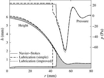
) for three solutions: the full Navier–Stokes equations from Part 1 (also showing the gas–liquid interface, with the liquid shaded), the simple lubrication model (also showing the meniscus position) and the improved lubrication model (also showing the meniscus position and the thin films left behind) (cf. figures 6 and 8 of Part 1).

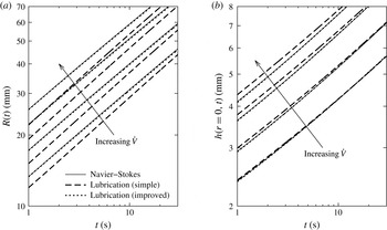
Figure 2 shows a typical example of instantaneous height and pressure profiles. As was noted in Part 1, the lubrication model without wetting films underestimates the meniscus position, while the predicted height profile is relatively accurate. The improved model shows excellent agreement in terms of both the meniscus position and the height profile. Figure 3 shows the time evolution of the bubble radius and the central cell height and confirms these findings for a wide range of parameters.
For the improved model (dotted lines in figure 2), the lines shown inside the height profile indicate the thickness of the films deposited by the passing meniscus, neglecting any subsequent motion of the fluid (i.e. assuming that the deposited films are static). As such, they only provide an estimate of the film thicknesses that are found by the full Navier–Stokes calculation, but nevertheless show very good agreement with the numerics from Part 1. (The region near the origin with no films is the initial position of the bubble in our calculation.)
Comparison of the time evolution of the bubble radius
 $R(t)$
and the central cell height
 $h(r=0,t)$
(with injection flux
 $\dot{V}=50,~100,~200,~300$
ml min
 $^{-1}$
) for three solutions: the full Navier–Stokes equations from Part 1, the simple lubrication model and the improved lubrication model (cf. figures 9 and 10 of Part 1).

We conclude that the improved model, with the interfacial conditions (2.8), provides an excellent approximation to the Navier–Stokes model and hence, by extension, the physical system. This also confirms that the main shortcoming of the simple lubrication model, with interfacial conditions (2.6), and the cause of its mismatch with the Navier–Stokes and experimental results, is indeed the lack of accurate modelling of the meniscus, as was stated in Part 1.
3.2. Preliminary numerical study to inform the asymptotic analysis
In order to investigate the physical effects behind the behaviour observed in § 3.1 and Part 1, we will perform an asymptotic analysis of the generic peeling problem in §§ 4 and 5. Here, we perform a preliminary numerical study in order to guide this asymptotic analysis.
3.2.1. Bending- and tension-dominated cases
First, we investigate the relative importance of bending and tension forces in the elastic response of the overlying sheet, i.e. the relative strengths of the bending term
 $p_{B}=B{\rm\nabla}^{4}h$
and the tension term
 $p_{T}=-\boldsymbol{{\rm\nabla}}\boldsymbol{\cdot }(T\boldsymbol{{\rm\nabla}}h)$
in (2.2). From (2.2), we identify a bending–tension length scale
 $L_{BT}=\sqrt{B/T}$
(which, like the tension
 $T(r,t)$
, varies with time and position). If the horizontal length scales of the system are much shorter than
 $L_{BT}$
, then bending forces dominate (
 $p\approx p_{B}\gg p_{T}$
). If the horizontal length scales are much longer than
 $L_{BT}$
, then tension forces dominate (
 $p\approx p_{T}\gg p_{B}$
).
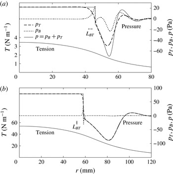
Figure 4(a) shows a representative pressure profile
 $p=p_{B}+p_{T}$
alongside the individual contributions
 $p_{B}$
and
 $p_{T}$
(again using the latex sheet parameter values). We note that the tension
 $T$
does vary with position, but remains at the same scale throughout the regions of interest, so the value of
 $L_{BT}$
calculated using
 $T$
evaluated at the interface is representative. The bubble radius is much larger than
 $L_{BT}$
, and consequently the bubble region is tension-dominated. In the peeling wave ahead of the gas–liquid interface, the horizontal length scale is comparable with
 $L_{BT}$
, and consequently both bending and tension forces are important. Figure 4(b) shows results using parameter values (
 $E=3.7$
GPa,
 $d=0.030$
mm,
 ${\it\mu}=0.305$
Pa s,
 ${\it\gamma}=0.065$
N m
 $^{-1}$
,
 $h_{0}=0.56$
mm) corresponding to the experiments in Part 1 with polypropylene sheets. For these much thinner sheets,
 $L_{BT}$
is much smaller and consequently tension forces dominate everywhere (except in a small region of length
 $L_{BT}$
near the interface, which can be neglected).
Profiles of tension
 $T$
and pressure (bending pressure
 $p_{B}=B{\rm\nabla}^{4}h$
, tension pressure
 $p_{T}=-\boldsymbol{{\rm\nabla}}\boldsymbol{\cdot }(T\boldsymbol{{\rm\nabla}}h)$
and total pressure
 $p$
) at time
 $t=10$
s for the lubrication calculation with the improved meniscus model. The parameters are taken from the experiments of Part 1 with injection flux
 $\dot{V}=150$
ml min
 $^{-1}$
and (a) latex or (b) polypropylene sheets. The bending–tension length scale
 $L_{BT}=\sqrt{B/T}$
is calculated using the value of the tension at the interface and shown using horizontal bars ((a)
 $L_{BT}=2.0$
mm, (b)
 $L_{BT}=0.52$
mm).

For our asymptotic analyses in §§ 4 and 5, we assume that the Hele-Shaw cell is infinite (
 $R_{cell}=\infty$
) and also restrict ourselves to two idealized cases for simplicity: (i) the bending-dominated case, when tension forces can be neglected everywhere (
 $p=p_{B}$
,
 $T=0$
), and (ii) the tension-dominated case, when bending forces can be neglected everywhere (
 $p=p_{T}$
,
 $B=0$
). Although the bending-dominated case is not directly relevant to the experiments in Part 1, it is simpler to analyse and will be shown in §§ 4 and 5 to exhibit the same qualitative features as the more complicated tension-dominated case. Thus, it serves as a good starting point for our analysis. Moreover, Lister et al. (Reference Lister, Peng and Neufeld2013) showed that the bending-dominated case is readily achieved in experiments where the sheet thickness
 $d$
is much larger than the initial cell height
 $h_{0}$
. The tension-dominated case, however, is directly applicable to the polypropylene experiments. The latex experiments do not fall into either limiting case as both
 $p_{T}$
and
 $p_{B}$
are significant in the wedge region ahead of the interface (figure 4
a).
In the numerical calculations for the tension- and bending-dominated cases, we employ non-dimensionalizations using the viscous scales
 $$\begin{eqnarray}\displaystyle & \text{bending: } & \displaystyle \text{height }h_{0},\quad \displaystyle \text{length }L_{0}=\left(\frac{Bh_{0}^{4}}{12{\it\mu}\dot{V}}\right)^{1/4},\quad \text{time }t_{0}=\frac{h_{0}L_{0}^{2}}{\dot{V}};\end{eqnarray}$$
 $$\begin{eqnarray}\displaystyle & \text{tension: } & \displaystyle \text{height }h_{0},\quad \displaystyle \text{length }L_{0}=\left(\frac{Edh_{0}^{6}}{12{\it\mu}\dot{V}}\right)^{1/4},\quad \text{time }t_{0}=\frac{h_{0}L_{0}^{2}}{\dot{V}}.\end{eqnarray}$$
 $$\begin{eqnarray}{\it\Gamma}=\frac{{\it\gamma}h_{0}^{2}}{12{\it\mu}\dot{V}},\quad \mathscr{A}=\frac{L_{0}}{h_{0}}.\end{eqnarray}$$
The surface-tension parameter
 ${\it\Gamma}$
is crucial in determining the behaviour of the system, while the aspect ratio
 $\mathscr{A}$
only has a minor effect in the improved meniscus model. (The non-dimensionalization is equivalent to setting
 $h_{0}=12{\it\mu}=\dot{V}=(Ed\text{ or }B)=1$
in the governing equations, replacing
 ${\it\gamma}$
by
 ${\it\Gamma}$
in the dynamic interfacial condition and defining
 $\mathit{Ca}={\dot{R}}/12\mathscr{A}{\it\Gamma}$
.) The numerical results in all figures from figure 5 onwards are non-dimensionalized by (3.1), but we retain the use of dimensional quantities in the main text.
Throughout the paper, we assume that
 ${\it\Gamma}\ll 1$
, as is the case for the experiments in Part 1. As we shall show, surface tension is initially unimportant, and
 $L_{0}$
and
 $t_{0}$
thus correspond to the radial length and time scales at which the deflection of the elastic sheet becomes comparable to
 $h_{0}$
. We pass over the early-time regime
 $t\ll t_{0}$
and focus on times
 $t\gg t_{0}$
when the deflection is much larger than
 $h_{0}$
.
Evolution of the bubble radius for the lubrication calculation in the bending- and tension-dominated cases (a,b) with
 ${\it\Gamma}=0.00223$
and
 $\mathscr{A}=7.85$
for (i) the improved meniscus model and (ii) the simple meniscus model. Also shown are (iii) the case
 ${\it\Gamma}=0$
for the simple model, (iv) the single-phase case and (points) experimental results from Part 1 (polypropylene,
 $\dot{V}=150$
ml min
 $^{-1}$
). All quantities are non-dimensionalized by (3.1).

3.2.2. Numerical results for
 $t\gg t_{0}$

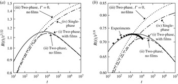
Figure 5 shows results from calculations with parameter values chosen to fit an experiment from Part 1 in the tension-dominated case. We note that, to begin with, the experimental results agree with the lubrication results for the tension-dominated system with the improved meniscus model (curve i), as expected. As the bubble grows, the difference between the boundary conditions (2.10) for an infinite cell and (2.11) for a finite cell becomes significant. Specifically, the tension in a finite cell is smaller, and hence the experimental system spreads more slowly.
On comparing the improved meniscus model (curve i) with the simple meniscus model (curve ii) in the bending- and tension-dominated cases (figure 5
a,b), we find that they initially disagree in the prediction for
 $R(t)$
, as was seen in § 3.1. However, as time passes and the peeling slows down (
 $\mathit{Ca}\rightarrow 0$
), the difference between the two interfacial models becomes negligible and the two results for
 $R$
agree. We thus expect to be able to obtain a good physical understanding of the late-time behaviour using only the simpler model (2.6).
Curve (iv) in figure 5 shows results for a single-phase system where viscous liquid is injected instead of gas. In this case, the lubrication equation (2.3) holds throughout the domain, there is no interface and the volume conservation condition (2.13) is replaced with the injection condition
 $2{\rm\pi}rq\rightarrow \dot{V}$
as
 $r\rightarrow 0$
. In order to explain the difference in behaviour between the single- and two-phase cases, we also show the two-phase case with zero surface tension (curve iii).
The two cases (iii) and (iv) with no surface tension have the same qualitative behaviour, indicating that the spreading is viscously controlled in both cases, as was argued by Lister et al. (Reference Lister, Peng and Neufeld2013). Case (ii) with non-zero surface tension is similar for
 $t\lesssim 10^{3}$
, but then undergoes a transition to a different regime. This transition must be due to the capillary pressure drop at the meniscus, as this is the only difference between models (ii) and (iii). Results (not shown) for other values of the surface tension
 ${\it\Gamma}$
indicate that the transition occurs later for smaller
 ${\it\Gamma}$
. We deduce that there should be a transition time
 $t_{1}$
(possibly of the form
 $t_{1}\propto {\it\Gamma}^{-k}t_{0}$
for some
 $k>0$
) such that surface-tension effects can be ignored for ‘moderate’ times
 $t_{0}\ll t\ll t_{1}$
, but become important for
 $t\gg t_{1}$
.
Height profiles at various times for the simple meniscus model with
 ${\it\Gamma}=0.00223$
. All quantities are non-dimensionalized by (3.1). The dotted lines indicate the position of the interface. (a) Bending,
 $t=10^{5}$
; (b) tension,
 $t=10^{5}$
; (c) bending,
 $t=10^{9}$
; (d) tension,
 $t=10^{12}$
.

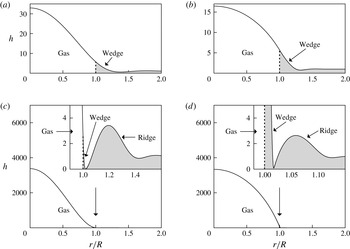
Some example profiles from the simple meniscus model are shown in figure 6. Figure 6(a,b) shows how the liquid that originally filled the cell is displaced by the bubble and accumulates in a wedge ahead of the bubble. Figure 6(c,d) reveals that, at very late times, a bottleneck forms at the tip of the liquid wedge and pushes a large ridge of liquid ahead of it. Thus, there is a second transition time
 $t_{2}$
, which divides the regime
 $t\gg t_{1}$
when surface-tension effects are important into ‘late’ times
 $t_{1}\ll t\ll t_{2}$
at which no bottleneck has formed and ‘very late’ times
 $t\gg t_{2}$
at which a bottleneck is present. We investigate the moderate- and late-time regimes together in § 4 and the very-late-time regime separately in § 5.
4. Asymptotic analysis of the wedge at moderate to late times
In this section, we present our main asymptotic analysis of the two-phase system, investigating how the capillary pressure drop across the meniscus lowers the pressure in the liquid wedge and hence affects the peeling process. The analysis applies at times
 $t_{0}\ll t\ll t_{2}$
, when the height profile is similar to those in figure 6(a,b). After some preliminary set-up in § 4.1, we solve the bending-dominated case (§ 4.2) and then the tension-dominated case (§ 4.3). We confirm the existence of a moderate-time regime (
 $t_{0}\ll t\ll t_{1}$
, when surface-tension effects are negligible) and a late-time regime (
 $t_{1}\ll t\ll t_{2}$
, when surface-tension effects are dominant), and find the time
 $t_{1}$
for transition between them. The resulting predictions for the evolution of
 $R(t)$
are validated against numerical results. Finally, the applicability of these asymptotic results to experiments is discussed in § 4.4.
Definition of variables for the asymptotic calculation.

4.1. Preliminaries for two-phase peeling
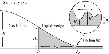
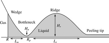
We decompose the system into three regions, as shown in figure 7: a gas bubble with radius
 $R$
and height
 $H_{b}$
, a liquid wedge (which is not necessarily triangular) with length
 $L_{w}$
and height
 $H_{w}$
, and a peeling region with length scale
 $L_{p}$
and height scale
 $H_{p}=h_{0}$
. We assume that
 $$\begin{eqnarray}R\gg L_{w}\gg L_{p},\quad H_{b}\gg H_{w}\gg h_{0}.\end{eqnarray}$$
From
 $H_{w}\gg H_{p}$
, we conclude that, like in the single-phase case, the spreading of the fluid is resisted by viscous forces near the peeling tip, while the viscous pressure drop in the wedge is negligible to leading order.
We define the position
 $R_{p}=R+L_{w}$
of the peeling tip to be where
 $h$
first attains a minimum, indicating the presence of a peeling wave. We use the heights
 $H_{n}$
at this minimum (‘the neck’) and
 $H_{r}$
at the following maximum (‘the ridge’) to identify the wave. As
 $L_{w}\ll R$
, we find that
 $R$
and
 $R_{p}$
are equal to leading order. At the interface, the height, slope and curvature are
 $$\begin{eqnarray}H_{w}(t)=h(R(t),t),\quad {\it\alpha}_{i}(t)=-h^{\prime }(R(t),t),\quad {\it\kappa}_{i}(t)=h^{\prime \prime }(R(t),t).\end{eqnarray}$$
As the lengths
 $L_{w}$
and
 $L_{p}$
are small compared with the radius
 $R$
, the effects of the radial geometry on the wedge and peeling regions are negligible at leading order, and we treat these as two-dimensional instead. We can then equate the volume
 $V_{w}$
of liquid in the wedge to the amount of liquid displaced by the gas bubble, and find the cross-sectional area
 $A_{w}$
of liquid in the wedge:
 $$\begin{eqnarray}V_{w}(t)={\rm\pi}R^{2}h_{0},\quad A_{w}(t)=\frac{V_{w}}{2{\rm\pi}R}=\frac{h_{0}R}{2}.\end{eqnarray}$$
(This expression could be used to derive the conditions (4.1) from the single assumption
 $H_{b}\gg h_{0}$
.)
4.2. Bending-dominated peeling at moderate to late times
4.2.1. Main calculation
We start by considering the case in which the elastic response of the sheet is dominated by bending forces. We seek leading-order solutions
 $h=h_{b}$
and
 $h=h_{w}$
for the gas-bubble and liquid-wedge regions respectively. We define a local position variable
 $x_{w}=R_{p}-r$
for the wedge, which ranges (backwards) between
 $L_{w}$
at the interface and
 $0$
at the peeling tip. We then write
 $h_{b}=h_{b}(r)$
and
 $h_{w}=h_{w}(x_{w})$
(with the dependence on
 $t$
being understood).
First, we investigate the interfacial conditions (2.5) and (2.6b
). We assume that the curvatures
 $h^{\prime \prime }$
in the bubble and wedge are of the same order, so that the scaling estimate
 $H_{b}/R^{2}\sim H_{w}/L_{w}^{2}\sim {\it\kappa}_{i}$
holds. The lower derivatives of the wedge solution,
 $h_{w}\sim {\it\kappa}_{i}L_{w}^{2}$
and
 $h_{w}^{\prime }\sim {\it\kappa}_{i}L_{w}$
, are then negligible compared with the corresponding scales for the bubble solution,
 $h_{b}\sim {\it\kappa}_{i}R^{2}$
and
 $h_{b}^{\prime }\sim {\it\kappa}_{i}R$
. Similarly, higher derivatives of the bubble solution are negligible compared with the corresponding scales for the wedge solution. Hence, the conditions (2.5) and (2.6b
) simplify to
 $$\begin{eqnarray}h_{b}(R)=0,\quad h_{b}^{\prime }(R)=0,\quad h_{b}^{\prime \prime }(R)={\it\kappa}_{i},\end{eqnarray}$$
 $$\begin{eqnarray}h_{w}^{\prime \prime }(L_{w})={\it\kappa}_{i},\quad h_{w}^{\prime \prime \prime }(L_{w})=0,\quad h_{w}^{\prime \prime \prime \prime }(L_{w})=-\frac{2{\it\gamma}}{Bh_{w}(L_{w})}.\end{eqnarray}$$
The fact that matching to a smaller region yields ‘clamped’ conditions
 $h=h^{\prime }=0$
on the solution for the larger region will be used again later.
The bubble region thus satisfies (4.4) together with simplified versions of the constant-pressure condition (2.4), symmetry condition (2.9) and volume constraint (2.13):
 $$\begin{eqnarray}B{\rm\nabla}^{4}h_{b}=p_{b}\quad \text{in }0<r<R,\quad h_{b}^{\prime }(0)=h_{b}^{\prime \prime \prime }(0)=0,\quad \int _{0}^{R}h_{b}(r)\,2{\rm\pi}r\,\,\text{d}r=\dot{V}t.\end{eqnarray}$$
The solution is given by
 $$\begin{eqnarray}h_{b}=\frac{3}{{\rm\pi}}\frac{\dot{V}t}{R^{2}}\left(1-\frac{r^{2}}{R^{2}}\right)^{2},\quad \frac{p_{b}}{B}=\frac{192}{{\rm\pi}}\frac{\dot{V}t}{R^{6}},\quad {\it\kappa}_{i}=h^{\prime \prime }(R)=\frac{24}{{\rm\pi}}\frac{\dot{V}t}{R^{4}}.\end{eqnarray}$$
For the liquid wedge, we argued in § 4.1 that the geometry is quasi-two-dimensional and the pressure
 $p_{w}$
is approximately constant. The matching to the small peeling region yields clamped conditions (analogous to (4.4)), and the wedge area
 $A_{w}$
is given by (4.3b
). Thus, we have the approximate equations
 $$\begin{eqnarray}Bh_{w}^{\prime \prime \prime \prime }=p_{w}(t),\quad \text{in }0<x_{w}<L_{w},\quad h_{w}(0)=h_{w}^{\prime }(0)=0,\quad \int _{0}^{L_{w}}h_{w}(x_{w})\,\,\text{d}x_{w}=A_{w}\end{eqnarray}$$
(as well as (4.5)), with
 $h_{w}(x_{w})$
,
 $p_{w}$
and
 $L_{w}$
unknown. The solution is given by
 $$\begin{eqnarray}h_{w}={\it\kappa}_{{\it\mu}}\frac{x_{w}^{2}}{2}+({\it\kappa}_{i}-{\it\kappa}_{{\it\mu}})\frac{4L_{w}x_{w}^{3}-x_{w}^{4}}{12L_{w}^{2}},\quad L_{w}=\left(\frac{30A_{w}}{2{\it\kappa}_{i}+3{\it\kappa}_{{\it\mu}}}\right)^{1/3},\quad \frac{p_{w}}{B}=-2\frac{{\it\kappa}_{i}-{\it\kappa}_{{\it\mu}}}{L_{w}^{2}},\vphantom{\mathop{\sum }_{\sum }}\end{eqnarray}$$
where
 $$\begin{eqnarray}{\it\kappa}_{{\it\mu}}^{2}={\it\kappa}_{i}^{2}-{\it\kappa}_{{\it\gamma}}^{2},\quad {\it\kappa}_{{\it\gamma}}^{2}=\frac{4{\it\gamma}}{B}.\end{eqnarray}$$
As the curvature at the tip of the wedge is
 $h_{w}^{\prime \prime }(0)={\it\kappa}_{{\it\mu}}$
, we call
 ${\it\kappa}_{{\it\mu}}$
the ‘viscous-peeling curvature’ and the peeling-by-bending solution (1.1a
) yields the peeling speed
 $$\begin{eqnarray}{\dot{R}}=0.472\frac{Bh_{0}^{1/2}{\it\kappa}_{{\it\mu}}^{5/2}}{12{\it\mu}}.\end{eqnarray}$$
The ‘capillary curvature’
 ${\it\kappa}_{{\it\gamma}}$
will be used more later.
4.2.2. Interpretation of the main result
We combine the bubble solution (4.7) and peeling result (4.10) to find
 $$\begin{eqnarray}{\dot{R}}=0.472\frac{Bh_{0}^{1/2}}{12{\it\mu}}({\it\kappa}_{i}^{2}-{\it\kappa}_{{\it\gamma}}^{2})^{5/4}=0.472\frac{Bh_{0}^{1/2}}{12{\it\mu}}\left[\left(\frac{24}{{\rm\pi}}\frac{\dot{V}t}{R^{4}}\right)^{2}-\frac{4{\it\gamma}}{B}\right]^{5/4}.\end{eqnarray}$$
Thus, the effect of surface tension is to suck the sheet down in the wedge region, so that the curvature decreases from
 ${\it\kappa}_{i}$
at the interface to the lower value
 ${\it\kappa}_{{\it\mu}}$
at the wedge tip. This slows the peeling of the sheet. Surprisingly, the result does not depend on the wedge length
 $L_{w}$
or area
 $A_{w}$
. Equation (4.11) can be integrated numerically to yield the evolution of
 $R(t)$
, but can also be solved analytically in two limits as follows.
At moderate times, our numerical results (figure 5) indicate that the effects of surface tension can be neglected. From (4.11), we see that this is appropriate if
 $$\begin{eqnarray}{\it\kappa}_{i}\gg {\it\kappa}_{{\it\gamma}}\text{or equivalently }\frac{{\it\mu}{\dot{R}}}{{\it\gamma}}\gg \left(\frac{{\it\gamma}h_{0}^{2}}{B}\right)^{1/4}.\end{eqnarray}$$
Integration of (4.11) without the surface-tension term yields the spreading law
 $$\begin{eqnarray}R(t)=1.65\left(\frac{B^{2}h_{0}\dot{V}^{5}t^{7}}{(12{\it\mu})^{2}}\right)^{1/22}\left[=1.65\,\left(\frac{t}{t_{0}}\right)^{7/22}L_{0}\right].\end{eqnarray}$$
(In this equation, and in similar equations below, we present our results both in terms of the original physical parameters and in terms of the scales
 $t_{0}$
and
 $L_{0}$
and the non-dimensional parameter
 ${\it\Gamma}$
given in (3.1) and (3.2a
).)
In this moderate-time regime, the liquid wedge is parabolic with constant curvature
 ${\it\kappa}_{i}={\it\kappa}_{{\it\mu}}$
. The capillary pressure jump across the meniscus is negligible, so the gas bubble and liquid wedge can be considered together as a constant-pressure blister, and the meniscus is simply trailing passively behind the peeling region at the velocity of the surrounding fluid. The system then behaves like a single-phase system, as was claimed by Lister et al. (Reference Lister, Peng and Neufeld2013). Indeed, the result (4.13) is identical to the single-phase result (equation (6) in Lister et al.
Reference Lister, Peng and Neufeld2013).
The interfacial curvature and spreading velocity decrease with time, and so we see from (4.12) that the moderate-time behaviour (4.11) only holds for a range of time
 $t_{0}\ll t\ll t_{1}$
(where
 $t_{1}$
is yet to be found), after which there is a transition to a different regime. Since
 ${\it\kappa}_{i}$
is prevented from falling below
 ${\it\kappa}_{{\it\gamma}}$
due to the surface-tension term in (4.11), we deduce that, at late times
 $t\gg t_{1}$
, there is a quasi-static balance
 $$\begin{eqnarray}{\it\kappa}_{i}={\it\kappa}_{{\it\gamma}}.\end{eqnarray}$$
(This condition is also found in dry adhesion problems where no fluid is present, and can be derived from a balance of elastic and surface energies, see Landau & Lifshitz (Reference Landau and Lifshitz1986, p. 45).) Solving for
 $R(t)$
using (4.7) yields
 $$\begin{eqnarray}R(t)=1.40\left(\frac{B\dot{V}^{2}t^{2}}{{\it\gamma}}\right)^{1/8}\left[=1.40\,{\it\Gamma}^{-1/8}\left(\frac{t}{t_{0}}\right)^{1/4}L_{0}\right].\end{eqnarray}$$
We observe that, although viscous forces are still important at the peeling tip, the radius of the bubble is determined by the surface-tension balance (4.14), which is independent of the viscosity. In this late-time limit, the wedge solution (4.9) reduces to the simpler form
 $$\begin{eqnarray}h_{w}={\it\kappa}_{i}\frac{4L_{w}x_{w}^{3}-x_{w}^{4}}{12L_{w}^{2}},\quad L_{w}=\left(\frac{15A_{w}}{{\it\kappa}_{i}}\right)^{1/3},\quad \frac{p_{w}}{B}=-\frac{2{\it\kappa}_{i}}{L_{w}^{2}}.\end{eqnarray}$$
To find the time
 $t_{1}$
at which the transition occurs between the moderate-time regime (4.13) and the late-time regime (4.15), we equate
 $R(t)$
between the two and find
 $$\begin{eqnarray}t_{1}=0.092\,\left(\frac{B^{3}\dot{V}^{2}(12{\it\mu})^{8}}{h_{0}^{4}{\it\gamma}^{11}}\right)^{1/6}[=0.092\,{\it\Gamma}^{-11/6}t_{0}].\end{eqnarray}$$
4.2.3. Comparison with numerical results
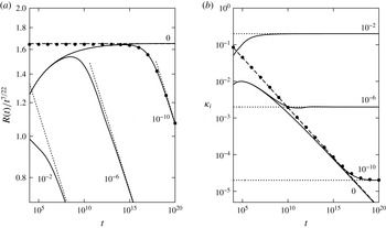
Figure 8 shows numerical and asymptotic results for various values of the surface-tension parameter
 ${\it\Gamma}$
defined in (3.2). With no surface tension (
 ${\it\Gamma}=0$
), the numerical solutions are seen to agree with the dynamic viscous-peeling prediction (4.13) at late times. When surface tension is present (
 ${\it\Gamma}\neq 0$
), the solutions initially agree with the case
 ${\it\Gamma}=0$
, but then start to transition one by one (in order of decreasing
 ${\it\Gamma}$
) towards the quasi-static surface-tension-controlled solution (4.15). To verify the results (4.10) describing the transition between the two limiting cases, we integrated (4.11) numerically, and again obtained excellent agreement with the full numerical results (see figure 8, points).
Evolution of (a) the radius
 $R(t)$
and (b) the interfacial curvature
 ${\it\kappa}_{i}$
, for bending-dominated peeling, using non-dimensional variables (3.1a
). Numerical results (solid lines) for four values of the surface tension
 ${\it\Gamma}$
as shown. Asymptotic results: moderate times ((4.13), dashed line), late times ((4.15), dotted line) and transition (numerical solution of (4.11), points,
 ${\it\Gamma}=10^{-10}$
).

Given the results for the radius
 $R(t)$
, asymptotic predictions for other key quantities, such as the central cell height
 $h_{b}(r=0)$
or the pressure
 $p_{b}$
in the bubble, can be obtained by substitution into the bubble solution (4.7). These predictions also show excellent agreement with the numerical results (not shown).
We conclude that our asymptotic method can predict the time evolution of the bubble radius across two different regimes: the bubble spreads at moderate times according to the viscous-peeling law (1.1a ), with surface-tension effects being negligible, and at late times according to the quasi-static surface-tension balance (4.14). The transition between the two is described by the modified peeling law (4.10c ).
4.3. Tension-dominated peeling at moderate to late times
We now turn to the case when the tension term
 $p_{T}=-\boldsymbol{{\rm\nabla}}\boldsymbol{\cdot }(T\boldsymbol{{\rm\nabla}}h)$
dominates over the bending term
 $p_{B}=B{\rm\nabla}^{4}h$
in (2.2). This occurs when the horizontal length scales of the bubble, wedge and peeling regions are much larger than the bending–tension length scale
 $L_{BT}=\sqrt{B/T}$
. Although there is a boundary layer of length
 $O(L_{BT})$
near the interface where the bending is important, its effect on the larger bubble and wedge regions is negligible (see figure 4
b). Thus, the appropriate dynamic interfacial conditions are a capillary pressure jump in
 $p_{T}$
and continuity of the lower-order derivatives
 $h$
and
 $h^{\prime }$
.
The dependence of the peeling speed (1.1b
) on the length-scale ratio
 ${\it\Delta}=L_{o}/L_{pT}$
, where
 $L_{o}$
is the length scale of the relevant outer region (the wedge in this case) and
 $L_{pT}$
is the peeling length scale, raises two technical issues. First, the outer length scale
 $L_{o}$
can be defined with any
 $O(1)$
multiplicative constant without affecting the leading-order analysis. Second, the peeling length scale
 $L_{pT}=(T/12{\it\mu}{\dot{R}})^{1/3}h_{0}$
depends on the peeling speed, so that (1.1b
) is an implicit equation for
 ${\dot{R}}$
. These issues are addressed by rewriting (1.1b
) as
 $$\begin{eqnarray}{\dot{R}}=\frac{T{\it\alpha}_{b}^{3}}{12{\it\mu}\ln _{\ast }[(cL_{o}{\it\alpha}_{b}/h_{0})^{3}]},\end{eqnarray}$$
where
 $c$
represents a choice of
 $O(1)$
constant and we use
 $\ln _{\ast }(x)$
to denote the Lambert
 $W$
-function, defined by
 $\ln _{\ast }(x)\exp [\ln _{\ast }(x)]=x$
, which has the asymptotic behaviour
 $$\begin{eqnarray}\ln _{\ast }(x)\sim \ln x-\ln \ln x+\frac{\ln \ln x}{\ln x}+O\left(\frac{(\ln \ln x)^{2}}{(\ln x)^{2}}\right)\quad \text{as }x\rightarrow \infty .\end{eqnarray}$$
Previous publications (e.g. Lister et al.
Reference Lister, Peng and Neufeld2013; Hewitt et al.
Reference Hewitt, Balmforth and De Bruyn2014) have used estimates for
 ${\it\Delta}$
that are equivalent to the approximation
 $\ln _{\ast }(x)\approx \ln x$
, which leaves a rather large relative error of size
 $O(\ln \ln {\it\Delta}/\ln {\it\Delta})$
. Using (4.18) with an arbitrary choice of
 $c$
(such as
 $c=1$
) reduces the error to
 $O(1/\ln {\it\Delta})$
. As this error is still only logarithmically small, it is useful (and sometimes necessary) to calculate the first correction, from which we can determine a unique value of
 $c$
that reduces the error to
 $O(1/(\ln {\it\Delta})^{2})$
. For clarity, we simply state the value of
 $c$
in the main text, and leave the detailed calculations of the various instances of
 $c$
to appendix A.
As most of the reasoning is similar to the bending-dominated case § 4.2, we will be brief and only go into detail where the analysis is different.
4.3.1. Main calculation
We again make use of the asymptotic regions shown in figure 7. Using the same bubble and wedge variables
 $h_{b}(r)$
and
 $h_{w}(x_{w})$
as in § 4.2.1, the appropriate interfacial conditions analogous to (4.4) and (4.5), based on matching slopes
 $h^{\prime }$
, are
 $$\begin{eqnarray}h_{b}(R)=0,\quad -h_{b}^{\prime }(R)=h_{w}^{\prime }(L_{w})={\it\alpha}_{i},\quad h_{w}^{\prime \prime }(L_{w})=\frac{2{\it\gamma}}{Th_{w}(L_{w})}.\end{eqnarray}$$
The bubble satisfies the further equations
 $$\begin{eqnarray}-\boldsymbol{{\rm\nabla}}\boldsymbol{\cdot }(T\boldsymbol{{\rm\nabla}}h_{b})=p_{b}\quad \text{in }0<r<R,\quad h_{b}^{\prime }(0)=0,\quad \int _{0}^{R}h_{b}(r)\,2{\rm\pi}r\,\,\text{d}r=\dot{V}t.\end{eqnarray}$$
Unlike in the bending-dominated case where
 $B$
is a constant, the tension
 $T(r,t)$
is variable and is coupled to the height profile by (2.2). We solve the coupled system following the method of Lister et al. (Reference Lister, Peng and Neufeld2013). Far ahead of the bubble, the sheet is undisturbed and the solution to (2.2) satisfying the far-field condition (2.11d
) is
 $T\propto r^{-2}$
. As the wedge and peeling regions are short compared with the bubble, a scaling analysis reveals that the variations in
 $T$
and
 $T^{\prime }$
across those regions are negligible to leading order. The leading-order solution
 $T=T_{b}(r)$
in the bubble region should thus match directly onto the far-field solution at the bubble edge. The appropriate equations are
 $$\begin{eqnarray}\frac{1}{r}(r^{3}T_{b}^{\prime })^{\prime }=-\frac{Ed}{2}h_{b}^{\prime 2}\quad \text{in }0<r<R,\quad T_{b}^{\prime }(0)=0,\quad T_{b}^{\prime }(R)=-2\frac{T_{b}(R)}{R}.\end{eqnarray}$$
Equations (4.21) and (4.22) are solved numerically to yield
 $$\begin{eqnarray}h_{b}=\frac{\dot{V}t}{R^{2}}{\hat{h}}_{b}\left(\frac{r}{R}\right),\quad T_{b}=\frac{Ed\dot{V}^{2}t^{2}}{R^{6}}\hat{T}_{b}\left(\frac{r}{R}\right),\quad p_{b}=0.328\frac{Ed\dot{V}^{3}t^{3}}{R^{10}},\end{eqnarray}$$
 $$\begin{eqnarray}{\it\alpha}_{i}=-h_{b}^{\prime }(R)=1.59\frac{\dot{V}t}{R^{3}},\quad T_{i}=T_{b}(R)=0.103\frac{Ed\dot{V}^{2}t^{2}}{R^{6}},\end{eqnarray}$$
where
 ${\hat{h}}_{b}$
and
 $\hat{T}_{b}$
are unique non-dimensional solution profiles. These results differ from those of Lister et al. (Reference Lister, Peng and Neufeld2013) by a few per cent.
As the variation in tension across the wedge region is negligible, the tension takes the interfacial value
 $T_{i}$
there. The wedge thus satisfies the equations
 $$\begin{eqnarray}-T_{i}h_{w}^{\prime \prime }=p_{w}(t)\text{ in }0<x_{w}<L_{w},\quad h_{w}(0)=0,\quad \int _{0}^{L_{w}}h_{w}(x_{w})\,\text{d}x_{w}=A_{w},\end{eqnarray}$$
and matching conditions (4.20), with solution
 $$\begin{eqnarray}h_{w}={\it\alpha}_{{\it\mu}}x_{w}+({\it\alpha}_{i}-{\it\alpha}_{{\it\mu}})\frac{x_{w}^{2}}{2L_{w}},\quad L_{w}=\left(\frac{6A_{w}}{{\it\alpha}_{i}+2{\it\alpha}_{{\it\mu}}}\right)^{1/2},\quad \frac{p_{w}}{T_{i}}=-\frac{{\it\alpha}_{i}-{\it\alpha}_{{\it\mu}}}{L_{w}},\end{eqnarray}$$
again expressed in terms of auxiliary variables
 $$\begin{eqnarray}{\it\alpha}_{{\it\mu}}^{2}={\it\alpha}_{i}^{2}-{\it\alpha}_{{\it\gamma}}^{2},\quad {\it\alpha}_{{\it\gamma}}^{2}=\frac{4{\it\gamma}}{T_{i}}.\end{eqnarray}$$
This yields, from (4.18), the peeling speed (with
 $c$
derived in § A.2)
 $$\begin{eqnarray}{\dot{R}}=\frac{T_{i}{\it\alpha}_{{\it\mu}}^{3}}{12{\it\mu}\ln _{\ast }[(cL_{w}{\it\alpha}_{{\it\mu}}/h_{0})^{3}]},\quad c=0.281\frac{2{\it\alpha}_{{\it\mu}}}{{\it\alpha}_{i}+{\it\alpha}_{{\it\mu}}}.\end{eqnarray}$$
4.3.2. Interpretation of the main result
As in the bending-dominated case (§ 4.2.2), we find that the capillary forces produce a negative pressure in the wedge which sucks down the sheet and reduces the slope
 ${\it\alpha}_{{\it\mu}}$
seen by the peeling solution at the tip, thus reducing the peeling speed. Again, the reduction from the interfacial slope
 ${\it\alpha}_{i}$
to the viscous-peeling slope
 ${\it\alpha}_{{\it\mu}}$
does not depend on
 $L_{w}$
or
 $A_{w}$
. However, the peeling speed does depend on
 $L_{w}$
(and hence
 $A_{w}$
), albeit only logarithmically.
At moderate times
 $t_{0}\ll t\ll t_{1}$
(with
 $t_{1}$
to be found), we again expect surface tension to be negligible. Due to the dependence of
 ${\it\alpha}_{{\it\gamma}}$
on
 $T_{i}\sim Ed{\it\alpha}_{i}^{2}$
, the appropriate condition
 ${\it\alpha}_{i}\gg {\it\alpha}_{{\it\gamma}}$
can instead be written as
 $$\begin{eqnarray}{\it\alpha}_{i}\gg \left(\frac{{\it\gamma}}{Ed}\right)^{1/4}\quad \text{or equivalently}\quad \frac{{\it\mu}{\dot{R}}}{{\it\gamma}}\gg \left(\frac{{\it\gamma}}{Ed}\right)^{1/4}\end{eqnarray}$$
(after neglecting a logarithmic factor in the second expression). To find the moderate-time spreading rate, we integrate (4.26c ) using (4.23d,e ) and (4.26a,b ) without the surface-tension term, and obtain
 $$\begin{eqnarray}\displaystyle & \displaystyle R(t)=1.02\left(\frac{Ed\dot{V}^{5}}{12{\it\mu}}\frac{t^{6}}{\ln _{\ast }[c(12{\it\mu}\dot{V}^{3}t^{2}/Edh_{0}^{8})^{3/13}]}\right)^{1/16},\quad c=0.0242, & \displaystyle\end{eqnarray}$$
 $$\begin{eqnarray}\displaystyle & \displaystyle \left[R(t)=1.02\,\frac{(t/t_{0})^{3/8}}{\ln _{\ast }[c(t/t_{0})^{6/13}]^{1/16}}L_{0}\right]. & \displaystyle\end{eqnarray}$$
In this moderate-time limit, the wedge is triangular with constant slope
 ${\it\alpha}_{i}={\it\alpha}_{{\it\mu}}$
. Again, this case allows the gas bubble and liquid wedge to be viewed together as a constant-pressure blister and analogies to be drawn to the single-phase result. However, the peeling speed now depends on the outer length scale, which is
 $R$
for single-phase spreading but
 $L_{w}$
for two-phase spreading. Hence, it can be shown that the leading-order numerical coefficient in (4.28) is different (as was argued by Lister et al.
Reference Lister, Peng and Neufeld2013). The main exponent,
 $R(t)\propto t^{3/8}$
, remains the same (cf. equation (18) in Lister et al.
Reference Lister, Peng and Neufeld2013). This behaviour is also observed in figure 14 of Part 1.
Again, the late-time behaviour of the system is given by a quasi-static surface-tension balance
 $$\begin{eqnarray}{\it\alpha}_{i}={\it\alpha}_{{\it\gamma}}\quad \Rightarrow \quad {\it\alpha}_{i}=3.15\,\left(\frac{{\it\gamma}}{Ed}\right)^{1/4},\end{eqnarray}$$
which yields
 $$\begin{eqnarray}R(t)=0.797\,\left(\frac{Ed\dot{V}^{4}t^{4}}{{\it\gamma}}\right)^{1/12}\left[=0.797{\it\Gamma}^{-1/12}\left(\frac{t}{t_{0}}\right)^{1/3}L_{0}\right].\end{eqnarray}$$
In this late-time limit, the wedge solution (4.25) reduces to the parabolic solution
 $$\begin{eqnarray}h_{w}(x_{w})={\it\alpha}_{i}\frac{x_{w}^{2}}{2L_{w}},\quad L_{w}=\left(\frac{6A_{w}}{{\it\alpha}_{i}}\right)^{1/2},\quad \frac{p_{w}}{T}=-\frac{{\it\alpha}_{i}}{L_{w}}.\end{eqnarray}$$
The transition time between the moderate- and late-time behaviours is
 $$\begin{eqnarray}\displaystyle & \displaystyle \hspace{-18.0pt}t_{1}=4.57\times 10^{-4}\left(\frac{(12{\it\mu})^{3}Ed\dot{V}}{{\it\gamma}^{4}}\ln _{\ast }\left[c\left(\frac{12{\it\mu}\dot{V}}{{\it\gamma}h_{0}^{2}}\right)^{3}\right]\right)^{1/2}\!,\quad c=2.52\times 10^{-9}, & \displaystyle\end{eqnarray}$$
 $$\begin{eqnarray}\displaystyle & \displaystyle [t_{1}=4.57\times 10^{-4}~{\it\Gamma}^{-2}\ln _{\ast }(c{\it\Gamma}^{-3})^{1/2}t_{0}].\qquad & \displaystyle\end{eqnarray}$$
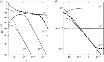
4.3.3. Comparison with numerical results
Figure 9 (analogous to figure 8) shows numerical and asymptotic results for various values of the surface-tension parameter
 ${\it\Gamma}$
(defined in (3.2)). The observations and conclusions for the bending-dominated case in § 4.2.3 carry over to the tension-dominated case here.
Evolution of (a) the radius
 $R(t)$
and (b) the interfacial slope
 ${\it\alpha}_{i}$
, for tension-dominated peeling, using non-dimensional variables (3.1b
). Numerical results (solid lines) for four values of the surface tension
 ${\it\Gamma}$
as shown. Asymptotic results: moderate times ((4.28) with
 $c$
as given, dashed line, or arbitrary
 $c=1$
, dash-dotted line), late times ((4.30), dotted lines) and transition (numerical solution of (4.23), (4.26), points,
 ${\it\Gamma}=10^{-10}$
).

We show two asymptotic results for the case
 ${\it\Gamma}=0$
in figure 9. As expected, inclusion of the first-order correction with
 $c$
as given in (4.28) yields a noticeably more accurate solution than the leading-order result with
 $c=1$
.
4.4. Application of moderate-to-late-time results to experiments
To aid understanding, the asymptotic analyses in §§ 4.2 and 4.3 were presented for some simple physical conditions. Before applying our understanding to the results from Part 1 in § 4.4.3, we first discuss how to generalize the analyses to allow films of liquid being deposited on the cell walls using the improved meniscus condition (§ 4.4.1) and how to deal with both bending and tension forces being important (§ 4.4.2).
4.4.1. The improved meniscus condition
Our main results (4.10), (4.26) depend on the dynamic interfacial condition (2.6b
) which describes the pressure drop across the meniscus, but not on the kinematic condition (2.6a
) which describes the amount of fluid left behind the advancing meniscus (apart from the weak logarithmic dependence on the wedge length
 $L_{w}$
in the tension-dominated case). Since the dynamic condition for the improved meniscus model (2.8) can be obtained from that of the simple model (2.6) by the substitution
 ${\it\gamma}\rightarrow {\it\gamma}f_{2}(\mathit{Ca})$
, the peeling laws for the improved model are again (4.10), (4.26) but with different capillary curvature or slope given by
 $$\begin{eqnarray}{\it\kappa}_{{\it\gamma}}^{2}=\frac{4{\it\gamma}f_{2}(\mathit{Ca})}{B},\quad {\it\alpha}_{{\it\gamma}}^{2}=\frac{4{\it\gamma}f_{2}(\mathit{Ca})}{T_{i}},\quad \mathit{Ca}={\it\mu}{\dot{R}}/{\it\gamma}.\end{eqnarray}$$
The peeling laws then become implicit equations for the peeling speed
 ${\dot{R}}$
which must be solved numerically. However, all of the physical effects discussed throughout §§ 4.2 and 4.3 still hold.
4.4.2. Both bending and tension
Our analysis is also easily extended to the case when the bubble is tension-dominated (i.e.
 $R\gg L_{BT}$
) while the peeling region is bending-dominated (i.e.
 $L_{pB}\ll L_{BT}$
). The sheet deflection in the wedge region is then governed by
 $$\begin{eqnarray}-T_{i}h_{w}^{\prime \prime }+Bh_{w}^{\prime \prime \prime \prime }=p_{w},\quad h_{w}(0)=h_{w}^{\prime }(0)=0.\end{eqnarray}$$
On the bubble side of the meniscus, there is a bending–tension boundary layer in which
 $h^{\prime }\approx C\text{e}^{(r-R)/L_{BT}}+{\it\alpha}_{i}$
, where
 $C$
is a constant to be determined. Here,
 ${\it\alpha}_{i}$
is the apparent interfacial slope that the bubble solution would have in the absence of the boundary layer, and is thus again given by (4.23). Applying the interfacial conditions (2.6) between the wedge and boundary-layer solutions and solving yields
 $$\begin{eqnarray}{\it\kappa}_{{\it\mu}}^{2}=\frac{{\it\alpha}_{i}^{2}}{L_{BT}^{2}}-{\it\kappa}_{{\it\gamma}}^{2}\quad \Rightarrow \quad {\dot{R}}=0.472\frac{Bh_{0}^{1/2}}{12{\it\mu}L_{BT}^{5/2}}({\it\alpha}_{i}^{2}-{\it\alpha}_{{\it\gamma}}^{2})^{5/4}.\end{eqnarray}$$
At moderate times, when
 ${\it\alpha}_{{\it\gamma}}$
is negligible, we recover the bending–tension hybrid viscous-peeling result found by Lister et al. (Reference Lister, Peng and Neufeld2013), with
 $$\begin{eqnarray}R(t)=0.913\left(\frac{E^{5}d^{5}h_{0}^{2}\dot{V}^{20}}{(12{\it\mu})^{4}B}\right)^{1/64}t^{3/8}.\end{eqnarray}$$
At late times, we recover the quasi-static balance
 ${\it\alpha}_{i}={\it\alpha}_{{\it\gamma}}$
(4.29) and power law
 $R(t)\propto t^{1/3}$
(4.30) from the tension-dominated case.
4.4.3. Explanation of results from Part 1
Our asymptotic analyses have confirmed the claim by Lister et al. (Reference Lister, Peng and Neufeld2013) that, at early times when surface-tension effects are negligible, the spreading of the bubble is viscously controlled and very similar to the single-phase case. In particular, we recover two power laws (4.28) and (4.36) with the same main exponent,
 $R(t)\propto t^{3/8}$
, which were found by Lister et al. (Reference Lister, Peng and Neufeld2013) to apply when the central bubble (or blister) is tension-dominated (which is when
 $H_{b}\gg d$
) and the peeling region is either tension- or bending-dominated. The (two-phase) experiments in Part 1 belong to these regimes or a transition between them, and indeed were found to follow this power law approximately.
In Part 1, it was noted that, perhaps surprisingly, the simple meniscus model (2.6) is in good agreement with the Navier–Stokes results regarding the height profile (and the pressure profile in the peeling region), even when there is a noticeable difference for the bubble radius (and gas pressure). The asymptotic analysis reveals why. We see from the pressure profiles (figure 2) that the interfacial pressure jump is (somewhat) small compared with the peeling pressure scales. Hence, as argued in § 4.2.2, the spreading process is controlled by the viscous forces at the peeling tip, while the meniscus is passively advected with the mean flow behind it. Thus, the overall height profile is not expected to depend sensitively on the conditions applied at the meniscus, even though the internal distribution of the two fluids differs.
5. Asymptotic analysis of the ridge and bottleneck at very late times
At very late times, the system transitions to a bottleneck-and-ridge structure, as seen in figure 6(c,d), which is different from the structure assumed for the asymptotic analysis in § 4. However, the late-time predictions (4.15), (4.30) for
 $R(t)$
remain valid after the transition (as seen in figures 8 and 9), indicating that the wedge solutions (4.16), (4.31) also remain valid. We confirm this by performing an asymptotic analysis for the very-late-time regime based on (4.15), (4.16), (4.30) and (4.31).
In this limit, surface tension plays a dominant role and the spreading is quasi-statically controlled. The peeling speed
 ${\dot{R}}$
is thus no longer an unknown (to be determined by a viscous-peeling condition), but is instead given by differentiating (4.15) and (4.30).
We first use our asymptotic analysis to predict the time
 $t_{2}$
of transition to the bottleneck-and-ridge regime (§ 5.1), and then analyse the structure in both the bending- and tension-dominated cases (§§ 5.2 and 5.3). Finally, we discuss the application of our results to the experiments in Part 1 (§ 5.4).
5.1. Transition towards the very-late-time regime
We investigate when the analysis in §§ 4.2.1 and 4.3.1 fails, as time increases and the system approaches the surface-tension-controlled solution (4.15), (4.16), (4.30), (4.31). It is straightforward to check that the point of failure for both the bending- and the tension-dominated cases is in the matching between the peeling region and the wedge region.
5.1.1. Bending-dominated case
The peeling region has a length scale
 $L_{pB}=(Bh_{0}^{3}/12{\it\mu}{\dot{R}})^{1/5}$
, which increases as the spreading decelerates (or equivalently
 ${\it\kappa}_{{\it\mu}}\rightarrow 0$
). The peeling-by-bending solution (1.1a
) relies on matching the second derivative
 ${\it\kappa}_{{\it\mu}}=h^{\prime \prime }$
between the two regions, while the third derivative of the wedge solution
 $$\begin{eqnarray}{\it\phi}_{w}=h_{w}^{\prime \prime \prime }(0)=\frac{2{\it\kappa}_{{\it\gamma}}}{L_{w}}\end{eqnarray}$$
must be small compared with the corresponding peeling scale
 $h_{p}^{\prime \prime \prime }\sim h_{0}/L_{pB}^{3}$
. This condition eventually fails due to
 $L_{pB}^{3}$
increasing faster than
 $L_{w}$
. Equating
 ${\it\phi}_{w}$
with
 $h_{0}/L_{pB}^{3}$
yields the transition time
 $$\begin{eqnarray}t_{2}\sim 0.0184\left(\frac{(12{\it\mu})^{36}B^{11}\dot{V}^{14}}{h_{0}^{28}{\it\gamma}^{47}}\right)^{1/22}\quad [=0.0184\,{\it\Gamma}^{-47/22}t_{0}].\end{eqnarray}$$
We note that this is indeed much later than the transition time (4.17) between the ‘moderate’ and ‘late’ regimes for
 ${\it\Gamma}\ll 1$
.
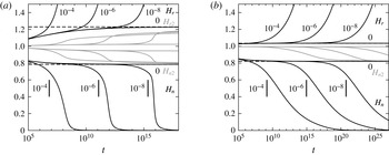
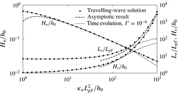
Evolution of the heights
 $H_{n}$
and
 $H_{r}$
of the first neck and ridge for (a) bending- and (b) tension-dominated peeling, using non-dimensional variables (3.1). Numerical results (solid lines) for four values of the surface tension
 ${\it\Gamma}$
as shown. Asymptotic values (dashed lines) for viscous peeling (1.1) and predictions for transition time ((5.2) and (5.4), vertical lines). Also shown are numerical results for the heights
 $H_{n2}$
and (bending only)
 $H_{r2}$
of the second neck and ridge (grey lines).

Figure 10(a) shows the time evolution of the heights
 $H_{n}$
and
 $H_{r}$
at the first neck and ridge (figure 7). The peeling-by-bending travelling-wave solution (1.1a
) has
 $H_{n}=0.785h_{0}$
and
 $H_{r}=1.230h_{0}$
, and we find (as in figure 8) that this limit is achieved by the solution with
 ${\it\Gamma}=0$
. For
 ${\it\Gamma}\neq 0$
, the solutions again follow this solution initially before they depart one by one in order of decreasing
 ${\it\Gamma}$
. For small
 ${\it\Gamma}$
, the departure is seen to be quite abrupt, indicating a fairly sudden transition to the bottleneck-and-ridge regime. The transition does indeed occur close to our predicted times (5.2).
Finally, we note that after each transition, the heights of the next neck and ridge (shown in grey in figure 10) tend towards the original (i.e. viscous peeling by bending) neck and ridge values. This suggests that after the first ridge grows large, the front of this ridge is again described by a viscous peeling-by-bending solution.
We can now explain why the numerical results for
 $R(t)$
still agree with our asymptotic late-time prediction (4.15) from § 4. First, the peeling region is replaced by a bottleneck which is also much smaller in height than the wedge region, and so the wedge equations (4.8) still hold. Second, the curvature
 ${\it\kappa}_{{\it\mu}}$
at the tip of the wedge must be effectively zero (on the scale of the wedge), or else the original analysis from § 4.2.1 holds. Hence, the wedge solution (4.16) holds, and consequently the evolution of the bubble is still given by the quasi-static condition (4.14).
5.1.2. Tension-dominated case
As in § 5.1.1, we expect the analysis in § 4.3.1 to fail as the spreading slows down and the peeling length scale
 $L_{pT}=(T_{i}/12{\it\mu}{\dot{R}})^{1/3}h_{0}$
grows. This time, the condition that fails is that the curvature
 $$\begin{eqnarray}{\it\kappa}_{w}=h_{w}^{\prime \prime }(0)=\frac{{\it\alpha}_{{\it\gamma}}}{L_{w}}\end{eqnarray}$$
of the wedge solution should be small compared with the peeling curvature scale
 $h_{p}^{\prime \prime }\sim h_{0}/L_{pT}^{2}$
. Equating the two quantities yields the prediction
 $$\begin{eqnarray}t_{2}\sim 0.00359\,\left(\frac{(12{\it\mu})^{24}E^{5}d^{5}\dot{V}^{14}}{h_{0}^{18}{\it\gamma}^{29}}\right)^{1/10}[=0.00359\,{\it\Gamma}^{-29/10}t_{0}]\end{eqnarray}$$
for the transition time.
Figure 10(b) shows the time evolution of the neck and ridge height for a range of values of the surface-tension parameter
 ${\it\Gamma}$
. The solution with
 ${\it\Gamma}=0$
follows the asymptotic predictions (
 $H_{n}=0.822\,h_{0}$
and
 $H_{r}=1.035\,h_{0}$
) for viscous peeling by pulling (1.1b
), while the solutions with
 ${\it\Gamma}\neq 0$
slowly transition away one by one close to the times predicted in (5.4).
We can make the same argument as in § 5.1.1 that the bottleneck-and-ridge structure still involves a dominant-surface-tension wedge region (4.31), which explains why the radius
 $R(t)$
is still accurately predicted by the quasi-static result (4.30).
5.2. Bending-dominated peeling at very late times
To confirm our argument in the last paragraph of § 5.1.1, we analyse the full bottleneck-and-ridge structure based on the schematic in figure 11. The wedge is assumed to be described by the strong-surface-tension solution (4.16), whose behaviour at the wedge tip (i.e. the bottleneck) is cubic with coefficient
 ${\it\phi}_{w}$
given by (5.1). As the horizontal extent of the bottleneck-and-ridge structure is small compared with the radius
 $R(t)$
, the geometry is two-dimensional and all parts are moving outward at the same speed
 ${\dot{R}}$
(to leading order).
Structure at the bubble tip at very late times.

The slow spreading speed
 ${\dot{R}}$
does not supply enough liquid to the bottleneck to keep the neck height
 $H_{n}$
at
 $O(h_{0})$
, so the capillary suction brings down the height to
 $H_{n}\ll h_{0}$
. This reduces the leftward flux
 $q_{n}$
through the neck, with the consequence that the liquid displaced by the bubble now accumulates in a large ridge ahead of the neck, rather than in the wedge behind it. Our numerical results further indicate (and we will later check) that
 $q_{n}$
decays sufficiently fast that the volume of liquid in the wedge tends to a finite value
 $V_{w}$
. Equation (4.3) is thus replaced in the very-late-time limit by
 $$\begin{eqnarray}V_{w}=\text{constant},\quad A_{w}=\frac{V_{w}}{2{\rm\pi}R},\quad V_{r}={\rm\pi}R^{2}h_{0},\quad A_{r}=\frac{V_{r}}{2{\rm\pi}R}=\frac{Rh_{0}}{2},\end{eqnarray}$$
where the value of
 $V_{w}$
depends on the initial evolution and can be crudely estimated by the amount
 ${\rm\pi}R(t_{2})^{2}h_{0}$
of displaced liquid at the time of transition (5.2) to the bottleneck-and-ridge regime.
For the ridge, we again define a local position variable and leading-order solution
 $$\begin{eqnarray}x_{r}=r-R_{p},\quad h_{r}(x_{r})\approx h(r).\end{eqnarray}$$
As the ridge is large (
 $h_{r}\gg h_{0}$
), its pressure
 $p_{r}$
is constant to leading order, and the matching to the smaller neck and peeling regions at both ends results in clamped boundary conditions. The area
 $A_{r}$
of the ridge is given by (5.5). This yields the equations
 $$\begin{eqnarray}Bh_{r}^{\prime \prime \prime \prime }=p_{r},\quad h_{r}=h_{r}^{\prime }=0\quad \text{at }x_{r}=0,~L_{r},\quad \int _{0}^{L_{r}}h_{r}(x_{r})\,\,\text{d}x_{r}=A_{r}.\end{eqnarray}$$
We solve for the profile
 $h_{r}(x_{r})$
and find the curvature
 ${\it\kappa}_{r}$
at both ends of the ridge:
 $$\begin{eqnarray}h_{r}(x_{r})=\frac{30A_{r}}{L_{r}^{5}}x_{r}^{2}(L_{r}-x_{r})^{2},\quad {\it\kappa}_{r}=h_{r}^{\prime \prime }(0)=h_{r}^{\prime \prime }(L_{r})=\frac{60A_{r}}{L_{r}^{3}}.\end{eqnarray}$$
At the front of the ridge, figure 10(a) indicates that there is a viscous peeling-by-bending solution (1.1a
). Since the speed
 ${\dot{R}}$
is given, (1.1a
) yields a condition on
 ${\it\kappa}_{r}$
, which we combine with (5.8) to find
 $$\begin{eqnarray}L_{r}=3.54\,A_{r}^{1/3}\left(\frac{Bh_{0}^{1/2}}{12{\it\mu}{\dot{R}}}\right)^{2/15}=3.62\,\left(\frac{B^{19}h_{0}^{48}\dot{V}^{6}t^{22}}{(12{\it\mu})^{16}{\it\gamma}^{3}}\right)^{1/120},\end{eqnarray}$$
where the final expression is obtained by substituting from (5.5) for
 $A_{r}$
and from the late-time result (4.15) for
 $R(t)$
.
We now seek a bottleneck solution
 $h_{n}(x_{n}=r-R_{p})=h(r)$
that joins the wedge region (with
 $h\sim -{\it\phi}_{w}x_{n}^{3}/6$
) to the ridge region (with
 $h\sim {\it\kappa}_{r}x_{n}^{2}/2$
). The detailed calculation of this solution is given in appendix B, and numerical results are shown in figure 14. Using the assumption that
 $V_{w}$
tends to a constant, we show that the quantity
 ${\hat{c}}$
defined in (B 6b
) tends to infinity, allowing us to use the asymptotic result (B 7a
). This yields the small rate of change (which was ignored earlier)
 $$\begin{eqnarray}\dot{V}_{w}=2{\rm\pi}Rq_{n}=0.568\,\left(\frac{(12{\it\mu})^{9}R^{7}{\dot{R}}^{21}V_{w}^{5}}{B^{9}{\it\kappa}_{{\it\gamma}}^{20}}\right)^{1/12}=0.0345\,\left(\frac{B^{9}(12{\it\mu})^{18}V_{w}^{10}\dot{V}^{14}}{{\it\gamma}^{27}t^{28}}\right)^{1/24},\end{eqnarray}$$
where we have used
 ${\it\kappa}_{{\it\gamma}}=\sqrt{4{\it\gamma}/B}$
and the late-time result (4.15) for
 $R(t)$
. Integrating this differential equation confirms that
 $V_{w}$
does tend to a constant.
Comparison between numerical and asymptotic results for bending-dominated peeling at very late times, using non-dimensional variables (3.1a
) (
 ${\it\Gamma}=10^{-6}$
), showing the bubble radius
 $R$
(4.15), the expression
 $(V_{r}/{\rm\pi})^{1/2}$
depending on the ridge volume (5.5c
), the ridge length
 $L_{r}$
(5.9) and the combination
 $V_{w}^{1/12}/\dot{V}_{w}^{1/5}$
of the wedge volume and its rate of change (5.10).

We compare numerical results with some asymptotic predictions in figure 12. The excellent agreement after the transition near
 $t\sim 10^{12}t_{0}$
confirms the validity of our asymptotic calculations.
5.3. Tension-dominated peeling at very late times
Based on figure 6(d), we repeat the calculation in § 5.2, again using the schematic shown in figure 11, with the whole structure moving at the same prescribed speed
 ${\dot{R}}$
, given by (4.30), at leading order. The wedge is described by the strong-surface-tension solution (4.31) with curvature
 ${\it\kappa}_{w}$
given by (5.3) at the tip.
Unlike in § 5.2, we find that the narrow bottleneck can let through the large flux
 $q_{n}={\dot{R}}h_{0}$
, so that the displaced liquid may keep accumulating in the wedge, instead of transitioning to accumulating in the ridge. The whole bottleneck-and-ridge structure then forms a travelling-wave solution (which is different from the original (1.1b
)), which is part of a family of solutions calculated numerically by McEwan & Taylor (Reference McEwan and Taylor1966).
Analogously to § 5.2, the local variables (5.6) for the ridge satisfy
 $$\begin{eqnarray}-T_{i}h_{r}^{\prime \prime }=p_{r},\quad h_{r}=0\quad \text{at }x_{r}=0,~L_{r},\quad \int _{0}^{L_{r}}h_{r}(x_{r})\,\,\text{d}x_{r}=A_{r},\end{eqnarray}$$
with solution profile and tip slope
 $$\begin{eqnarray}h_{r}(x_{r})=\frac{6A_{r}}{L_{r}^{3}}x_{r}(L_{r}-x_{r}),\quad {\it\alpha}_{r}=h_{r}^{\prime }(0)=-h_{r}^{\prime }(L_{r})=\frac{6A_{r}}{L_{r}^{2}}.\end{eqnarray}$$
Matching to a peeling-by-pulling tip yields (see § A.3)
 $$\begin{eqnarray}{\dot{R}}=\frac{T_{i}{\it\alpha}_{r}^{3}}{12{\it\mu}\ln _{\ast }[(c{\it\alpha}_{r}L_{r}/h_{0})^{3}]},\quad c=0.281,\end{eqnarray}$$
which can be solved for
 $L_{r}$
given
 $A_{r}$
:
 $$\begin{eqnarray}L_{r}=2.75\left\{\frac{T_{i}A_{r}^{3}}{12{\it\mu}{\dot{R}}\ln _{\ast }[c(12{\it\mu}{\dot{R}}/T_{i})(A_{r}/h_{0}^{2})^{3}]}\right\}^{1/6},\quad c=0.213.\end{eqnarray}$$
The bottleneck solution
 $h_{n}(x_{n}=r-R_{p})=h(r)$
joins the wedge, which approaches quadratically with
 $h_{n}\sim {\it\kappa}_{w}x_{n}^{2}/2$
, to the ridge, which approaches linearly with
 $h\sim {\it\alpha}_{r}x_{n}$
. Unlike in the bending-dominated case, the outward motion of the bottleneck can be neglected at leading order (i.e.
 ${\dot{R}}h_{n}\ll q_{n}$
), resulting in a (no-motion) constant-flux behaviour. The solution has been calculated by Jones & Wilson (Reference Jones and Wilson1978) (in the context of drainage of a thin liquid film with surface tension taking the role of our elastic tension). However, in the matching between the bottleneck and the ridge, the first-order logarithmic corrections, due to the translational motion of the bottleneck, have a leading-order effect on the slope. The result is (see appendix C)
 $$\begin{eqnarray}q_{n}=1.210\left(\frac{(12{\it\mu})^{2}{\dot{R}}^{5}\ln _{\ast }[c(L_{r}^{2}{\it\kappa}_{w}/h_{0})^{3}]^{5}}{T_{i}^{2}{\it\kappa}_{w}^{3}}\right)^{1/3},\quad c=5.29\times 10^{-5}.\end{eqnarray}$$
We can solve for
 $L_{r}$
or
 $A_{r}$
to find
 $$\begin{eqnarray}\displaystyle & \displaystyle L_{r}=5.263\exp \left[0.1487\left(\frac{T_{i}^{2}q_{n}^{3}{\it\kappa}_{w}^{3}}{(12{\it\mu})^{2}{\dot{R}}^{5}}\right)^{1/5}\right]\left(\frac{T_{i}^{2}q_{n}^{3}h_{0}^{15}}{(12{\it\mu})^{2}{\dot{R}}^{5}{\it\kappa}_{w}^{12}}\right)^{1/30}, & \displaystyle\end{eqnarray}$$
 $$\begin{eqnarray}\displaystyle & \displaystyle A_{r}=3.527\exp \left[0.2973\left(\frac{T_{i}^{2}q_{n}^{3}{\it\kappa}_{w}^{3}}{(12{\it\mu})^{2}{\dot{R}}^{5}}\right)^{1/5}\right]\left(\frac{12{\it\mu}q_{n}^{6}h_{0}^{15}}{T_{i}{\dot{R}}^{5}{\it\kappa}_{w}^{9}}\right)^{1/15}, & \displaystyle\end{eqnarray}$$
as well as
 $H_{r}=3A_{r}/2L_{r}$
. The neck height is given by (C 4) as
 $$\begin{eqnarray}H_{n}=1.412\left(\frac{(12{\it\mu})^{2}q_{n}^{2}}{T_{i}^{2}{\it\kappa}_{w}^{3}}\right)^{1/5}-0.859\left(\frac{(12{\it\mu})^{4}{\dot{R}}^{5}}{T_{i}^{4}q_{n}{\it\kappa}_{w}^{6}}\right)^{1/5}.\end{eqnarray}$$
To validate our asymptotic results (5.16), we set
 $q_{n}={\dot{R}}h_{0}$
(and retain (4.3)), and compare with travelling-wave solutions calculated using the method of McEwan & Taylor (Reference McEwan and Taylor1966). These solutions are uniquely determined (up to an inconsequential translation) by their non-dimensional far-field curvature
 ${\it\kappa}_{w}L_{pT}^{2}/h_{0}$
. Hence, we plot the (non-dimensionalized) neck height, ridge height and ridge length as functions of the curvature in figure 13, and find good agreement for large
 ${\it\kappa}_{w}L_{pT}^{2}/h_{0}$
. The figure also shows data from the evolution of the system with
 ${\it\Gamma}=10^{-6}$
(from figure 10
b), which agree excellently with the travelling-wave results across most of the range shown. Hence, we conclude that the system is indeed transitioning slowly between these travelling-wave solutions.
Dependence of the neck height
 $H_{n}$
, ridge length
 $L_{r}$
and ridge height
 $H_{r}$
on the wedge (or far-field) curvature
 ${\it\kappa}_{w}$
for the travelling-wave solutions and in the time evolution of the system with
 ${\it\Gamma}=10^{-6}$
. The asymptotic results (5.16) are also shown. The quantities are non-dimensionalized using (3.1b
).

Finally, we note that the time-evolution data do not agree with the travelling-wave results towards the right end of figure 13, corresponding to extremely late times. This is because the area
 $A_{r}$
(5.16b
) required in the ridge to sustain the flux
 $q_{n}={\dot{R}}h_{0}$
outgrows the area
 $Rh_{0}/2$
of displaced liquid available. The system then transitions to a regime like the one for bending-dominated peeling, in which the liquid accumulates in the ridge instead of the wedge (5.5) and the bottleneck flux
 $q_{n}\ll {\dot{R}}h_{0}$
is given by (5.15).
5.4. Application of very-late-time results to experiments
With parameters from the latex experiments in Part 1 and
 $\dot{V}=150$
ml min
 $^{-1}$
, the transition (5.4) to the very-late-time regime would occur at approximately
 $t_{2}\approx 7$
h, when the radius of the bubble is
 $R(t_{2})\approx 80$
cm, which is much larger than the radius of the cell used (20 cm). A similar estimate for the polypropylene experiments gives
 $t_{2}\approx 10$
min and
 $R(t_{2})\approx 30$
cm. However, reducing the flow rate to
 $\dot{V}=5$
ml min
 $^{-1}$
for the latex sheet or
 $\dot{V}=15$
ml min
 $^{-1}$
for the polypropylene sheet gives a prediction of transition to the very-late-time regime at
 $R(t_{2})\approx 5$
cm, suggesting that the very-late regime should, in principle, have been observable in the experiments in Part 1. In practice, observations at these low flow rates were problematic (see § 2 in Part 1). The very-late-time regime might be easier to study experimentally in a system with slightly smaller scales – e.g.
 $d=h_{0}=0.1$
mm and
 $\dot{V}=1$
ml min
 $^{-1}$
gives
 $t_{2}\approx 7$
s, and
 $R(t_{2})\approx 3$
mm.
6. Summary and discussion
We have investigated the two-phase spreading of fluid in an elastic Hele-Shaw cell (figure 1), considering first the role of the trailing films left behind in the bubble region with a wetting fluid and then making a detailed analysis of the effects of the capillary pressure drop across the meniscus at the bubble tip.
For this purpose, we derived a theoretical model based on the Föppl–von-Kármán equations for the overlying elastic sheet and the lubrication equations for the viscous liquid (§ 2). The classical interfacial conditions at the meniscus (2.6) which neglect the presence of wetting films and the flow near the meniscus were replaced by a more sophisticated model (2.8c,d ) based on the asymptotic results (2.7) by Park & Homsy (Reference Park and Homsy1984) and fits (2.8a,b ) to numerical results by Reinelt & Saffman (Reference Reinelt and Saffman1985). The improved model showed excellent agreement (figures 2 and 3) with results from the Navier–Stokes model in Part 1.
Solutions to the lubrication model revealed that the capillary pressure drop has a significant effect on the rate of spreading of the bubble at late times. These effects were elucidated by performing a detailed asymptotic analysis of the system, exploiting the separation of length scales between the various parts of the system (figure 7). Based on the single-phase viscous-peeling laws (1.1a,b
), we derived analogous two-phase peeling laws (4.10), (4.26), which incorporate surface-tension effects and predict the peeling velocity
 ${\dot{R}}$
from the interfacial curvature
 ${\it\kappa}_{i}$
(for bending-dominated peeling) or slope
 ${\it\alpha}_{i}$
(for tension-dominated peeling) of the sheet at the bubble tip. The results show that the surface tension generates a negative pressure in the wedge region, which sucks down the sheet, reducing the peeling curvature
 ${\it\kappa}_{{\it\mu}}$
or slope
 ${\it\alpha}_{{\it\mu}}$
and thus slowing down the peeling.
We identified three key transition times
 $t_{0}$
(see (3.1a,b
)),
 $t_{1}$
(see (4.17) and (4.32)) and
 $t_{2}$
(see (5.2) and (5.4)) between different asymptotic behaviours. At moderate times
 $t_{0}\ll t\ll t_{1}$
, the spreading of the bubble is controlled by a viscous-peeling process and surface-tension effects are negligible. At late times
 $t_{1}\ll t\ll t_{2}$
, the bubble spreads quasi-statically under surface-tension control. For these regimes, power-law predictions were calculated ((4.13), (4.28) and (4.15), (4.30) respectively) and validated (together with the full predictions (4.10), (4.26)) against numerical results (figures 8 and 9).
At very late times
 $t\gg t_{2}$
, the strong capillary suction generates a narrow bottleneck at the wedge tip, which pushes a large ridge of liquid ahead of it (figures 6
c,d and 11). We performed another asymptotic analysis for this case, and validated it against the numerical results (figures 12 and 13). The surface-tension-controlled result (4.15) and (4.30) for the spreading rate
 $R(t)$
also holds in this regime, even though the solution ahead of the wedge is quite different.
We note that the analysis presented here is easily generalized to power-law injection rates (
 $V(t)\propto t^{{\it\beta}}$
for some
 ${\it\beta}\geqslant 0$
) and/or two-dimensional geometries. In particular, a transition from moderate-time dynamic viscous peeling to a late-time quasi-static capillary balance can generally be expected to occur provided that the injection rate is sufficiently slow that the spreading of the bubble slows down with time.
Our solutions (4.9) and (4.25) for the liquid wedge also apply to other two-phase peeling problems with different forcing (e.g. where the sheet is lifted mechanically or slumps under gravity rather than being inflated) or different processes resisting the peeling at the tip of the wedge (e.g. adhesion forces or fracture mechanics). The forcing imposes
 ${\it\kappa}_{i}$
or
 ${\it\alpha}_{i}$
which is converted via (4.10a,b
) or (4.26a,b
) to the effective
 ${\it\kappa}_{{\it\mu}}$
or
 ${\it\alpha}_{{\it\mu}}$
that drives the tip process.
A subtle difference between our work and several previous studies of two-phase peeling processes (e.g. McEwan & Taylor Reference McEwan and Taylor1966; Gaver et al.
Reference Gaver, Halpern, Jensen and Grotberg1996; Jensen et al.
Reference Jensen, Horsburgh, Halpern and Gaver2002; Balmforth, Craster & Hewitt Reference Balmforth, Craster and Hewitt2014) is that, here, liquid is continually accumulating in the wedge and hence the area
 $A_{w}$
of the wedge varies with time (albeit slowly). The other studies considered only travelling-wave solutions, a restriction that in our case would correspond to requiring that the amount of liquid leaving the wedge at the meniscus via wetting films exactly equals the amount of liquid arriving from the unperturbed cell ahead. The two fluxes balance for a distinguished value of
 $A_{w}$
which can be found from the wedge solution (4.9) or (4.25) by imposing the condition
 $H_{w}f_{1}(\mathit{Ca})=h_{0}$
. However, our analysis applies, and the relevant physical mechanisms remain the same, regardless of whether or not this condition holds.
Finally, we note that the equations for the improved meniscus model can readily be generalized to the case of arbitrary bubble geometries. This would allow investigation of the non-axisymmetric viscous-fingering instability observed by Pihler-Puzović et al. (Reference Pihler-Puzović, Illien, Heil and Juel2012). Numerical solution of the lubrication equations with the improved meniscus model should yield results that can be conclusively validated against the experimental data and also interrogated to identify the physical mechanisms governing the instability.
Acknowledgement
G.G.P. was supported by an EPSRC PhD studentship and the work of D.P.P., A.J. and M.H. was funded through EPSRC grant EP/J007927/1. All research data supporting this publication are directly available within this publication.
Appendix A. Logarithmic corrections for peeling by pulling
We consider a tension-dominated system involving a large ‘outer’ liquid region (i.e. with some height scale
 $H_{o}(t)\gg h_{0}$
) connected to an ‘inner’ tensional peeling region near
 $r=R_{p}(t)$
with height scale
 $h_{0}$
. We assume that the distance
 $R_{p}(t)$
is much larger than the length
 $L_{o}(t)$
of the outer region. The peeling length scale is
 $L_{pT}=(T/12{\it\mu}{\dot{R}})^{1/3}h_{0}$
, and the ratio of length scales is
 ${\it\Delta}=L_{o}/L_{pT}$
, which we use as an asymptotically large parameter.
We seek leading-order results and first-order logarithmic corrections, i.e. of relative order
 $O(1/\ln {\it\Delta})$
. For this calculation, terms that are algebraically small, e.g.
 $O({\it\Delta}^{-1})$
and
 $O(L_{o}/R_{p})$
, can be safely neglected.
We define non-dimensional (backward) position and height variables
 $$\begin{eqnarray}\hat{x}=\frac{R_{p}(t)-r}{L_{p}(t)},\quad {\hat{h}}(\hat{x},t)=\frac{h(r,t)}{h_{0}},\quad \hat{x}_{o}=\frac{R_{p}(t)-r}{L_{o}(t)},\quad {\hat{h}}_{o}(\hat{x}_{o},t)=\frac{h(r,t)}{H_{o}(t)},\end{eqnarray}$$
which are
 $O(1)$
in the peeling region and outer region respectively. Neglecting algebraically small quantities yields the conditions
 $$\begin{eqnarray}{\hat{h}}_{o}={\hat{h}}_{o}^{3}{\hat{h}}_{o}^{\prime \prime \prime }=0\quad \text{at }\hat{x}_{o}=0,\quad {\hat{h}}^{\prime \prime }\rightarrow 0\quad \text{as }\hat{x}\rightarrow \infty ,\end{eqnarray}$$
as well as an asymptotic matching of the slopes between the two solutions.
Substituting (A 1) into the governing equation (2.3), neglecting algebraically small terms and integrating yields the travelling-wave equations
 $$\begin{eqnarray}{\hat{h}}-1=-{\hat{h}}^{3}{\hat{h}}^{\prime \prime \prime },\quad {\hat{h}}\rightarrow 1\quad \text{as }\hat{x}\rightarrow -\infty ,\quad {\hat{h}}^{\prime \prime }\rightarrow 0\quad \text{as }\hat{x}\rightarrow \infty ,\end{eqnarray}$$
 $$\begin{eqnarray}\frac{12{\it\mu}{\dot{R}}L_{o}^{3}}{TH_{o}^{3}}=-{\hat{h}}_{o}^{2}{\hat{h}}_{o}^{\prime \prime \prime },\quad {\hat{h}}_{o}=0\quad \text{at }\hat{x}_{o}=0.\end{eqnarray}$$
The leading-order result (1.1b
) (which can be verified a posteriori) shows that the left-hand side of (A 4a
) is
 $O(1/\ln {\it\Delta})$
and hence yields the logarithmic corrections sought.
A.1. The peeling solution
As
 $\hat{x}\rightarrow \infty$
and
 ${\hat{h}}$
becomes large, the governing equation (A 3) can be approximated by
 $1\approx -{\hat{h}}^{2}{\hat{h}}^{\prime \prime \prime }$
and we find, by imposing
 ${\hat{h}}^{\prime \prime }\rightarrow 0$
, the generic far-field behaviour
 $$\begin{eqnarray}{\hat{h}}\sim \hat{x}(3\ln \hat{x})^{1/3}\left[1-\frac{C}{\ln \hat{x}}-\frac{{\textstyle \frac{10}{27}}+C^{2}}{(\ln \hat{x})^{2}}+O\left(\frac{1}{(\ln \hat{x})^{3}}\right)\right]\quad \text{ as }\hat{x}\rightarrow \infty ,\end{eqnarray}$$
where
 $C$
is an unknown constant.
The leading-order behaviour in (A 5) does not depend on
 $C$
, and hence yields the peeling-by-pulling result (1.1b
) without the need for numerical calculations. However, to find the second term in (A 5), which yields the
 $O(1/\ln {\it\Delta})$
corrections, we solve (A 3) numerically and find
 $$\begin{eqnarray}C\approx 0.423.\end{eqnarray}$$
A suitable quantity to use in the matching with the outer region is the slope to the third power:
 $$\begin{eqnarray}{\hat{h}}^{\prime 3}\sim 3\ln \hat{x}+(3-9C)+O\left(\frac{1}{\ln \hat{x}}\right).\end{eqnarray}$$
We use this result to solve two different cases below.
A.2. Two-phase peeling by pulling
We now determine logarithmic corrections for the wedge solution in § 4.3, with
 $L_{o}=L_{w}$
and
 $H_{o}={\it\alpha}_{i}L_{w}$
. The governing equation (A 4) is supplemented by interfacial conditions
 $$\begin{eqnarray}{\hat{h}}_{o}^{\prime }=1,\quad {\hat{h}}_{o}^{\prime \prime }{\hat{h}}_{o}=2\hat{{\it\alpha}}_{{\it\gamma}}^{2}\quad \text{at }\hat{x}_{o}=1,\quad \text{where }\hat{{\it\alpha}}_{{\it\gamma}}=\frac{{\it\alpha}_{{\it\gamma}}}{{\it\alpha}_{i}}.\end{eqnarray}$$
We attempt an expansion
 ${\hat{h}}_{o}={\hat{h}}_{o0}+(12{\it\mu}{\dot{R}}/T{\it\alpha}_{i}^{3}){\hat{h}}_{o1}+\cdots \,$
and find the solutions
 $$\begin{eqnarray}\displaystyle & \displaystyle {\hat{h}}_{o0}=\hat{{\it\alpha}}_{{\it\mu}}\hat{x}_{o}+\frac{1-\hat{{\it\alpha}}_{{\it\mu}}}{2}\hat{x}_{o}^{2},\quad \text{where }\hat{{\it\alpha}}_{{\it\mu}}=\frac{{\it\alpha}_{{\it\mu}}}{{\it\alpha}_{i}}=\sqrt{1-\hat{{\it\alpha}}_{{\it\gamma}}^{2}}, & \displaystyle\end{eqnarray}$$
 $$\begin{eqnarray}\displaystyle & \displaystyle {\hat{h}}_{o1}=\frac{1}{2\hat{{\it\alpha}}_{{\it\mu}}^{3}}\left[-\hat{{\it\alpha}}_{{\it\mu}}\hat{x}_{o}^{2}+2\left(\hat{{\it\alpha}}_{{\it\mu}}\hat{x}_{o}+\frac{1-\hat{{\it\alpha}}_{{\it\mu}}}{2}\hat{x}_{o}^{2}\right)\ln {\displaystyle \frac{{\displaystyle \frac{1+\hat{{\it\alpha}}_{{\it\mu}}}{2}}\hat{x}_{o}}{\hat{{\it\alpha}}_{{\it\mu}}+{\displaystyle \frac{1-\hat{{\it\alpha}}_{{\it\mu}}}{2}}\hat{x}_{o}}}\right]. & \displaystyle\end{eqnarray}$$
To match with the peeling solution, we expand the slope cubed around
 $\hat{x}_{o}=0$
as
 $$\begin{eqnarray}h_{o}^{\prime 3}={\hat{h}}_{o0}^{\prime 3}+\frac{12{\it\mu}{\dot{R}}}{T{\it\alpha}_{i}^{3}}3{\hat{h}}_{o0}^{\prime 2}{\hat{h}}_{o1}^{\prime }+\cdots \sim \hat{{\it\alpha}}_{{\it\mu}}^{3}+\frac{12{\it\mu}{\dot{R}}}{T{\it\alpha}_{i}^{3}}\left[3+3\ln \frac{(1+\hat{{\it\alpha}}_{{\it\mu}})\hat{x}_{o}}{2\hat{{\it\alpha}}_{{\it\mu}}}\right].\end{eqnarray}$$
Comparison with (A 7) yields
 $$\begin{eqnarray}\displaystyle & \displaystyle \frac{T{\it\alpha}_{{\it\mu}}^{3}}{12{\it\mu}{\dot{R}}}=3\ln {\it\Delta}+9C-3\ln \frac{{\it\alpha}_{i}+{\it\alpha}_{{\it\mu}}}{2{\it\alpha}_{{\it\mu}}} & \displaystyle\end{eqnarray}$$
 $$\begin{eqnarray}\displaystyle & \displaystyle \Rightarrow \quad {\dot{R}}=\frac{T{\it\alpha}_{{\it\mu}}^{3}}{12{\it\mu}\ln _{\ast }[(cL_{w}{\it\alpha}_{{\it\mu}}/h_{0})^{3}]},\quad c=\frac{2{\it\alpha}_{{\it\mu}}}{{\it\alpha}_{i}+{\it\alpha}_{{\it\mu}}}\text{e}^{-3C}. & \displaystyle\end{eqnarray}$$
Finally, (A 9) can be integrated to yield
 $A_{w}$
as a function of
 $L_{w}$
, which can then be inverted to yield the first corrections to the expression (4.25b
) for
 $L_{w}$
as a function of
 $A_{w}$
. However, the effect of this correction on the peeling speed is of relative order
 $O(1/(\ln {\it\Delta})^{2})$
, so we are satisfied with the leading-order expression (4.25b
).
A.3. Ridge solution at very late times
We now calculate first corrections to the ridge solution in § 5.3, with
 $L_{o}=L_{r}$
and
 $H_{o}=A_{r}/L_{r}$
, following the same steps as in § A.2. The governing equation (A 4) is supplemented by conditions
 $$\begin{eqnarray}{\hat{h}}_{o}=0\quad \text{at }\hat{x}_{o}=1,\quad \int _{0}^{1}{\hat{h}}_{o}\,\text{d}\hat{x}_{o}=1.\end{eqnarray}$$
We attempt an expansion
 ${\hat{h}}_{o}={\hat{h}}_{o0}+(12{\it\mu}{\dot{R}}L_{r}^{6}/TA_{r}^{3}){\hat{h}}_{o1}+\cdots \,$
and find solutions
 $$\begin{eqnarray}{\hat{h}}_{o0}=6\hat{x}_{o}(1-\hat{x}_{o}),\quad {\hat{h}}_{o1}=\hat{x}_{o}(1-\hat{x}_{o})(\ln (\hat{x}_{o})-\ln (1-\hat{x}_{o})).\end{eqnarray}$$
The slope cubed near
 $\hat{x}_{o}=0$
is
 $$\begin{eqnarray}{\hat{h}}_{o}^{\prime 3}={\hat{h}}_{o0}^{\prime 3}+\frac{12{\it\mu}{\dot{R}}L_{r}^{6}}{TA_{r}^{3}}3{\hat{h}}_{o0}^{\prime 3}{\hat{h}}_{o1}^{\prime }+\cdots \sim 6^{3}+\frac{12{\it\mu}{\dot{R}}L_{r}^{6}}{TA_{r}^{3}}3[1+\ln \hat{x}_{o}],\end{eqnarray}$$
and comparison with (A 7) yields
 $$\begin{eqnarray}\frac{T{\it\alpha}_{r}^{3}}{12{\it\mu}{\dot{R}}}-3\ln {\it\Delta}+9C=0\quad \Rightarrow \quad {\dot{R}}=\frac{T{\it\alpha}_{r}^{3}}{12{\it\mu}\ln _{\ast }[(cL_{r}{\it\alpha}_{r}/h_{0})^{3}]},\quad c=\text{e}^{-3C}.\end{eqnarray}$$
In preparation for appendix C, we also calculate the behaviour near
 $\hat{x}_{o}=1$
:
 $$\begin{eqnarray}-{\hat{h}}_{o}^{\prime 3}\sim 6^{3}+\frac{12{\it\mu}{\dot{R}}L_{r}^{6}}{TA_{r}^{3}}3[-1-\ln (1-\hat{x}_{o})]\quad \text{as }\hat{x}_{o}\rightarrow 1.\end{eqnarray}$$
Appendix B. Bottleneck solution for bending
For bending-dominated peeling at very late times (§ 5.2), we need to solve for the (leftward) flux
 $q_{n}$
through a narrow bottleneck moving at velocity
 ${\dot{R}}$
. The local height
 $h_{n}(x_{n}=r-R_{p})$
satisfies a travelling-wave equation and connects the wedge solution (4.16) to the ridge solution (5.8). This yields the equations
 $$\begin{eqnarray}q_{n}-{\dot{R}}h_{n}=\frac{B}{12{\it\mu}}h_{n}^{3}h_{n}^{\prime \prime \prime \prime \prime },\quad h_{n}^{\prime \prime \prime }\rightarrow -{\it\phi}_{w}\quad \text{as }x_{n}\rightarrow -\infty ,\quad h_{n}^{\prime \prime }\rightarrow {\it\kappa}_{r}\quad \text{as }x_{n}\rightarrow \infty ,\end{eqnarray}$$
where the vanishing of higher derivatives (than the prescribed ones) in the limits
 $\hat{x}_{n}\rightarrow \pm \infty$
is understood.
We non-dimensionalize the equations using a length scale
 $\widetilde{L}_{n}=(Bq_{n}^{3}/12{\it\mu}{\dot{R}}^{4})^{1/5}$
and a height scale
 $\widetilde{H}_{n}=q_{n}/{\dot{R}}$
. The equations for
 ${\hat{h}}_{n}=h_{n}/\widetilde{H}_{n}$
as a function of
 $\hat{x}_{n}=x_{n}/\widetilde{L}_{n}$
are
 $$\begin{eqnarray}1-{\hat{h}}_{n}={\hat{h}}_{n}^{3}{\hat{h}}_{n}^{\prime \prime \prime \prime \prime },\quad {\hat{h}}_{n}^{\prime \prime \prime }\rightarrow -\hat{{\it\phi}}\quad \text{as }\hat{x}_{n}\rightarrow -\infty ,\quad {\hat{h}}_{n}^{\prime \prime }\rightarrow \hat{{\it\kappa}}\quad \text{as }\hat{x}_{n}\rightarrow \infty ,\end{eqnarray}$$
where
 $\hat{{\it\phi}}=(B^{3}q_{n}^{4}/(12{\it\mu})^{3}{\dot{R}}^{7})^{1/5}{\it\phi}_{w}$
and
 $\hat{{\it\kappa}}=(B^{2}q_{n}/(12{\it\mu})^{2}{\dot{R}}^{3})^{1/5}{\it\kappa}_{r}$
. Counting conditions (and accounting for translational invariance) reveals that (B 2) has one too many, and hence we expect to find a relationship between
 $\hat{{\it\phi}}$
and
 $\hat{{\it\kappa}}$
.

Numerical calculation reveals a monotonically decreasing relationship between
 $\hat{{\it\phi}}$
and
 $\hat{{\it\kappa}}$
(figure 14
a). We can obtain simple expressions for this relationship in two opposite limits.
First, as
 $\hat{{\it\kappa}}\rightarrow 0$
,
 $\hat{{\it\phi}}$
is observed to tend to a constant. The value of this constant can be calculated (numerically) by considering the limiting case
 $\hat{{\it\kappa}}=0$
, for which the solution has the subquadratic far-field behaviour
 ${\hat{h}}_{n}\sim (243/280)^{1/3}\hat{x}_{n}^{5/3}$
as
 $\hat{x}_{n}\rightarrow \infty$
. The result is
 $$\begin{eqnarray}\hat{{\it\phi}}\rightarrow 0.219\quad \text{as }\hat{{\it\kappa}}\rightarrow 0.\end{eqnarray}$$
Second, as
 $\hat{{\it\kappa}}\rightarrow \infty$
,
 $\hat{{\it\phi}}$
is observed to tend to
 $0$
. We can seek an expansion in the small parameter
 $\hat{{\it\kappa}}^{-5/2}$
for
 ${\hat{h}}_{n}(\hat{x}_{n})$
with length scale
 $\hat{x}_{n}\sim \hat{{\it\kappa}}^{-1/2}$
and leading-order behaviour
 ${\hat{h}}_{n}\sim \hat{{\it\kappa}}\hat{x}_{n}^{2}/2+C$
. After calculation of the corrections to second order by evaluating a few integrals, we find
 $$\begin{eqnarray}\hat{{\it\phi}}\sim \frac{{\rm\pi}}{2}\left(\frac{2}{3}\right)^{7/2}\hat{{\it\kappa}}^{-7/2}\quad \text{as }\hat{{\it\kappa}}\rightarrow \infty .\end{eqnarray}$$
The minimal height in the second limit can be shown to be
 $C=3/4$
. Quite surprisingly, this turns out to be approximately (to within a few per cent) the value for all values of
 $\hat{{\it\kappa}}$
and
 $\hat{{\it\phi}}$
, so that
 $$\begin{eqnarray}H_{n}\approx \frac{3}{4}\widetilde{H}_{n}=\frac{3q_{n}}{4{\dot{R}}}.\end{eqnarray}$$
For the application to § 5.2, where
 $q_{n}$
is sought given the other variables, we define a non-dimensional flux and a non-dimensional velocity as
 $$\begin{eqnarray}\hat{q}=\frac{12{\it\mu}{\it\phi}_{w}^{3}}{B{\it\kappa}_{r}^{7}}q_{n},\quad {\hat{c}}=\frac{12{\it\mu}{\it\phi}_{w}}{B{\it\kappa}_{r}^{4}}{\dot{R}}.\end{eqnarray}$$
The dependence of
 $\hat{q}$
on
 ${\hat{c}}$
is shown in figure 14(b), and the asymptotic limits (B 3) and (B 4) are
 $$\begin{eqnarray}\hat{q}\sim 0.150\,{\hat{c}}^{7/4}\quad \text{as }{\hat{c}}\rightarrow \infty ,\quad \hat{q}\sim 0.525\,{\hat{c}}^{7/3}\quad \text{as }{\hat{c}}\rightarrow 0.\end{eqnarray}$$
Appendix C. Bottleneck solution for tension
We use a similar method to that in appendix B to calculate the local bottleneck solution with logarithmic corrections. We use the wedge curvature
 ${\it\kappa}_{w}$
and bottleneck flux
 $q_{n}$
to define a length scale
 $\widetilde{L}_{n}=(12{\it\mu}q_{n}/T{\it\kappa}_{w}^{4})^{1/5}$
, height scale
 $\widetilde{H}_{n}=((12{\it\mu})^{2}q_{n}^{2}/T^{2}{\it\kappa}_{w}^{3})^{1/5}$
and non-dimensional variables
 $\hat{x}_{n}=(r-R_{p})/\widetilde{L}_{n}$
and
 ${\hat{h}}=h/\widetilde{H}$
. After substituting into the governing equation and integrating the dominant terms (i.e. any terms that are not algebraically small), we obtain the reduced governing equation
 $$\begin{eqnarray}1-\left[\frac{{\dot{R}}\widetilde{H}_{n}}{q_{n}}\right]{\hat{h}}_{n}=-{\hat{h}}_{n}^{3}{\hat{h}}_{n}^{\prime \prime \prime },\end{eqnarray}$$
where the quantity in square brackets will be seen to be logarithmically small. To match with the wedge and ridge solutions, we require
 $$\begin{eqnarray}{\hat{h}}_{n}^{\prime \prime }\rightarrow 1\quad \text{as }\hat{x}_{n}\rightarrow -\infty ,\quad {\hat{h}}_{n}^{\prime \prime }\rightarrow 0\quad \text{as }\hat{x}_{n}\rightarrow \infty ,\end{eqnarray}$$
as well as an asymptotic matching of the slope
 ${\hat{h}}_{n}^{\prime }$
as
 $x_{n}\rightarrow \infty$
.
We attempt an expansion
 ${\hat{h}}_{n}={\hat{h}}_{n0}+({\dot{R}}\widetilde{H}_{n}/q_{n}){\hat{h}}_{n1}+\ldots$
, which yields equations for
 ${\hat{h}}_{n0}$
(which have been solved numerically by Jones & Wilson (Reference Jones and Wilson1978)) as well as for
 ${\hat{h}}_{n1}$
. We obtain the following behaviour in the limit
 $\hat{x}_{n}\rightarrow \infty$
:
 $$\begin{eqnarray}{\hat{h}}_{n0}^{\prime }\sim \hat{{\it\alpha}}_{n0},\quad {\hat{h}}_{n1}^{\prime }\sim -\frac{\ln \hat{x}_{n}}{\hat{{\it\alpha}}_{n0}^{2}}+\hat{{\it\alpha}}_{n1},\quad \hat{{\it\alpha}}_{n0}\approx 0.9626,\quad \hat{{\it\alpha}}_{n1}\approx 1.0523,\end{eqnarray}$$
and the values at the minimum of
 ${\hat{h}}_{n0}$
are
 $$\begin{eqnarray}{\hat{h}}_{n0}(\hat{x}_{n}^{min})=1.4116,\quad {\hat{h}}_{n1}(\hat{x}_{n}^{min})=-0.8587.\end{eqnarray}$$
Between the bottleneck and ridge regions, there is an intermediate region where
 $h\sim q_{n}/{\dot{R}}$
and the terms on the left-hand side of (C 1) balance (but are negligible compared with the right-hand side). Although matching between the transition and ridge regions requires the calculation of an infinite number of logarithmic terms, the end result is equivalent to matching
 $h^{\prime 3}$
directly between the neck and ridge regions.
Comparing the result (C 3),
 $$\begin{eqnarray}{\hat{h}}_{n}^{\prime 3}\sim {\hat{h}}_{n0}^{\prime 3}+\frac{{\dot{R}}\widetilde{H}_{n}}{q_{n}}3{\hat{h}}_{n0}^{\prime 2}{\hat{h}}_{n1}^{\prime }\sim \hat{{\it\alpha}}_{n0}^{3}+\frac{{\dot{R}}\widetilde{H}_{n}}{q_{n}}3[-\ln \hat{x}_{n}+\hat{{\it\alpha}}_{n0}^{2}\hat{{\it\alpha}}_{n1}],\end{eqnarray}$$
with (A 17), and using
 $\widetilde{L}_{n}\hat{x}_{n}=L_{r}(1-\hat{x}_{o})$
and
 $\widetilde{H}_{n}{\hat{h}}_{n}=(A_{r}/L_{r}){\hat{h}}_{o}$
, yields
 $$\begin{eqnarray}\left(\frac{T^{2}q_{n}^{3}{\it\kappa}_{w}^{3}}{(12{\it\mu})^{2}{\dot{R}}^{5}}\right)^{1/5}\hat{{\it\alpha}}_{n0}^{3}=3\ln \frac{L_{r}^{2}}{L_{p}\widetilde{L}_{n}}-9C-3-3\hat{{\it\alpha}}_{n0}^{2}\hat{{\it\alpha}}_{n1},\end{eqnarray}$$
from which (5.15) can be derived.