1 Introduction
Trailing-edge noise, the noise generated by a turbulent boundary layer scattering off the sharp trailing edge of a rigid structure, is a fundamental source of structural noise for aircrafts and wind turbines. The environmental impact and local disturbance of take-off noise is of particular concern: the Advisory Council for Aerospace Research in Europe (ACARE) set targets in 2001 to reduce perceived noise levels by 50 % by 2020, which have been extended in the new Flightpath 2050 vision to a reduction of 65 % (relative to noise levels in 2000) by 2050 (European Commission 2011). Similarly, increasing demands on sustainable energy require more wind farms to be constructed, but local residents’ complaints about noise often block these plans, hence designs capable of reducing this noise are required. Currently many wind turbines are braked to control noise levels, leading to up to a 25 % power reduction; new noise-reduction technologies could improve power output without increasing noise levels.
A great deal of recent work on trailing-edge noise comprises novel design ideas aimed at reducing trailing-edge noise. These new designs, typically inspired by the silent flight of owls (Graham Reference Graham1934), are widely varied. Such designs include serrated trailing edges (Chong & Vathylakis Reference Chong and Vathylakis2015; Lyu, Azarpeyvand & Sinayoko Reference Lyu, Azarpeyvand and Sinayoko2016; Oerlemans Reference Oerlemans2016; Huang Reference Huang2017), porous and flexible trailing edges (Herr Reference Herr2006; Jaworski & Peake Reference Jaworski and Peake2013; Cavalieri, Wolf & Jaworski Reference Cavalieri, Wolf and Jaworski2016; Schlanderer & Sandberg Reference Schlanderer and Sandberg2016), trailing-edge finlets (Clark et al. Reference Clark, Daly, Devenport, Alexander, Peake, Jaworski and Glegg2016), active boundary layer flow control (Wolf et al. Reference Wolf, Lutz, Würz, Krämer, Stalnov and Seifert2014), rough surfaces near the trailing edge (Clark et al. Reference Clark, Devenport, Jaworski, Daly, Peake and Glegg2014). Whilst trailing-edge serrations seem to be a simple adaptation, there are hugely varying design ideas, from a simple sawtooth serration (Lyu et al. Reference Lyu, Azarpeyvand and Sinayoko2016), to a sawtooth serration which varies along the span of the blade (Koegler, Herr & Fisher Reference Koegler, Herr and Fisher2009), to serrations comprising stiffening ribs (Oerlemans & Olsen Reference Oerlemans and Olsen2014), and novel iron-shaped serrations (Avallone, van der Velden & Ragni Reference Avallone, van der Velden and Ragni2017). In part this is due to a lack of full understanding of the mechanisms behind the noise reduction, hence no optimal design exists. It is this adaptation, the serration, which we focus on in the paper.
Predominantly the work on noise reduction through the use of serrated trailing edges is experimental (Chong et al. Reference Chong, Vathylakis, Joseph and Gurber2013; Moreau & Doolan Reference Moreau and Doolan2013; Chong & Vathylakis Reference Chong and Vathylakis2015; Oerlemans Reference Oerlemans2016) or numerical (Jones & Sandberg Reference Jones and Sandberg2010, Reference Jones and Sandberg2012; Sanjose et al. Reference Sanjose, Meon, Masson and Moreau2014; Karimi et al. Reference Karimi, Croaker, Kinns and Kessissoglou2017; van der Velden, Avallone and Ragni Reference van der Velden, Avallone and Ragni2017). With only these approaches it is very difficult to ascertain noise-reduction mechanisms. Additionally, within the experimental results, there is a large variation in the level of noise predicted from serrated trailing edges dependent on aerofoil geometry, angle of attack and how the serrations are fitted to the baseline aerofoil (Dassen et al. Reference Dassen, Parchen, Bruggeman and Hagg1996; Leon et al. Reference Leon, Merino-Martínez, Ragni, Avallone, Scarano, Probsting, Snellen, Simons and Madsen2017). Theoretical approaches should allow for a greater understanding of the relationships between spanwise plate geometry at the trailing edge and the overall levels of far-field noise through analytic expressions of the far-field noise. Despite early theoretical work by Howe (Reference Howe1998) for the noise generated by a wall pressure spectrum scattering off a sinusoidal (Howe Reference Howe1991a ) or sawtooth (Howe Reference Howe1991b ) trailing edge, it is known that this approach greatly overpredicts the potential noise reductions (Winkler, Moreau & Carolus Reference Winkler, Moreau and Carolus2010; Lyu et al. Reference Lyu, Azarpeyvand and Sinayoko2016), hence greater analytical investigation is required. The approach used by Howe is one using a Green’s function, and since these results are known to be inaccurate, different analytic methods should be sought.
Other early theoretical approaches to straight-edge interaction problems have used the Wiener–Hopf method, such as the Sommerfeld diffraction problem (Crighton et al. Reference Crighton, Dowling, Williams, Heckl and Leppington1996), or Schwarzschild technique, used by Amiet (Reference Amiet1976) in perhaps the most famous result for unsteady disturbances convected past a (straight) trailing edge. Recent theoretical approaches to serrated edges, including Lyu et al. (Reference Lyu, Azarpeyvand and Sinayoko2016) and Huang (Reference Huang2017), still use Schwarzschild and Wiener–Hopf approaches respectively, however, due to the spanwise dependency of the edge, both use a Fourier series to enable analytic progress. Unfortunately, by decomposing the problem as a Fourier series, both Lyu et al. (Reference Lyu, Azarpeyvand and Sinayoko2016) and Huang (Reference Huang2017) obtain equations which cannot be solved exactly: Lyu et al. (Reference Lyu, Azarpeyvand and Sinayoko2016) implements an iterative procedure, whilst Huang (Reference Huang2017) must use a pole-removal technique (Noble Reference Noble1958) to factorise an infinite matrix. Both final semi-analytic solutions also involve infinite sums due to the Fourier series. As the solutions are not given in closed analytical forms it is still difficult from these to determine the true mechanisms for noise reduction.
This paper will therefore present a new analytical approach, based on the Wiener–Hopf technique, for trailing-edge noise generated by a flat plate with a serrated trailing edge. We do so by adapting the approach used in Ayton & Kim (Reference Ayton and Kim2018) for leading-edge noise from a serrated plate, to a trailing-edge problem. This approach does not use a Fourier series expansion, and instead, via a non-orthogonal change of coordinates, seeks a separable solution in the spanwise and normal coordinates. The benefit of this is that modes are not imposed on the solution, but are solved for as a result of the governing equations. The approach was first used by Envia (Reference Envia1988) who considered a swept edge in a finite-span channel.
In addition, due to the great variation in serrated trailing-edge designs, we will allow for an arbitrary spanwise trailing-edge geometry, allowing investigation into an optimal geometry and a greater understanding of how different geometries can affect the total far-field noise. For simplicity we focus on piecewise linear periodic trailing edges although any periodic smooth (single-valued) trailing edge would also be approachable via this technique. The mechanisms for noise reduction will be inferred from the analytic solutions.
The layout of this paper is as follows. In § 2 we formulate the mathematical model for a trailing-edge gust scattering off a serrated edge, with piecewise linear periodic geometry. In § 3 we obtain an analytic solution to the governing equations by using the Wiener–Hopf method. Section 4 contains far-field noise results for five specific test-case geometries, and uses the solutions to infer noise-reduction mechanisms. Finally we present conclusions in § 5.
2 Formulation of the mathematical problem
We consider the interaction of an unsteady wall pressure gust convected at velocity
 $U_{c}$
in uniform flow of Mach number
 $M$
over a semi-infinite flat plate with a spanwise periodic trailing edge. The semi-infinite plate assumption (which is ideal for applying the Wiener–Hopf technique) will be accurate at mid- and high-range frequencies since any leading-edge rescattering (also known as backscattering) in these cases will be small (Roger & Moreau Reference Roger and Moreau2005, Reference Roger and Moreau2009). To simplify the problem we consider a single wavelength of the trailing-edge geometry, and non-dimensionalise lengths by this wavelength, thus we restrict ourselves to the spanwise region
 $0\leqslant z\leqslant 1$
. We impose periodic boundary conditions across
 $z=0,1$
. The blade lies in region
 $x<\tilde{c}F(z)$
,
 $y=0$
, with
 $x$
denoting the streamwise direction, and
 $\tilde{c}$
permitting a variable ‘tip-to-root’ ratio, i.e. a varying difference of the height of the trailing-edge geometry. We non-dimensionalise velocities by the far upstream steady velocity,
 $U=Mc_{0}$
, where
 $c_{0}$
is the speed of sound.
We restrict the trailing-edge geometry such that
 $F(z)$
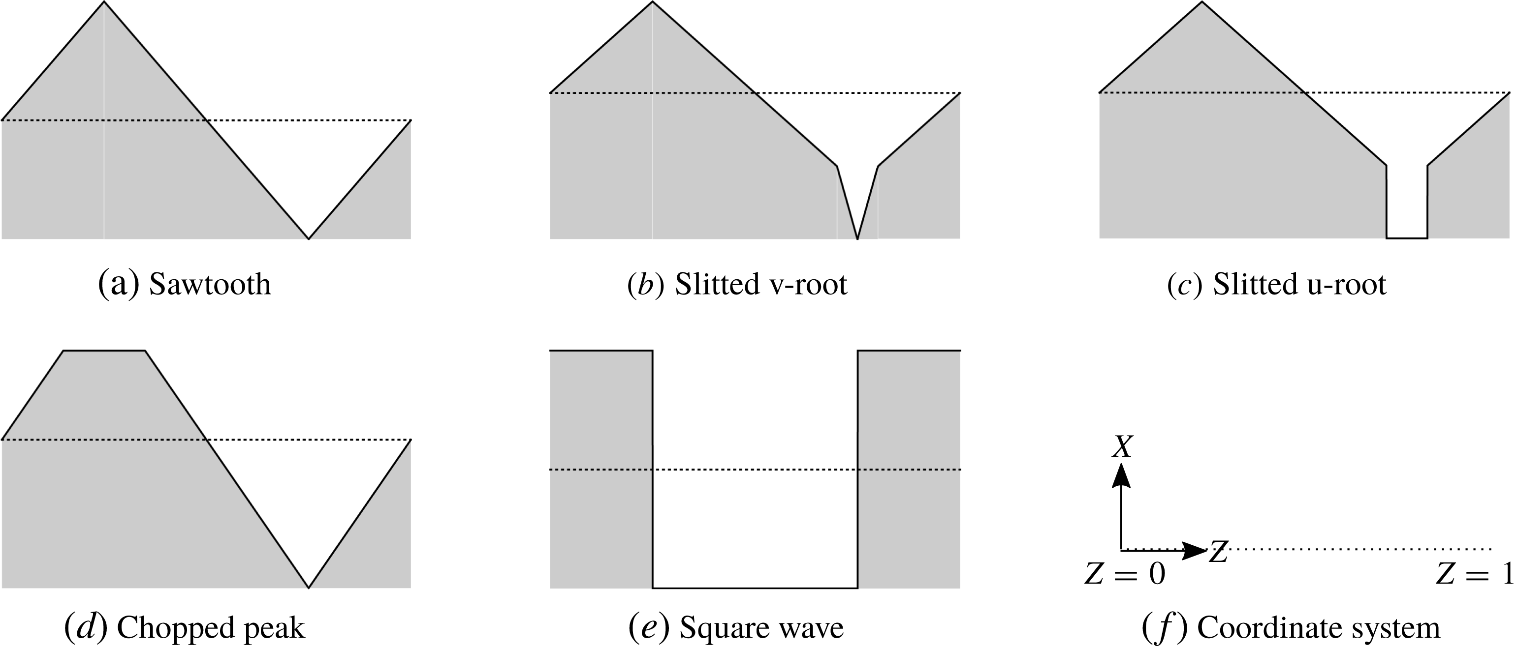
is a piecewise linear function, and we specifically focus on five different test cases: sawtooth serration, slitted v-root serration, slitted u-root serration, chopped peak serration and square wave. Our test-case geometries are depicted in figure 1, although the results are applicable to any piecewise linear or smooth, single-valued geometry. Note in all geometry cases, the
 $z=0,1$
boundaries of the periodic function are chosen to be away from any region of discontinuity of the edge. This ensures the solution captures any influence of the discontinuities.
Trailing-edge geometries. The shaded area denotes the rigid plate, with border
 $x=\tilde{c}F(z)$
, and the dotted line in each panel denotes
 $x=0$
.

In accordance with the model by Lyu et al. (Reference Lyu, Azarpeyvand and Sinayoko2016), the wall pressure gust has prescribed pressure
 $$\begin{eqnarray}p_{i}=P_{i}\text{e}^{\text{i}(k_{1}x+k_{3}z-\unicode[STIX]{x1D714}t)},\end{eqnarray}$$
where
 $P_{i}$
is the magnitude of the incident pressure,
 $\unicode[STIX]{x1D714}$
is the frequency, and
 $k_{1,3}$
are the wavenumbers in the streamwise and spanwise directions respectively. For simplicity, since the scattered solution depends linearly on the magnitude of the incident field, we set
 $P_{i}=1$
.
The scattered pressure,
 $p\text{e}^{-\text{i}\unicode[STIX]{x1D714}t}$
, satisfies the compressible convective Helmholtz equation,
 $$\begin{eqnarray}\unicode[STIX]{x1D6FD}^{2}\frac{\unicode[STIX]{x2202}^{2}p}{\unicode[STIX]{x2202}x^{2}}+\frac{\unicode[STIX]{x2202}^{2}p}{\unicode[STIX]{x2202}y^{2}}+\frac{\unicode[STIX]{x2202}^{2}p}{\unicode[STIX]{x2202}z^{2}}+2\text{i}kM\frac{\unicode[STIX]{x2202}p}{\unicode[STIX]{x2202}x}+k^{2}p=0,\end{eqnarray}$$
subject to boundary conditions of zero normal velocity on the rigid surface
 $$\begin{eqnarray}\left.\frac{\unicode[STIX]{x2202}p}{\unicode[STIX]{x2202}y}\right|_{y=0}=0\quad x<\tilde{c}F(z),\end{eqnarray}$$
and zero pressure jump across the wake downstream of the plate
 $$\begin{eqnarray}\unicode[STIX]{x0394}p|_{y=0}=-\text{e}^{\text{i}(k_{1}x+k_{3}z)}\quad x>\tilde{c}F(z),\end{eqnarray}$$
where
 $\unicode[STIX]{x0394}$
denotes the jump in value across
 $y=0_{+}$
and
 $y=0_{-}$
. Here
 $\unicode[STIX]{x1D6FD}^{2}=1-M^{2}$
and
 $k=\unicode[STIX]{x1D714}/c_{0}$
. We suppose the wake consists of a flat vortex sheet along
 $y=0$
,
 $x>\tilde{c}F(z)$
.
We finally impose a spanwise periodicity condition for the solution:
 $$\begin{eqnarray}p|_{z=1}=p|_{z=0}\text{e}^{\text{i}k_{3}},\quad \left.\frac{\unicode[STIX]{x2202}p}{\unicode[STIX]{x2202}z}\right|_{z=1}=\left.\frac{\unicode[STIX]{x2202}p}{\unicode[STIX]{x2202}z}\right|_{z=0}\text{e}^{\text{i}k_{3}}.\end{eqnarray}$$
To simplify the governing equation following Roger, Schram and De Santana (Reference Roger, Schram and De Santana2013) we use a convective transform,
 $$\begin{eqnarray}h=p(x,y,z)\text{e}^{\text{i}kMx/\unicode[STIX]{x1D6FD}^{2}}.\end{eqnarray}$$
This results in
 $$\begin{eqnarray}\displaystyle & \displaystyle \unicode[STIX]{x1D6FD}^{2}\frac{\unicode[STIX]{x2202}^{2}h}{\unicode[STIX]{x2202}x^{2}}+\frac{\unicode[STIX]{x2202}^{2}h}{\unicode[STIX]{x2202}y^{2}}+\frac{\unicode[STIX]{x2202}^{2}h}{\unicode[STIX]{x2202}z^{2}}+\left(\frac{k}{\unicode[STIX]{x1D6FD}}\right)^{2}h=0, & \displaystyle\end{eqnarray}$$
 $$\begin{eqnarray}\displaystyle & \displaystyle \left.\frac{\unicode[STIX]{x2202}h}{\unicode[STIX]{x2202}y}\right|_{y=0}=0\quad x<\tilde{c}F(z), & \displaystyle\end{eqnarray}$$
 $$\begin{eqnarray}\displaystyle & \displaystyle \unicode[STIX]{x0394}h|_{y=0}=-\text{e}^{\text{i}(\tilde{k}_{1}x+k_{3}z)}\quad x>\tilde{c}F(z) & \displaystyle\end{eqnarray}$$
 $$\begin{eqnarray}h|_{z=1}=h|_{z=0}\text{e}^{\text{i}k_{3}},\quad \left.\frac{\unicode[STIX]{x2202}h}{\unicode[STIX]{x2202}z}\right|_{z=1}=\left.\frac{\unicode[STIX]{x2202}h}{\unicode[STIX]{x2202}z}\right|_{z=0}\text{e}^{\text{i}k_{3}},\end{eqnarray}$$
 $\tilde{k_{1}}=k_{1}+kM\unicode[STIX]{x1D6FD}^{-2}$
.
We now use a non-orthogonal change of coordinates as done by Roger et al. (Reference Roger, Schram and De Santana2013) to make the boundary conditions more amenable to the Wiener–Hopf technique by removing the
 $z$
dependency of the half-regions on which the boundary conditions are prescribed (i.e. rather than have
 $x\gtrless \tilde{c}F(z)$
, have some
 $\unicode[STIX]{x1D709}\gtrless 0$
).
We choose the following variables:
 $$\begin{eqnarray}\displaystyle & \displaystyle \unicode[STIX]{x1D709}=\frac{x}{\unicode[STIX]{x1D6FD}}-cF(z), & \displaystyle\end{eqnarray}$$
 $$\begin{eqnarray}\displaystyle & \unicode[STIX]{x1D702}=y, & \displaystyle\end{eqnarray}$$
 $$\begin{eqnarray}\displaystyle & \unicode[STIX]{x1D701}=z, & \displaystyle\end{eqnarray}$$
 $c=\tilde{c}/\unicode[STIX]{x1D6FD}$
. This converts the governing equation and boundary conditions, equation (2.7), to
 $$\begin{eqnarray}\displaystyle & \displaystyle (1+c^{2}F^{\prime }(\unicode[STIX]{x1D701})^{2})\frac{\unicode[STIX]{x2202}^{2}h}{\unicode[STIX]{x2202}\unicode[STIX]{x1D709}^{2}}+\frac{\unicode[STIX]{x2202}^{2}h}{\unicode[STIX]{x2202}\unicode[STIX]{x1D702}^{2}}+\frac{\unicode[STIX]{x2202}^{2}h}{\unicode[STIX]{x2202}\unicode[STIX]{x1D701}^{2}}-2cF^{\prime }(\unicode[STIX]{x1D701})\frac{\unicode[STIX]{x2202}^{2}h}{\unicode[STIX]{x2202}\unicode[STIX]{x1D709}\unicode[STIX]{x2202}\unicode[STIX]{x1D701}}-cF^{\prime \prime }(\unicode[STIX]{x1D701})\frac{\unicode[STIX]{x2202}h}{\unicode[STIX]{x2202}\unicode[STIX]{x1D709}}+\left(\frac{k}{\unicode[STIX]{x1D6FD}}\right)^{2}h=0,\qquad & \displaystyle\end{eqnarray}$$
 $$\begin{eqnarray}\displaystyle & \displaystyle \left.\frac{\unicode[STIX]{x2202}h}{\unicode[STIX]{x2202}y}\right|_{\unicode[STIX]{x1D702}=0}=0\quad \unicode[STIX]{x1D709}<0,\qquad & \displaystyle\end{eqnarray}$$
 $$\begin{eqnarray}\displaystyle & \displaystyle \unicode[STIX]{x0394}h|_{\unicode[STIX]{x1D702}=0}=-\text{e}^{\text{i}\unicode[STIX]{x1D6FF}\unicode[STIX]{x1D709}+\text{i}\tilde{k}_{1}cF(\unicode[STIX]{x1D701})+\text{i}k_{3}\unicode[STIX]{x1D701}}\quad \unicode[STIX]{x1D709}>0,\qquad & \displaystyle\end{eqnarray}$$
 $$\begin{eqnarray}\displaystyle & h|_{\unicode[STIX]{x1D701}=1}=h|_{\unicode[STIX]{x1D701}=0}\text{e}^{\text{i}k_{3}}, & \displaystyle\end{eqnarray}$$
 $$\begin{eqnarray}\displaystyle & \displaystyle \left.\frac{\unicode[STIX]{x2202}h}{\unicode[STIX]{x2202}\unicode[STIX]{x1D701}}\right|_{\unicode[STIX]{x1D701}=1}=\left.\frac{\unicode[STIX]{x2202}h}{\unicode[STIX]{x2202}\unicode[STIX]{x1D701}}\right|_{\unicode[STIX]{x1D701}=0}\text{e}^{\text{i}k_{3}},\qquad & \displaystyle\end{eqnarray}$$
 $\unicode[STIX]{x1D6FF}=\tilde{k}_{1}\unicode[STIX]{x1D6FD}$
.
This completes the formulation of the mathematical model.
3 Analytic solution
We proceed to solve (2.9) by seeking a separable solution in the
 $\unicode[STIX]{x1D702}$
and
 $\unicode[STIX]{x1D701}$
coordinates. We note that in Roger et al. (Reference Roger, Schram and De Santana2013) the authors correctly identify that the physical space governing equation, (2.9) cannot be separated as the coefficients of the
 $\unicode[STIX]{x1D709}$
derivatives depend on
 $\unicode[STIX]{x1D701}$
. However, following Ayton & Kim (Reference Ayton and Kim2018) we see that in Fourier space (transforming the
 $\unicode[STIX]{x1D709}$
variable), the equation becomes separable.
We therefore first apply a Fourier transform in the
 $\unicode[STIX]{x1D709}$
variable,
 $$\begin{eqnarray}H(\unicode[STIX]{x1D706},\unicode[STIX]{x1D702},\unicode[STIX]{x1D701})=\int _{-\infty }^{\infty }h(\unicode[STIX]{x1D709},\unicode[STIX]{x1D702},\unicode[STIX]{x1D701})\text{e}^{\text{i}\unicode[STIX]{x1D706}\unicode[STIX]{x1D709}}\,\text{d}\unicode[STIX]{x1D709},\end{eqnarray}$$
then separate the solution into
 $\unicode[STIX]{x1D702}$
and
 $\unicode[STIX]{x1D701}$
dependencies,
 $H(\unicode[STIX]{x1D706},\unicode[STIX]{x1D702},\unicode[STIX]{x1D701})=Y(\unicode[STIX]{x1D706},\unicode[STIX]{x1D702})Z(\unicode[STIX]{x1D706},\unicode[STIX]{x1D701})$
, with separation constant
 $\unicode[STIX]{x1D712}$
. This results in equations
 $$\begin{eqnarray}Y^{\prime \prime }+\left(\left(\frac{k}{\unicode[STIX]{x1D6FD}}\right)^{2}-\unicode[STIX]{x1D706}^{2}-\unicode[STIX]{x1D712}^{2}\right)Y=0,\end{eqnarray}$$
and
 $$\begin{eqnarray}Z^{\prime \prime }+2\text{i}\unicode[STIX]{x1D706}cF^{\prime }Z^{\prime }+(\text{i}\unicode[STIX]{x1D706}cF^{\prime \prime }-\unicode[STIX]{x1D706}^{2}c^{2}(F^{\prime })^{2}+\unicode[STIX]{x1D712}^{2})Z=0.\end{eqnarray}$$
Equation (3.2) has solutions
 $$\begin{eqnarray}Y(\unicode[STIX]{x1D706},\unicode[STIX]{x1D702})=\text{sgn}(\unicode[STIX]{x1D702})\text{e}^{-|\unicode[STIX]{x1D702}|\sqrt{\unicode[STIX]{x1D706}^{2}-w^{2}}},\end{eqnarray}$$
where
 $$\begin{eqnarray}w^{2}=\left(\frac{k}{\unicode[STIX]{x1D6FD}}\right)^{2}-\unicode[STIX]{x1D712}^{2},\end{eqnarray}$$
and we have enforced a radiation condition as
 $y\rightarrow \infty$
.
Equation (3.3) has solutions
 $$\begin{eqnarray}Z(\unicode[STIX]{x1D706},\unicode[STIX]{x1D701})=\text{e}^{-\text{i}\unicode[STIX]{x1D706}cF(\unicode[STIX]{x1D701})}(A(\unicode[STIX]{x1D706})\cos (\unicode[STIX]{x1D712}\unicode[STIX]{x1D701})+B(\unicode[STIX]{x1D706})\sin (\unicode[STIX]{x1D712}\unicode[STIX]{x1D701})).\end{eqnarray}$$
We impose the periodicity boundary conditions to
 $Z$
to solve for
 $\unicode[STIX]{x1D712}$
and eliminate one of
 $A,B$
. This yields allowable modes,
 $$\begin{eqnarray}Z_{n}(\unicode[STIX]{x1D706},\unicode[STIX]{x1D701})=\text{e}^{-\text{i}\unicode[STIX]{x1D706}cF(\unicode[STIX]{x1D701})}\text{e}^{-\text{i}k_{3}\unicode[STIX]{x1D701}+2n\unicode[STIX]{x03C0}\text{i}\unicode[STIX]{x1D701}},\end{eqnarray}$$
and a general solution given by
 $$\begin{eqnarray}H(\unicode[STIX]{x1D706},\unicode[STIX]{x1D702},\unicode[STIX]{x1D701})=\mathop{\sum }_{n=-\infty }^{\infty }A_{n}(\unicode[STIX]{x1D706})\text{sgn}(\unicode[STIX]{x1D702})\text{e}^{-|\unicode[STIX]{x1D702}|\sqrt{\unicode[STIX]{x1D706}^{2}-w_{n}^{2}}}Z_{n}(\unicode[STIX]{x1D706},\unicode[STIX]{x1D701}),\end{eqnarray}$$
where
 $$\begin{eqnarray}w_{n}^{2}=\left(\frac{k}{\unicode[STIX]{x1D6FD}}\right)^{2}-\unicode[STIX]{x1D712}_{n}^{2},\quad \unicode[STIX]{x1D712}_{n}=\pm k_{3}+2n\unicode[STIX]{x03C0}.\end{eqnarray}$$
Importantly, rather than applying a Fourier series to deal with the
 $\unicode[STIX]{x1D701}$
variable, we have allowed for any permitted separable solution. This has shown specific spanwise modes are a direct result of the governing equation.
Now we have an expression for the Fourier transform of the solution, (3.8), we can use the
 $\unicode[STIX]{x1D702}$
boundary conditions, (2.9b
) and (2.9c
), and apply the Wiener–Hopf technique to solve for
 $A_{n}(\unicode[STIX]{x1D706})$
.
First we transform (2.9b ) to obtain
 $$\begin{eqnarray}-\mathop{\sum }_{n=-\infty }^{\infty }A_{n}(\unicode[STIX]{x1D706})\sqrt{\unicode[STIX]{x1D706}^{2}-w_{n}^{2}}Z_{n}(\unicode[STIX]{x1D706},\unicode[STIX]{x1D701})=U_{+}(\unicode[STIX]{x1D706},\unicode[STIX]{x1D701}),\end{eqnarray}$$
where a subscript
 $+$
denotes a function that is analytic in the upper half
 $\unicode[STIX]{x1D706}$
-plane. Aside from its region of analyticity, the function
 $U_{+}$
is formally unknown.
Second we transform (2.9c ) to obtain
 $$\begin{eqnarray}2\mathop{\sum }_{n=-\infty }^{\infty }A_{n}(\unicode[STIX]{x1D706})Z_{n}(\unicode[STIX]{x1D706},\unicode[STIX]{x1D701})=U_{-}(\unicode[STIX]{x1D706},\unicode[STIX]{x1D701})+\left(\frac{\text{e}^{\text{i}\tilde{k}_{1}cF(\unicode[STIX]{x1D701})+\text{i}k_{3}\unicode[STIX]{x1D701}}}{\text{i}(\unicode[STIX]{x1D706}+\unicode[STIX]{x1D6FF})}\right)_{+},\end{eqnarray}$$
where a subscript
 $-$
denotes a function that is analytic in the lower half
 $\unicode[STIX]{x1D706}$
-plane. Aside from its region of analyticity, the function
 $U_{-}$
is formally unknown.
Since the
 $Z_{n}$
are a complete orthogonal basis we can expand the right-hand sides of (3.10) and (3.11) in terms of this basis. Furthermore the
 $Z_{n}$
are entire functions of
 $\unicode[STIX]{x1D706}$
thus do not affect the domains of analyticity of any functions. We therefore write
 $$\begin{eqnarray}\displaystyle & \displaystyle U_{\pm }(\unicode[STIX]{x1D706},\unicode[STIX]{x1D701})=\mathop{\sum }_{n=-\infty }^{\infty }U_{\pm }^{n}(\unicode[STIX]{x1D706})Z_{n}(\unicode[STIX]{x1D706},\unicode[STIX]{x1D701}), & \displaystyle\end{eqnarray}$$
 $$\begin{eqnarray}\displaystyle & \displaystyle \left(\frac{\text{e}^{\text{i}\tilde{k}_{1}cF(\unicode[STIX]{x1D701})+\text{i}k_{3}\unicode[STIX]{x1D701}}}{\text{i}(\unicode[STIX]{x1D706}+\unicode[STIX]{x1D6FF})}\right)_{+}=\left(\frac{1}{\text{i}(\unicode[STIX]{x1D706}+\unicode[STIX]{x1D6FF})}\right)_{+}\mathop{\sum }_{n=-\infty }^{\infty }E_{n}(\unicode[STIX]{x1D706})Z_{n}(\unicode[STIX]{x1D706},\unicode[STIX]{x1D701}). & \displaystyle\end{eqnarray}$$
 $U_{\pm }^{n}$
are unknown functions which are analytic in the upper/lower half-plane, whereas the
 $E_{n}$
are known entire functions that can be determined via
 $$\begin{eqnarray}E_{n}(\unicode[STIX]{x1D706})=\int _{0}^{1}\text{e}^{\text{i}\tilde{k}_{1}cF(\unicode[STIX]{x1D701})+\text{i}k_{3}\unicode[STIX]{x1D701}}\bar{Z}_{n}(\bar{\unicode[STIX]{x1D706}},\unicode[STIX]{x1D701})\,\text{d}\unicode[STIX]{x1D701}.\end{eqnarray}$$
We use orthogonality of the
 $Z_{n}$
to consider each mode separately, and combine (3.10) and (3.11) to form a single Wiener–Hopf equation for the
 $n$
th mode:
 $$\begin{eqnarray}2\left(A_{n}(\unicode[STIX]{x1D706})\sqrt{\unicode[STIX]{x1D706}-w_{n}}\right)_{+}=\left(U_{-}^{n}(\unicode[STIX]{x1D706})\sqrt{\unicode[STIX]{x1D706}-w_{n}}\right)_{-}+\frac{E_{n}(\unicode[STIX]{x1D706})(\sqrt{\unicode[STIX]{x1D706}-w_{n}})_{-}}{\text{i}(\unicode[STIX]{x1D706}+\unicode[STIX]{x1D6FF})_{+}}.\end{eqnarray}$$
We additively factorise the final term on the right-hand side to give
 $$\begin{eqnarray}\displaystyle & & \displaystyle 2\left(A_{n}(\unicode[STIX]{x1D706})\sqrt{\unicode[STIX]{x1D706}-w_{n}}\right)_{+}=\left(U_{-}^{n}(\unicode[STIX]{x1D706})\sqrt{\unicode[STIX]{x1D706}-w_{n}}\right)_{-}\nonumber\\ \displaystyle & & \displaystyle \quad +\,E_{n}(\unicode[STIX]{x1D706})\left(\left[\frac{(\sqrt{\unicode[STIX]{x1D706}-w_{n}})_{-}}{\text{i}(\unicode[STIX]{x1D706}+\unicode[STIX]{x1D6FF})_{+}}-\frac{(\sqrt{-\unicode[STIX]{x1D6FF}-w_{n}})_{-}}{\text{i}(\unicode[STIX]{x1D706}+\unicode[STIX]{x1D6FF})_{+}}\right]_{-}+\left[\frac{(\sqrt{-\unicode[STIX]{x1D6FF}-w_{n}})_{-}}{\text{i}(\unicode[STIX]{x1D706}+\unicode[STIX]{x1D6FF})_{+}}\right]_{+}\right),\qquad\end{eqnarray}$$
which is decomposed into functions which are analytic in the upper and lower half-planes. To complete the Wiener–Hopf method, we must apply Liouville’s theorem to determine an entire function which both
 $+$
and
 $-$
contributions to (3.15) equal (by analytic continuation).
To enable the use of Liouville’s theorem in the Wiener–Hopf method we must consider the large
 $\unicode[STIX]{x1D706}$
behaviour of each term in (3.14). Large
 $\unicode[STIX]{x1D706}$
corresponds to small
 $x$
through inverting the Fourier transform, therefore we consider the physical possibilities for
 $A_{n}(\unicode[STIX]{x1D706})\sqrt{\unicode[STIX]{x1D706}^{2}-w_{n}^{2}}$
and
 $U_{-}^{n}(\unicode[STIX]{x1D706})$
, which are modal coefficients of the scattered normal velocity just above the wake (
 $x>0$
), and the scattered pressure jump across the surface of the plate (
 $x<0$
) respectively.
First we consider the spanwise dependency of these functions and the
 $\unicode[STIX]{x1D706}$
dependencies arising from the
 $Z_{n}$
basis expansion, as done by Envia (Reference Envia1988). We know the physical spanwise dependency of the scattered pressure jump just downstream of the trailing edge is
 ${\sim}\text{e}^{\text{i}\tilde{k}_{1}cF(\unicode[STIX]{x1D701})+\text{i}k_{3}\unicode[STIX]{x1D701}}$
. By linearity the spanwise dependency of the pressure just upstream of the trailing edge and the velocity just downstream of the trailing edge must be identical. Therefore, upon expanding the unknown Fourier transforms of the scattered pressure jump and normal velocity in the
 $Z_{n}$
basis we must obtain factors of
 $E_{n}(\unicode[STIX]{x1D706})$
in
 $A_{n}(\unicode[STIX]{x1D706})$
and
 $U_{-}^{n}(\unicode[STIX]{x1D706})$
corresponding to the expansion of their
 $\unicode[STIX]{x1D701}$
dependencies. In (3.14) we therefore factor out
 $E_{n}(\unicode[STIX]{x1D706})$
by writing
 $A_{n}(\unicode[STIX]{x1D706})=\tilde{A}_{n}(\unicode[STIX]{x1D706})E_{n}(\unicode[STIX]{x1D706})$
and
 $U_{-}^{n}(\unicode[STIX]{x1D706})=\tilde{U} _{-}^{n}(\unicode[STIX]{x1D706})E_{n}(\unicode[STIX]{x1D706})$
.
Both
 $\tilde{A}_{n}(\unicode[STIX]{x1D706})$
and
 $\tilde{U} _{-}^{n}(\unicode[STIX]{x1D706})$
could still contain unknown functions of
 $\unicode[STIX]{x1D706}$
due to streamwise dependencies. To consider the streamwise dependencies we use the unsteady Kutta condition which enforces that the pressure is not singular on approach to the trailing edge
 $x\rightarrow 0$
, therefore
 $\tilde{A}_{n}(\unicode[STIX]{x1D706})\sqrt{\unicode[STIX]{x1D706}^{2}-w_{n}^{2}}\sim \unicode[STIX]{x1D706}^{-1/2}$
and
 $\tilde{U} _{-}^{n}(\unicode[STIX]{x1D706})\sim \unicode[STIX]{x1D706}^{-1}$
as
 $\unicode[STIX]{x1D706}\rightarrow \infty$
.
We therefore see both the
 $+$
and
 $-$
contributions to (3.15), after factorisation of
 $E_{n}$
, decay to zero for large
 $\unicode[STIX]{x1D706}$
, thus the entire function they equate to must be zero. We take the
 $+$
functions from (3.15) to solve for
 $A_{n}$
, yielding
 $$\begin{eqnarray}A_{n}(\unicode[STIX]{x1D706})=\frac{E_{n}(\unicode[STIX]{x1D706})\sqrt{-\unicode[STIX]{x1D6FF}-w_{n}}}{2\text{i}(\unicode[STIX]{x1D706}+\unicode[STIX]{x1D6FF})\sqrt{\unicode[STIX]{x1D706}-w_{n}}}.\end{eqnarray}$$
This gives
 $$\begin{eqnarray}H(\unicode[STIX]{x1D706},\unicode[STIX]{x1D702},\unicode[STIX]{x1D701})=\mathop{\sum }_{n=-\infty }^{\infty }\frac{E_{n}(\unicode[STIX]{x1D706})\sqrt{-\unicode[STIX]{x1D6FF}-w_{n}}}{2\text{i}(\unicode[STIX]{x1D706}+\unicode[STIX]{x1D6FF})\sqrt{\unicode[STIX]{x1D706}-w_{n}}}\text{sgn}(\unicode[STIX]{x1D702})\text{e}^{-|\unicode[STIX]{x1D702}|\sqrt{\unicode[STIX]{x1D706}^{2}-w_{n}^{2}}}Z_{n}(\unicode[STIX]{x1D706},\unicode[STIX]{x1D701}).\end{eqnarray}$$
We invert the Fourier transform and apply the method of steepest descents to obtain a far-field (
 $r\gg 1$
) approximation as
 $$\begin{eqnarray}h(r,\unicode[STIX]{x1D703},z)\sim \mathop{\sum }_{n=-\infty }^{\infty }\frac{E_{n}(-w_{n}\cos \unicode[STIX]{x1D703})\sqrt{-\unicode[STIX]{x1D6FF}-w_{n}}}{2\text{i}(\unicode[STIX]{x1D6FF}-w_{n}\cos \unicode[STIX]{x1D703})}Z_{n}(-w_{n}\cos \unicode[STIX]{x1D703},z)\sin \left(\frac{\unicode[STIX]{x1D703}}{2}\right)\frac{\text{e}^{\text{i}w_{n}r}\text{e}^{\text{i}\unicode[STIX]{x03C0}/4}}{\sqrt{\unicode[STIX]{x03C0}r}}\text{e}^{\text{i}w_{n}\cos \unicode[STIX]{x1D703}\,cF(z)},\end{eqnarray}$$
where
 $(r,\unicode[STIX]{x1D703},z)$
are cylindrical polar coordinates centred on
 $x=y=0$
. We note for sufficiently large
 $n$
(dependent on the variables in this study) the scattered modes are cut-off i.e.
 $\text{Im}(w_{n})>0$
, therefore in practice one only has to sum a finite number of terms in (3.18) to calculate the far-field pressure.
This completes our analytic solution for a general trailing-edge geometry,
 $F(z)$
.
3.1 Limit as
 $c\rightarrow 0$

We can take our general solution, (3.18), and limit
 $c\rightarrow 0$
to validate it with the straight-edged case whose result features in Noble (Reference Noble1958) for
 $k_{3}=0$
.
In this case as
 $c\rightarrow 0$
,
 $E_{m}\rightarrow 0$
for
 $m\geqslant 1$
and
 $E_{0}\rightarrow 1$
. This yields a limit,
 $h_{0}(r,\unicode[STIX]{x1D703},z)=\lim _{c\rightarrow 0}h(r,\unicode[STIX]{x1D703},z)$
of
 $$\begin{eqnarray}h_{0}(r,\unicode[STIX]{x1D703},z)=\frac{\sqrt{-\unicode[STIX]{x1D6FF}-w_{0}}}{2\text{i}(\unicode[STIX]{x1D6FF}-w_{0}\cos \unicode[STIX]{x1D703})}\sin \left(\frac{\unicode[STIX]{x1D703}}{2}\right)\frac{\text{e}^{\text{i}w_{0}r}\text{e}^{\text{i}\unicode[STIX]{x03C0}/4}}{\sqrt{\unicode[STIX]{x03C0}r}}.\end{eqnarray}$$
The corresponding limit of the Fourier transform of this solution (equivalent to (3.17) under the limit
 $c\rightarrow 0$
) is
 $$\begin{eqnarray}H_{0}(\unicode[STIX]{x1D706},\unicode[STIX]{x1D702},\unicode[STIX]{x1D701})=\frac{\sqrt{-\unicode[STIX]{x1D6FF}-w_{0}}}{2\text{i}(\unicode[STIX]{x1D706}+\unicode[STIX]{x1D6FF})\sqrt{\unicode[STIX]{x1D706}-w_{0}}}\text{sgn}(\unicode[STIX]{x1D702})\text{e}^{-|\unicode[STIX]{x1D702}|\sqrt{\unicode[STIX]{x1D706}^{2}-w_{0}^{2}}}.\end{eqnarray}$$
This is in agreement with the solution for a straight trailing edge as can be seen by comparing with the half-plate scattering problem in Noble (Reference Noble1958, § 2).
Thus our solution for the general trailing-edge geometry is in agreement with the straight-edged result when
 $c\rightarrow 0$
.
4 Results
We now present results calculated from the analytic expression (3.18). In all cases, all propagating modes are included in the summation whilst all cut-off modes are excluded. We shall restrict ourselves to low Mach numbers
 $M<0.4$
as this is the range used in typical experimental tests, although higher (subsonic) Mach numbers are permitted in this analytic formulation.
4.1 Comparison with Lyu et al. (Reference Lyu, Azarpeyvand and Sinayoko2016)
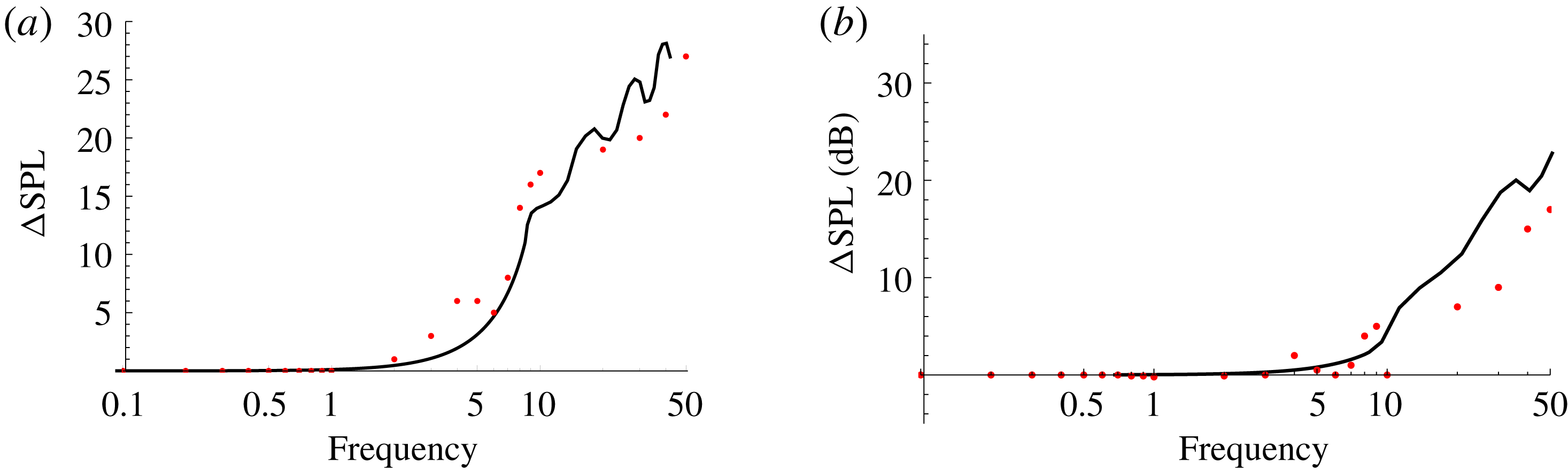
We have previously shown in § 3.1 that our new solution is in agreement with the straight-edged formulation. We now validate our new method for a serrated trailing-edge geometry by comparing our far-field results against those from Lyu et al. (Reference Lyu, Azarpeyvand and Sinayoko2016) which have been compared to a finite element solution. In particular we compare the reduction in far-field sound pressure level (SPL), denoted as
 $\unicode[STIX]{x0394}\text{SPL}$
, at
 $90^{\circ }$
above a sawtooth serrated trailing edge (compared to a straight edge) at the mid-span of the serration,
 $z=0.5$
, with
 $k_{3}=0$
, as illustrated in figure 5 from Lyu et al. (Reference Lyu, Azarpeyvand and Sinayoko2016). The SPL defined in that paper is
 $$\begin{eqnarray}\text{SPL}=20\log _{10}|h|,\end{eqnarray}$$
where
 $h$
is the far-field pressure (denoted as
 $p_{f}$
in Lyu et al.
Reference Lyu, Azarpeyvand and Sinayoko2016), which from our analysis will come from (3.18) evaluated at a suitably large value of
 $r$
(chosen to be
 $r=10$
). We also choose
 $k=0.7Mk_{1}$
as done in Lyu et al. (Reference Lyu, Azarpeyvand and Sinayoko2016), since it is claimed by Chase (Reference Chase1987) that the convection velocity,
 $U_{c}$
, of the wall pressure gust is typically satisfied by
 $U_{c}\approx 0.7U$
, where
 $U$
is the uniform mean flow velocity.
Reduction of far-field SPL (
 $\unicode[STIX]{x0394}\text{SPL}$
) for a serrated edge plotted against non-dimensionalised frequency. Results taken from Lyu et al. (Reference Lyu, Azarpeyvand and Sinayoko2016) are plotted as red circles. Finite chord length to serration wavelength,
 $\unicode[STIX]{x1D706}$
, given for Lyu et al.’s (Reference Lyu, Azarpeyvand and Sinayoko2016) results. (a)
 $M=0.1$
,
 $c=4/3$
,
 $\unicode[STIX]{x1D706}/(\text{chord length})=0.15$
; (b)
 $M=0.2$
,
 $c=40/3$
,
 $\unicode[STIX]{x1D706}/(\text{chord length})=0.03$
.

We illustrate the good comparison between our new method and Lyu et al.’s (Reference Lyu, Azarpeyvand and Sinayoko2016) method in figure 2 for both shallow (
 $c$
small) and sharp (
 $c$
large) serrations. Note the results in Lyu et al. (Reference Lyu, Azarpeyvand and Sinayoko2016) use a finite chord length to non-dimensionalise frequency, whilst we use the serration wavelength,
 $\unicode[STIX]{x1D706}$
. The finite chord of Lyu et al. (Reference Lyu, Azarpeyvand and Sinayoko2016) ensures a rescattering of the trailing-edge field by the leading edge (as discussed by Roger & Moreau (Reference Roger and Moreau2005, Reference Roger and Moreau2009)) is captured by the far-field results, whereas our results do not account for this. We therefore expect small variations between our results and attribute them to this additional scattering. Additionally Lyu’s solution is an iterative solution, truncated at the second iteration. This is stated to have errors of
 ${\sim}2$
dB compared to the first iteration, however it is unclear what further errors exist between the second and higher iterations. By truncating the solution at the second iteration, higher-order modes are neglected in Lyu et al. (Reference Lyu, Azarpeyvand and Sinayoko2016). The solution presented in this paper does not require truncation of higher-order modes; all propagating modes are accounted for in the far-field solution.
4.2 SPL for different trailing-edge geometries
In this section we present results for the far-field sound given by (4.1) for the five different test-case trailing-edge geometries shown in figure 1. We label each geometry (a)–(e) as S, SV, SU, CP, SQ respectively.
Specifically the geometries are given by
 $$\begin{eqnarray}\displaystyle & \displaystyle \text{sawtooth}\quad F_{S}(z)=\left\{\begin{array}{@{}ll@{}}z,\quad & z\in \left[0,{\textstyle \frac{1}{4}}\right),\\ {\textstyle \frac{1}{2}}-z,\quad & z\in \left({\textstyle \frac{1}{4}},{\textstyle \frac{3}{4}}\right),\\ z-1,\quad & z\in \left({\textstyle \frac{3}{4}},1\right],\end{array}\right. & \displaystyle\end{eqnarray}$$
 $$\begin{eqnarray}\displaystyle & \displaystyle \text{slitted v\text{-}root}\quad F_{SV}(z)=\left\{\begin{array}{@{}ll@{}}{\textstyle \frac{2}{3}}z,\quad & z\in \left[0,{\textstyle \frac{1}{4}}\right),\\ {\textstyle \frac{2}{3}}\left({\textstyle \frac{1}{2}}-z\right),\quad & z\in \left({\textstyle \frac{1}{4}},{\textstyle \frac{7}{10}}\right),\\ {\textstyle \frac{8}{3}}-4z,\quad & z\in \left({\textstyle \frac{7}{10}},{\textstyle \frac{3}{4}}\right),\\ -{\textstyle \frac{10}{3}}+4z,\quad & z\in \left({\textstyle \frac{3}{4}},{\textstyle \frac{4}{5}}\right),\\ {\textstyle \frac{2}{3}}(z-1),\quad & z\in \left({\textstyle \frac{4}{5}},1\right],\end{array}\right. & \displaystyle\end{eqnarray}$$
 $$\begin{eqnarray}\displaystyle & \displaystyle \text{slitted u\text{-}root}\quad F_{SU}(z)=\left\{\begin{array}{@{}ll@{}}{\textstyle \frac{2}{3}}z,\quad & z\in \left[0,{\textstyle \frac{1}{4}}\right),\\ {\textstyle \frac{2}{3}}\left({\textstyle \frac{1}{2}}-z\right),\quad & z\in \left({\textstyle \frac{1}{4}},{\textstyle \frac{7}{10}}\right),\\ -{\textstyle \frac{1}{3}},\quad & z\in \left({\textstyle \frac{7}{10}},{\textstyle \frac{4}{5}}\right),\\ {\textstyle \frac{2}{3}}(z-1),\quad & z\in \left({\textstyle \frac{4}{5}},1\right],\end{array}\right. & \displaystyle\end{eqnarray}$$
 $$\begin{eqnarray}\displaystyle & \displaystyle \text{chopped peak}\quad F_{CP}(z)={\textstyle \frac{5}{4}}\left\{\begin{array}{@{}ll@{}}z,\quad & z\in \left[0,{\textstyle \frac{3}{20}}\right),\\ {\textstyle \frac{3}{20}},\quad & z\in \left({\textstyle \frac{3}{20}},{\textstyle \frac{7}{20}}\right),\\ {\textstyle \frac{1}{2}}-z,\quad & z\in \left({\textstyle \frac{7}{20}},{\textstyle \frac{3}{4}}\right),\\ z-1,\quad & z\in \left(\frac{3}{4},1\right],\end{array}\right. & \displaystyle\end{eqnarray}$$
 $$\begin{eqnarray}\displaystyle & \displaystyle \text{square wave}\quad F_{SQ}(z)={\textstyle \frac{1}{4}}\left\{\begin{array}{@{}ll@{}}1,\quad & z\in \left[0,{\textstyle \frac{1}{4}}\right),\\ -1,\quad & z\in \left({\textstyle \frac{1}{4}},{\textstyle \frac{3}{4}}\right),\\ 1,\quad & z\in \left({\textstyle \frac{3}{4}},1\right].\end{array}\right. & \displaystyle\end{eqnarray}$$
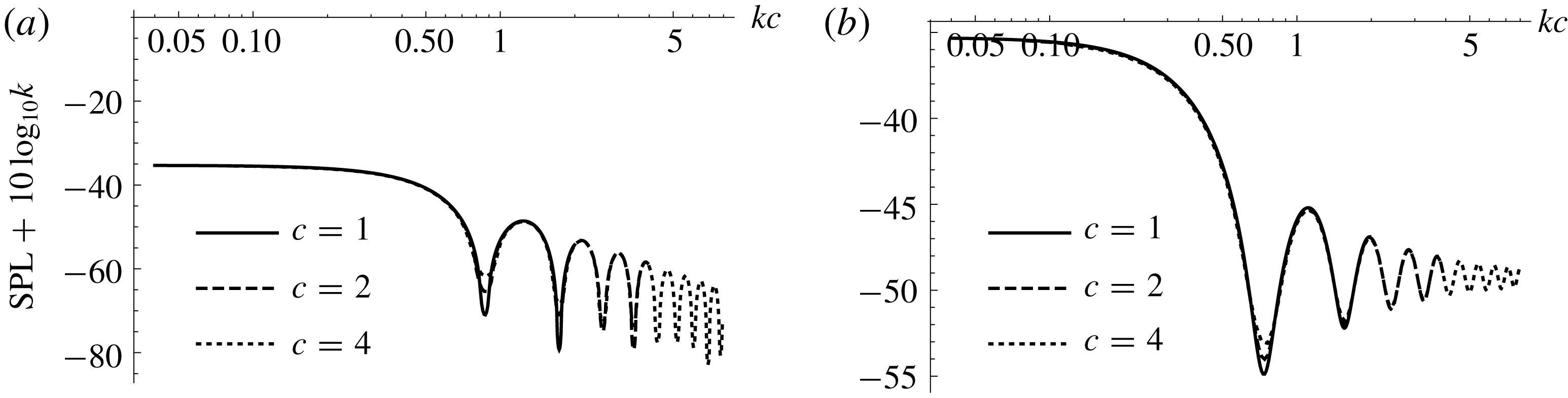
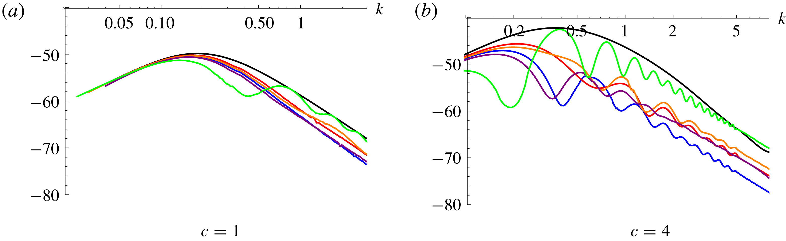
First we note a collapse of the results through a suitable scaling of
 $k$
and SPL as shown in figure 3; therefore we shall consider results from here as functions of scaled frequency
 $kc$
.
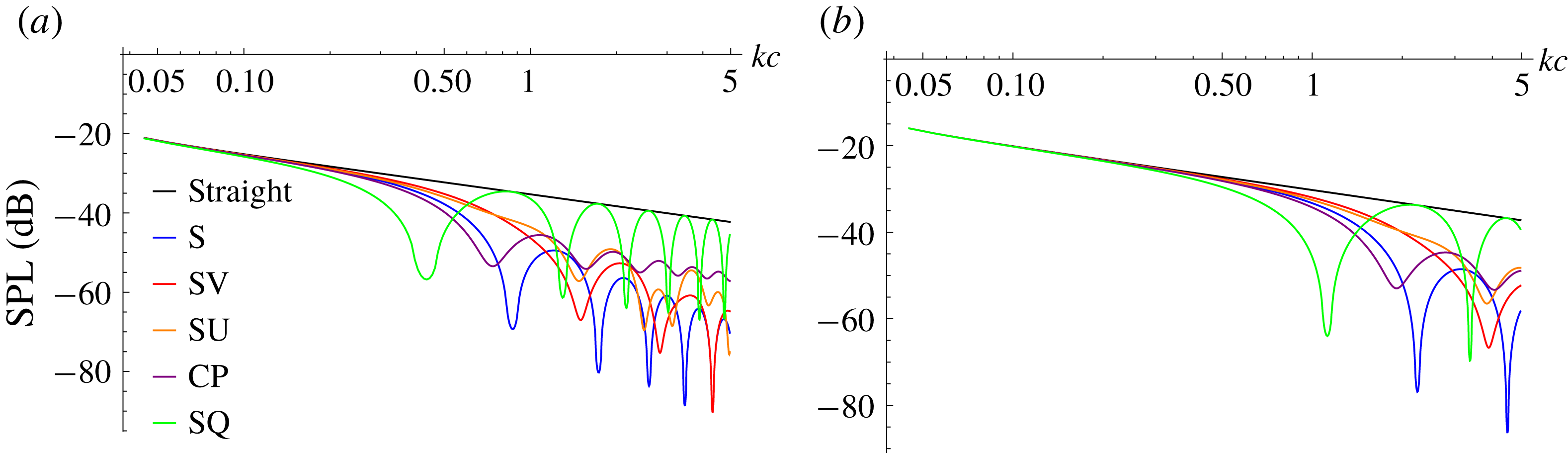
We plot SPL against scaled frequency for the five different trailing-edge geometries in figure 4 for different flow speeds. Whilst this does not indicate the reduction of noise for a realistic flow over a serrated trailing edge (as we have restricted to
 $k_{3}=0$
only) it provides us a foundation on which to understand the key influential parameters in the analytic solution and how they affect the far-field noise.
Scaled pressure spectra with scaled frequency for two different trailing-edge geometries, at
 $M=0.1$
, with
 $k_{3}=0$
. (a) Serration (S); (b) chopped peak (CP).

Pressure spectra for trailing-edge geometries (a) to (e), with
 $k_{3}=0$
. (a)
 $M=0.1$
(a); (b)
 $M=0.3$
.

It is clear from figure 4 that different trailing-edge geometries are best at reducing scattered noise at different mid-range frequencies; however, at high frequencies the sawtooth (S) and serrated v-root (SV) seem preferential over the other geometries. This variation in optimal SPL reduction occurs because every SPL for a non-straight edge exhibits oscillatory behaviour as
 $kc$
increases. This indicates an interference effect in the far field; in particular, where there are minima of the spectra there is a strong destructive interference between acoustic fields scattered at the tip and at the root of each geometry. The chopped peak (CP) exhibits the weakest oscillation (smallest amplitude variation in the oscillations) indicating there is weaker tip and root interference, whilst the square wave (SQ) has the greatest oscillation indicating a strong tip and root interference. The interference is clearly dependent on the flow speed,
 $M$
, and the specific trailing-edge geometry as all oscillations vary as we change these parameters.
The modal expansion coefficients,
 $E_{n}(-w_{n}\cos \unicode[STIX]{x1D703})$
found in (3.18), are key to understanding the tip and root interference. We illustrate this by considering
 $E_{0}(-w_{0}\cos \unicode[STIX]{x1D703})$
(the zeroth modal coefficient) for each geometry at
 $\unicode[STIX]{x1D703}=90^{\circ }$
and
 $k_{3}=0$
. These coefficients are calculated from (3.13) and given by
 $$\begin{eqnarray}\displaystyle & \displaystyle E_{0}^{S}(s)=\frac{1}{s}\sin (s), & \displaystyle\end{eqnarray}$$
 $$\begin{eqnarray}\displaystyle & \displaystyle E_{0}^{SV}(s)=\frac{\text{i}\text{e}^{-\text{i}s/3}}{2s}(1+5\text{e}^{\text{i}s/5}-6\text{e}^{\text{i}s/2}), & \displaystyle\end{eqnarray}$$
 $$\begin{eqnarray}\displaystyle & \displaystyle E_{0}^{SU}(s)=\frac{\text{e}^{-\text{i}s/3}}{10s}(s-30\text{i}\text{e}^{\text{i}s/5}(\text{e}^{3\text{i}s/10}-1)), & \displaystyle\end{eqnarray}$$
 $$\begin{eqnarray}\displaystyle & \displaystyle E_{0}^{CP}(s)=\frac{\text{e}^{-5\text{i}s/16}}{5s}(s\text{e}^{\text{i}s/2}-8\text{i}(\text{e}^{\text{i}s/2}-1)), & \displaystyle\end{eqnarray}$$
 $$\begin{eqnarray}\displaystyle & \displaystyle E_{0}^{SQ}(s)=\cos \left(\frac{s}{4}\right), & \displaystyle\end{eqnarray}$$
 $s=\unicode[STIX]{x1D6FF}c/\unicode[STIX]{x1D6FD}$
.
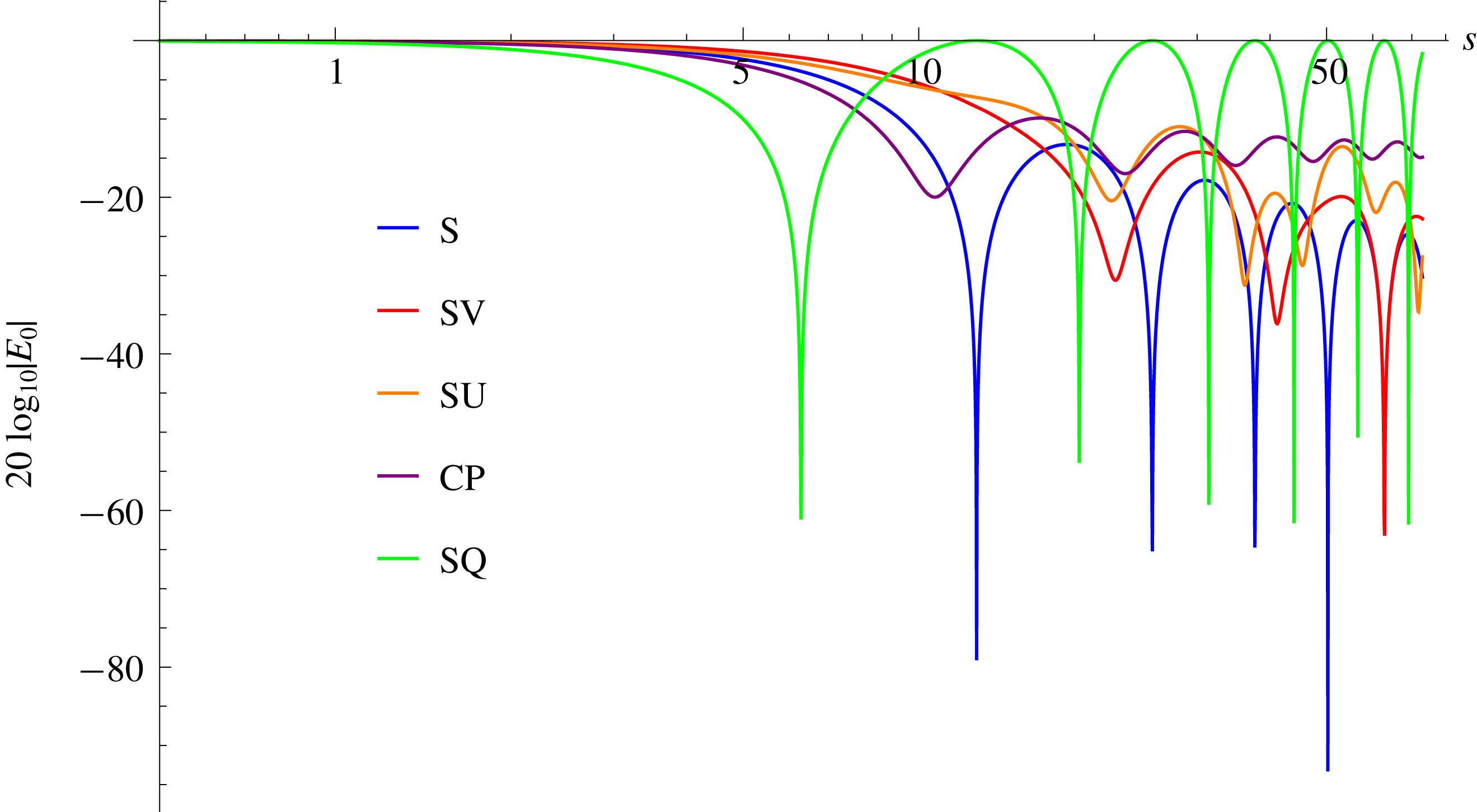
In figure 5 we plot
 $20\log _{10}|E_{0}(s)|$
for each of the edge geometries and compare to figure 4(a). We see the oscillations given by these
 $E_{0}$
functions very closely match the oscillations of the full SPL. We also see the relative magnitudes of the
 $E_{0}$
functions match the full SPL. The relative behaviour of the SPL is therefore dominated by the zeroth modal expansion term,
 $E_{0}$
. Higher-order modes have an effect once they are cut-on: this requires
 $k\unicode[STIX]{x1D6FD}^{-1}-2n\unicode[STIX]{x03C0}>0$
for the
 $n$
th mode to be cut-on.
Value of
 $20\log _{10}|E_{0}(s)|$
, for
 $k_{3}=0$
, for trailing-edge geometries (a) to (e).

The
 $E_{0}$
modal coefficients therefore provide us with a very simple formulation for the expected interference of the root and tip, as these coefficients can be calculated from (3.13) without any need for the Wiener–Hopf method. The coefficients also indicate, when
 $k_{3}=0$
, why for large
 $kc$
values the sawtooth (S) and serrated v-root (SV) are better at reducing noise than the other geometries. If we consider the large
 $s$
(corresponding to large
 $kc$
) behaviour of (4.3), we see that the sawtooth and serrated v-root coefficients behave as
 $O(s^{-1})$
, whilst the remaining geometries behave as
 $O(1)$
. Therefore we expect for increasingly sharp serrations, the sawtooth and serrated v-root reduce noise compared to the straight edge as
 ${\sim}\log (kc)$
; however, the other geometries (the serrated u-root, chopped peak and square wave) will tend to a constant noise reduction.
To ensure this conclusion still holds when higher modes are cut-on, we consider the higher modal coefficients
 $E_{n}$
. For simplicity we illustrate the behaviour with the sawtooth coefficients,
 $E_{n}^{S}(-w_{n}\cos \unicode[STIX]{x1D703})$
, and the square wave coefficients,
 $E_{n}^{SQ}(-w_{n}\cos \unicode[STIX]{x1D703})$
, as these are indicative of the two different cases which can occur. We again evaluate these at
 $\unicode[STIX]{x1D703}=90^{\circ }$
and
 $k_{3}=0$
; therefore
 $E_{n}$
for these two geometries are given by
 $$\begin{eqnarray}\displaystyle & \displaystyle E_{n}^{S}(s)=\frac{-4s\text{e}^{-\text{i}n\unicode[STIX]{x03C0}}}{4n^{2}\unicode[STIX]{x03C0}^{2}-s^{2}}\sin \left(\frac{1}{4}(2n\unicode[STIX]{x03C0}+s)\right), & \displaystyle\end{eqnarray}$$
 $$\begin{eqnarray}\displaystyle & \displaystyle E_{n}^{SQ}(s)=\left\{\begin{array}{@{}ll@{}}{\displaystyle \frac{\text{i}\text{e}^{\text{i}(n-1)\unicode[STIX]{x03C0}/2}}{n\unicode[STIX]{x03C0}}}\sin \left({\displaystyle \frac{s}{4}}\right)\quad & n~\text{odd},\\ 0\quad & n~\text{even}.\end{array}\right. & \displaystyle\end{eqnarray}$$
For large
 $s$
, the
 $n$
th mode coefficients behave similarly to the zeroth mode coefficients, with the exception that for the mode
 $n\approx s/2\unicode[STIX]{x03C0}$
,
 $E_{n}^{S}(s)\sim -1/2$
. Our conclusion, therefore, of the sawtooth and serrated v-root experiencing a reduction of noise as
 ${\sim}\log (kc)$
for increasing
 $kc$
, still holds, and we predict these geometries are preferential for large
 $kc$
values even when higher modes contribute. The emergence of a large
 $n$
mode whose coefficient does not decay with
 $kc$
suggests there is a redistribution of the acoustic energy from lower cut-on modes to these higher cut-off modes as the serration is sharpened (as
 $c$
increases).
4.3 Far-field directivity
Here we consider the effect of varying
 $\unicode[STIX]{x1D703}$
on the far-field SPL by plotting the directivity patterns (defined as SPL plotted as a function of observer angle
 $\unicode[STIX]{x1D703}$
). It is known that SPL varies as observer angle
 $\unicode[STIX]{x1D703}$
varies, more so with higher frequency interactions (Lyu et al.
Reference Lyu, Azarpeyvand and Sinayoko2016).
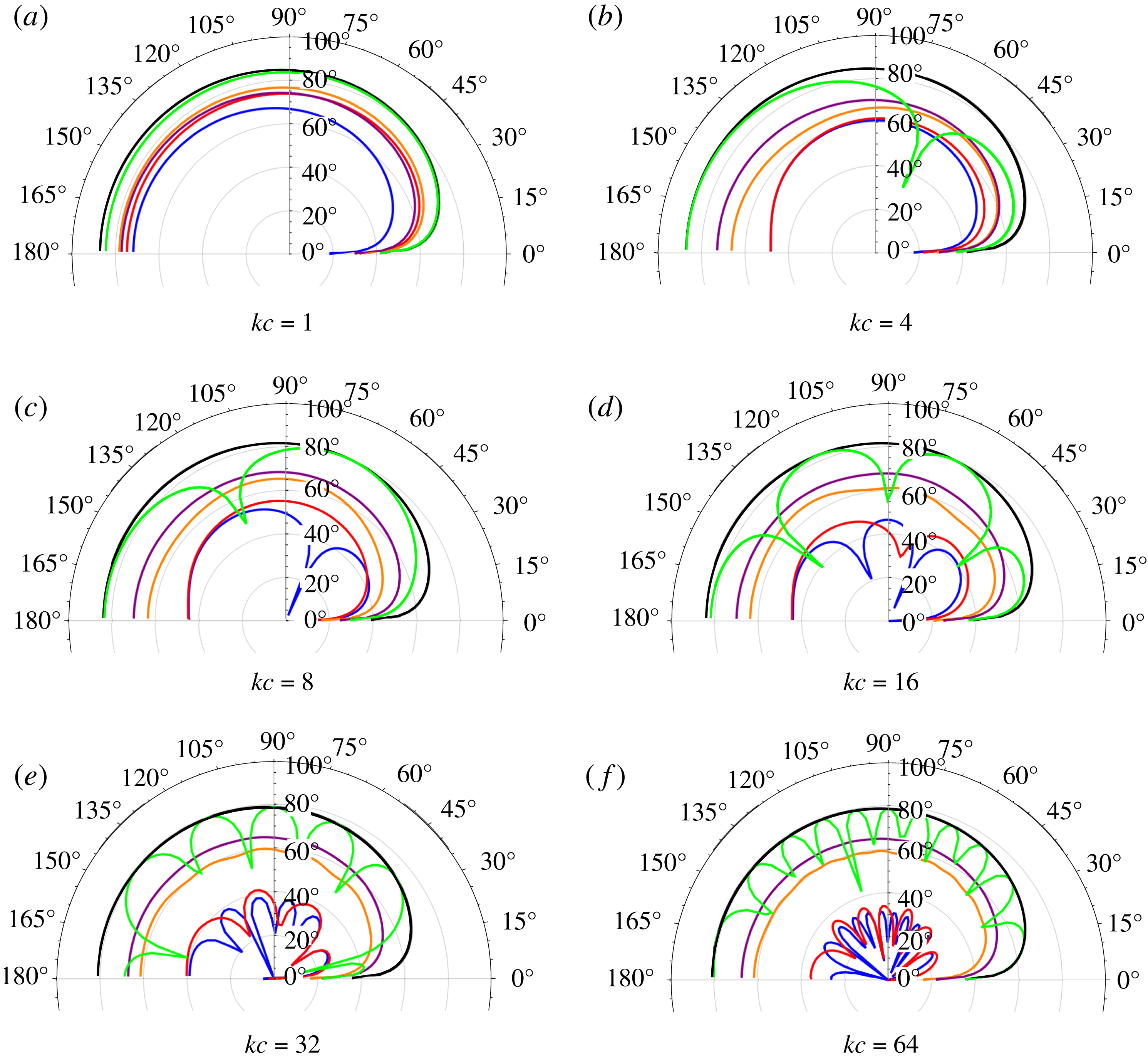
In figure 6 we show the mid-span (
 $z=0.5$
) directivity patterns at
 $r=10$
for a variety of values of
 $kc$
. To enable all values to be easily visible, we add a constant reference value of
 $20\log _{10}10^{6}$
to each SPL. We see the directivities overall follow the same trends as figure 4 despite having variations with observer angle as
 $kc$
increases. The sawtooth (S), v-root (SV) and square wave (SQ) all exhibit strong oscillations with varying observer angle (again illustrating their strong tip and root interference), therefore we must be careful to include a range of observer angles when determining the overall effectiveness of these edges. For example, measuring only at
 $\unicode[STIX]{x1D703}=90^{\circ }$
could overpredict the noise reduction if this coincides with a minimum in the directivity oscillations. These oscillations can also cause different edges to appear optimal at a given
 $kc$
value and given observer angle, when overall they are not: figure 6(d) shows the sawtooth (S) generating more noise at
 $\unicode[STIX]{x1D703}=90^{\circ }$
than the v-root (SV), but further towards the downstream direction,
 $\unicode[STIX]{x1D703}=130^{\circ }$
, the sawtooth generates significantly less noise than the v-root.
Over almost all observer angles there is a reduction of far-field noise, as observed by Sanjose et al. (Reference Sanjose, Meon, Masson and Moreau2014). In the wake direction (
 $\unicode[STIX]{x1D703}=0$
) Sanjose et al. (Reference Sanjose, Meon, Masson and Moreau2014) observe a slight noise increase, which we do not see here. This may be caused by the vortex shedding (more precisely the reduction of vortex shedding) by the serrated edge. As our simple analytical model assumes a vortex sheet for the wake, we cannot assess any effects of altered vortex shedding, and therefore do not recreate this result.
Far-field SPL directivities,
 $20\log _{10}(10^{6}|h(10,\unicode[STIX]{x1D703},0.5)|)$
, for
 $M=0.1$
,
 $k_{3}=0$
. Colours match figure 4: straight, black; S, blue; SV, red; SU, orange; CP, purple; SQ, green.

4.4 Far-field sound spectra
In the previous two sections we have focused on
 $k_{3}=0$
; however, to have a prediction of a realistic level of noise scattered by a trailing edge we must include a range of
 $k_{3}$
values. To do so, we define the far-field power spectral density (PSD) as
 $$\begin{eqnarray}\text{PSD}=10\log _{10}\left(\int _{-\infty }^{\infty }|h(r,\unicode[STIX]{x1D703},z)|^{2}\unicode[STIX]{x1D6F1}(\unicode[STIX]{x1D714},k_{3})\,\text{d}k_{3}\right),\end{eqnarray}$$
where
 $$\begin{eqnarray}\unicode[STIX]{x1D6F1}(\unicode[STIX]{x1D714},k_{3})\sim \frac{(\unicode[STIX]{x1D714}/U_{c})^{2}}{(((\unicode[STIX]{x1D714}/U_{c})^{2}+k_{3})^{2}+L^{2})^{2}}\end{eqnarray}$$
is the leading-order approximation from Howe (Reference Howe1991a
) for the wavenumber spectral density in a turbulent boundary layer proposed by Chase (Reference Chase1987) (and that used by Lyu et al. (Reference Lyu, Azarpeyvand and Sinayoko2016)) under the assumption
 $k_{1}\approx \unicode[STIX]{x1D714}/U_{c}$
. Overall multiplicative constants which are independent of the edge geometry have been removed from this definition for clarity. The parameter
 $L$
is defined as
 $L=\unicode[STIX]{x1D712}/\unicode[STIX]{x1D6FF}_{BL}$
, where
 $\unicode[STIX]{x1D712}\sim 1.33$
is provided by Chase (Reference Chase1987), and
 $\unicode[STIX]{x1D6FF}_{BL}$
is the (non-dimensional) boundary layer thickness. We too use the value
 $\unicode[STIX]{x1D712}=1.33$
in this paper in accordance with previous analytic models (Howe Reference Howe1991a
,Reference Howe
b
; Lyu et al.
Reference Lyu, Azarpeyvand and Sinayoko2016), although note that in different experimental and numerical set-ups this parameter (and indeed the assumption
 $U_{c}\approx 0.7U$
) can vary.
In figure 7 we present the far-field PSD for each of the trailing-edge geometries at
 $\unicode[STIX]{x1D703}=90^{\circ }$
. We see the oscillatory behaviour of the SPL (figure 4) is weakened but still present, and we see once again that sharper serrations (larger values of
 $c$
) generally result in a larger noise reduction at a given frequency for each geometry. What differs in the PSD compared to the SPL, however, is the noise reduction for high frequencies: we see that when including a spectrum of
 $k_{3}$
values, the PSD reduction for any serrated edge versus a straight edge can be decreased at high frequencies. There is therefore additional noise created by the serrated edges by
 $k_{3}\neq 0$
components which is not created by the straight edge, particularly at high frequencies. This can be seen from the modes scattered by the serrated edge, (3.9): for
 $k_{3}\sim 2n\unicode[STIX]{x03C0}$
the
 $n$
th mode will always be cut-on. This mode does not exist for a straight edge, whose only scattered frequency is
 $w_{0}^{2}=(k/\unicode[STIX]{x1D6FD})^{2}-k_{3}^{2}$
. The redistribution of energy from lower cut-on modes to higher cut-off modes discussed for
 $k_{3}=0$
now becomes more complicated as the higher modes that energy is redistributed to for increasing frequency or tip-to-root height (increasing
 $kc$
) become cut-on when including sufficiently large
 $k_{3}$
spectral values.
Far-field PSD, for
 $M=0.1$
,
 $L=1.33/0.5$
. Colours match figure 4: straight, black; S, blue; SV, red; SU, orange; CP, purple; SQ, green.

4.5 Comparison with experimental measurements
In this section we compare the analytically predicted far-field reduction of PSD with previous analytical, numerical and experimental measurements, for a sawtooth (S) trailing edge versus a straight trailing edge.
In the analytic model in this paper the mean flow is always parallel to the serrated edge, and we use a simple wall turbulence model described by the wavenumber spectrum (4.7), as assumed by Howe (Reference Howe1991b
) and Lyu et al. (Reference Lyu, Azarpeyvand and Sinayoko2016). It is known that total aerofoil angle of attack (Gruber Reference Gruber2012) and relative misalignment angle of the serrations to the chord (Leon et al.
Reference Leon, Merino-Martínez, Ragni, Avallone, Scarano, Probsting, Snellen, Simons and Madsen2017) can have a significant effect on the predicted far-field noise (up to
 ${\sim}4$
dB and
 ${\sim}10$
dB respectively for large angles). In Leon et al. (Reference Leon, Merino-Martínez, Ragni, Avallone, Scarano, Probsting, Snellen, Simons and Madsen2017) these effects are attributed to the distorted near-surface mean flow and the formation of streamwise turbulent structures. The simple wavenumber spectrum used analytically would likely be unsuitable for describing the turbulence over a serrated trailing-edge aerofoil at significant angle of attack or with misaligned serrations due to their effect on the turbulent structures. Additionally, the effect of vortex shedding, which will occur particularly prominently for aerofoils with serrations cut into the main body (thus having regions along the trailing edge with blunt sections) is not accounted for in the analytical model, although this will produce a discrepancy of tonal rather than broadband noise.
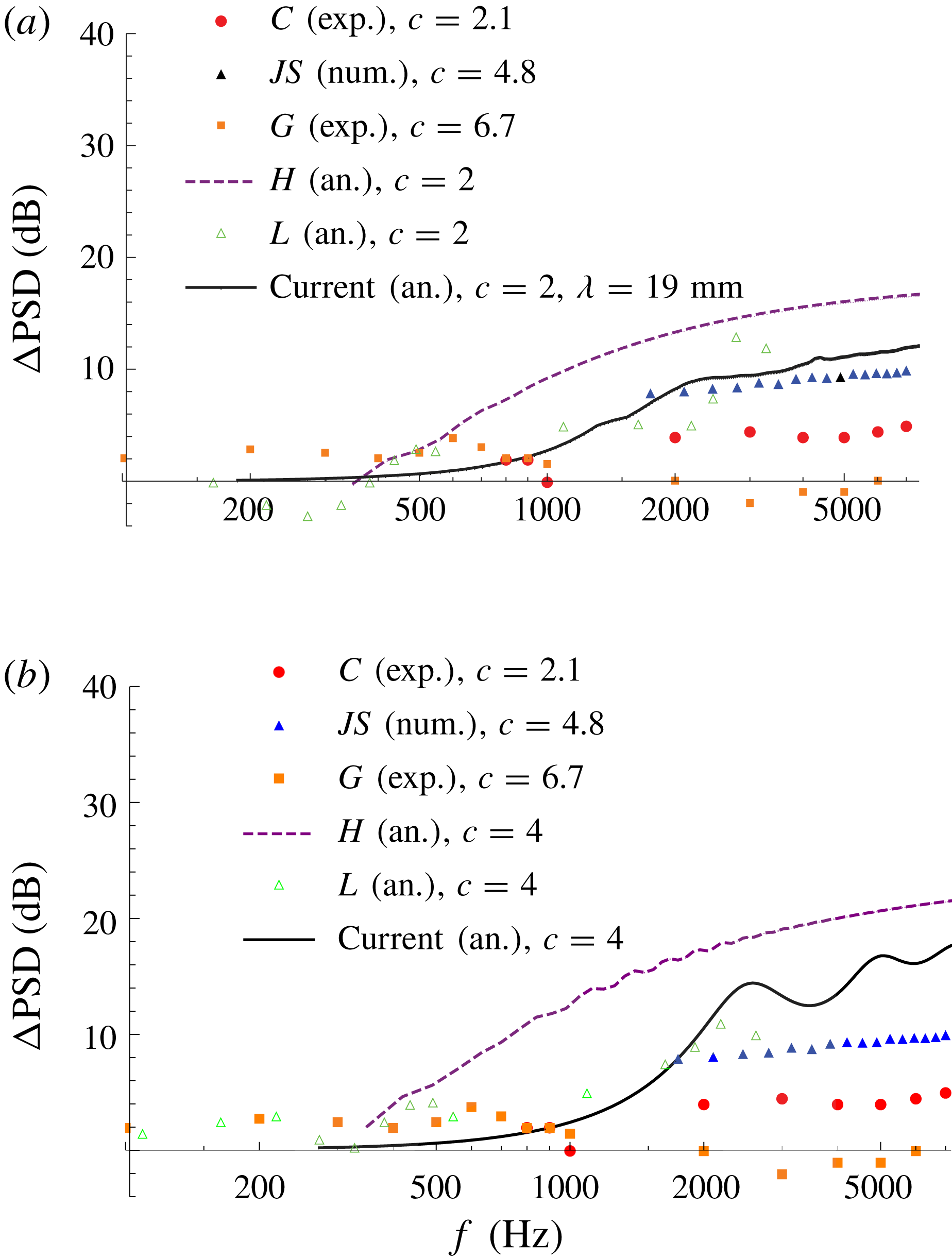
We compare our new analytic solution against a variety of experimental, numerical, and previous analytical models in figure 8. Compared to Howe’s analytical model, the current analytic prediction for noise reduction is reduced, as would be expected given the known overprediction of Howe’s results (Winkler et al.
Reference Winkler, Moreau and Carolus2010; Lyu et al.
Reference Lyu, Azarpeyvand and Sinayoko2016). We see in general good agreement with Lyu’s results (Lyu et al.
Reference Lyu, Azarpeyvand and Sinayoko2016), and mention again, on inclusion of a
 $k_{3}$
wavenumber spectrum, the higher-order modes (which are neglected by Lyu) become important as modes with
 $k_{3}\sim 2n\unicode[STIX]{x03C0}$
,
 $n\in \mathbb{Z}$
, always propagate to the far field.
PSD noise reduction in dB for a serrated edge versus a straight edge as a function of frequency (Hz). Experimental results taken from Chong et al. (Reference Chong, Vathylakis, Joseph and Gurber2013, figure 9) (red dots) for a NACA 0012 aerofoil at
 $4.2^{\circ }$
angle of attack with
 $U_{\infty }=51~\text{m}~\text{s}^{-1}$
. Numerical results (blue triangles) taken from Jones & Sandberg (Reference Jones and Sandberg2012, figure 6) for NACA 0012 aerofoil at
 $5^{\circ }$
angle of attack, with
 $M=0.4$
. Experimental results taken from Gruber (Reference Gruber2012, figure 4.4) (orange squares) for a NACA 65(12)-10 aerofoil at
 $5^{\circ }$
angle of attack, with
 $U_{\infty }=40~\text{m}~\text{s}^{-1}$
. Previous analytical results are from Howe (Reference Howe1991b
, (18)) (purple dashed line, with
 $h/\unicode[STIX]{x1D6FF}=8$
as defined in Howe’s solution) and Lyu et al. (Reference Lyu, Azarpeyvand and Sinayoko2016, figure 6c) (green triangles), both taken directly above the trailing edge at
 $\unicode[STIX]{x1D703}=90^{\circ }$
. Current analytic results (black line) calculated from (4.6) use
 $L=1.33/0.5$
, taken at
 $\unicode[STIX]{x1D703}=90^{\circ }$
. (a) Analytic solutions with
 $c=2$
,
 $M=0.1$
,
 $\unicode[STIX]{x1D706}=19$
mm (as used by Chong et al. (Reference Chong, Vathylakis, Joseph and Gurber2013, figure 9)). (b) Analytic solution with
 $c=4$
,
 $M=0.1$
, and
 $\unicode[STIX]{x1D706}=9$
mm (as used by Gruber (Reference Gruber2012, figure 4.4)).

The poor agreement with the experimental results of Gruber (Reference Gruber2012) is attributed to the high effective angle of attack at the trailing edge (due to both an angle of attack of the flow, and a cambered aerofoil).
The numerical results of Jones & Sandberg (Reference Jones and Sandberg2012), found through direct numerical simulation, show a similar trend to Howe’s predictions, in that there is no drop-off of noise reduction at higher frequencies. This is mirrored in the experimental results of Chong et al. (Reference Chong, Vathylakis, Joseph and Gurber2013), and indeed in our new analytical model to the frequencies investigated in figure 8. As the numerical and experimental results are at a
 ${\sim}5^{\circ }$
angle of attack, we can expect up to
 ${\sim}4$
dB difference in noise reduction (Gruber Reference Gruber2012) versus the flat-plate case investigated analytically at high frequencies, which is seen here.
We also mention that at low frequencies the steepest descent approximation made prior to (3.18) is no longer valid, therefore we expect discrepancies between our current analytic results and all other results for
 $f\lessapprox 400$
Hz.
Overall it is clear from the results present in figure 8 that there is great variation in the prediction of noise reduction for serrated trailing edges, due to a variety of aerofoil and flow parameters. However, overall the new analytic results found in this paper are an improvement over Howe’s predictions and can form a basis for developing more involved analytical models which could take into account angle of attack or geometry. Furthermore, the new solution presented in this paper can account for all propagating modes and does not require an iterative numerical procedure to produce results, which is an improvement over the method presented by Lyu et al. (Reference Lyu, Azarpeyvand and Sinayoko2016).
5 Conclusions
In this paper we have found an analytic solution for the far-field noise generated by the turbulent boundary layer scattering off of a trailing edge which is permitted some periodic spanwise variation in geometry. The analytic solution, obtained via the use of a non-orthogonal coordinate transformation, separation of variables and the Wiener–Hopf technique, leads to a closed-form prediction of the far-field noise. The solution limits to the known straight-edge solution as the serration height is sent to zero, and compares well with the previous semi-analytic results of Lyu et al. (Reference Lyu, Azarpeyvand and Sinayoko2016) for sawtooth serrations both with small and large tip-to-root ratios. With this simple analytic expression for the far-field pressure, we have investigated the effects of different trailing-edge geometries on the overall noise levels, and proposed mechanisms which allow different geometries to reduce the noise levels differently.
There are two key mechanisms of noise reduction. First a destructive interference of tip and root fields, which dominates in the low and mid-frequency ranges, and is most beneficial for the square wave (SQ) geometry. Second, a redistribution of energy from low propagating modes to higher cut-off modes, which dominates in the high frequency range, and is only fully effective for geometries without any flat sections, such as the serration (S) and slitted v-root serration (SV). When considering a spectrum of
 $k_{3}$
values this second feature is impeded: higher modes become cut-on for
 $k_{3}\sim 2n\unicode[STIX]{x03C0}$
, and therefore do still propagate to the far field.
We have seen that very large noise reductions can be seen at specific observer angles in the far field, but due to modulated directivity patterns if one considers the whole range of observer angles the noise reduction is lessened (but still effective). One must therefore be careful if conducting experiments to measure a sufficiently large range of observer angles to avoid overpredicting the noise reduction possible for a given trailing-edge design.
It is known that a trailing-edge spanwise variation can affect the turbulent structures at the trailing edge (Avallone, Probsting & Ragni Reference Avallone, Probsting and Ragni2016), therefore it is unclear if using the simplistic wavenumber spectrum from Chase (Reference Chase1987) is sufficiently realistic to predict true noise reductions from serrated trailing edges. It may be valuable to develop a new wavenumber spectrum that realistically matches the wall pressures measured experimentally at serrated trailing edges. This analytic method would still work with any such appropriate spectrum. It is also known that serrated trailing edges can significantly affect the structure of the turbulent wake (Jones & Sandberg Reference Jones and Sandberg2012; Sanjose et al. Reference Sanjose, Meon, Masson and Moreau2014) and in particular the structure of the shed vortices. Since this analytic model uses a vortex sheet it does not account for any alterations to the wake due to the existence of the serrations.
Whilst we have only considered five test-case geometries in this paper, the method permits any single-valued periodic geometry. This work can therefore be used to predict the optimal version of any trailing-edge design, such as the optimal slit width for a slitted v-root serration. This, of course, should be balanced with minimising the aerodynamic impact of reducing the surface area at the trailing edge, and should be a subject of future research.
Acknowledgement
The work in this paper was supported by EPSRC Early Career Fellowship EP/P015980/1.