1. Introduction
This paper is about the impact of immigration on the US macroeconomy. Immigration has become an important issue in the USA because of the increase in immigration since the 1960s. Research on the macroeconomic effects of immigration is scarce. I fill this gap by using structural vector autoregressions (SVARs) to address (i) the macroeconomic effects of immigration on the US labor market, (ii) whether or not the short- and long-run effects of immigration differ, (iii) the impact of aggregate productivity, labor demand, transitory consumption, and news shocks on immigration, and (iv) whether or not these effects change over time.
Several papers use SVARs to study the impact of immigration on the aggregate economy; see Boubtane et al. (Reference Boubtane, Coulibaly and Rault2013), Dalbis et al. (Reference Dalbis, Boubtane and Coulibaly2016), Kiguchi and Mountford (Reference Kiguchi and Mountford2019), and Furlanetto and Robstad (Reference Furlanetto and Robstad2019). However, no consensus has been reached on the identification and the macroeconomic effect of a shock to immigration. I contribute to this literature by estimating SVARs using a novel approach to identification and accounting for several changes in US immigration policy beginning with the 1965 Immigration and Nationality Act.
Identification of the SVARs in this study builds on GalÍ (Reference GalÍ1999). GalÍ’s approach is useful because he identifies a total factor productivity (TFP) shock by assuming it is the only shock that has a permanent effect on average labor productivity (ALP) in the long run. The second variable in the SVARs is hours worked. GalÍ identifies its forecast innovation as a demand shock. Starting from this SVAR, I introduce immigration to study its impact on the macroeconomy. The identification of a supply shock to immigration combines short- and long-run restrictions. One restriction is immigration does not respond to other macroeconomic shocks on impact. This reflects the fact that the decision to immigrate responds to changes in economic conditions only with a lag (Borjas (Reference Borjas2006)).
Along with the short-run restrictions, two alternative restrictions are considered for the long-run impact of the immigration supply shock on ALP. In the first identification, ALP is assumed to be long-run neutral with respect to an immigration supply shock. The alternative assumes ALP responds to an immigration supply shock in the long run. The motivation for these identifying restrictions is the lack of consensus on the long-run relationship between immigration and productivity, as documented in Feyrer (Reference Feyrer2007) and Ortega and Peri (Reference Ortega and Peri2013), among others.
This does not completely identify the immigration supply shock. The reason is the decision to migrate is forward-looking with respect to news about productivity and expected changes in lifetime earnings (i.e., permanent income). To disentangle the forward-looking aspect of immigration, I first identify a news shock by including the Treasury term spread to apply short- and long-run restrictions as in Beaudry et al. (Reference Beaudry, Feve, Guay and Portier2019) and Forni et al. (Reference Forni, Gambetti and Sala2019). Further, adding consumption to the SVARs identifies a transitory consumption shock. This is to account for the expectations immigrants have about permanent income.
Another important component pertaining to the macroeconomic dynamics of immigration is policy. There have been several changes to US immigration policy since the 1960s. These policy changes have the potential to induce structural change in immigration shocks that are revealed through drifting persistence and/or volatility. Therefore, I estimate a baseline SVAR with time-varying parameters (TVPs) and stochastic volatility (SV). Addressing structural change in data is important in reaching reliable estimates of SVARs, as stressed by Sims and Zha (Reference Sims and Zha2006) and Nason and Tallman (Reference Nason and Tallman2015). I explore the data with respect to TVP, SV, and different identification schemes in a Bayesian model selection exercise.
To my knowledge, this paper is the first to identify an immigration supply shock using short- and long-run restrictions and to allow time variation in the SVAR. For example, Kiguchi and Mountford (Reference Kiguchi and Mountford2019) use a sign-restricted SVAR to show output per capita falls in the short run following an immigration shock. With Norwegian data, Furlanetto and Robstad (Reference Furlanetto and Robstad2019) assume immigration is a substitute for domestic labor supply in a SVAR. They conclude that an immigration shock has a negative effect on labor productivity. Boubtane et al. (Reference Boubtane, Coulibaly and Rault2013) and Dalbis et al. (Reference Dalbis, Boubtane and Coulibaly2016) identify an immigration shock in a Choleski recursive ordering with GDP per capita and labor input for OECD countries. They find that GDP per capita and other aggregate variables rise in response to an immigration shock. Compared to these studies using fixed-coefficient SVARs, this paper contributes to the immigration literature in documenting substantial time variation in the impact immigration has on the US macroeconomy over the business cycle horizons and in the long run. This paper is also the first in providing macroeconomic evidence of time variation associated with episodes of changes in US immigration policy since the 1960s.
Estimates of the SVARs yield several conclusions about the impact of immigration on the US economy. First, the data strongly favor an identification scheme that allows ALP to respond to the immigration supply shock in the long run. The impulse response functions (IRFs) of the data-favored SVAR indicate ALP and hours worked increase at the business cycle horizons to an immigration supply shock. The medium- to long-run responses of ALP and consumption to an immigration supply shock diminish over the sample, which coincide with the 1986 and 1990 immigration policy changes. Immigration responds positively to an increase in productivity and positive news about future productivity, but these IRFs display substantial time variation that also depend on changes to immigration policy.
The major source of immigration fluctuation in the USA is its own supply shock. Nevertheless, TFP and news shocks matter for driving short- and long-run immigration. On the other hand, the immigration supply shock plays an important role in the forecast error variance decompositions (FEVDs) of consumption and the term spread.
These findings indicate that (i) immigration has had a positive impact on the US economy at the business cycle horizons and in the long run, (ii) the immigration supply shock is important to the US macroeconomy, and (iii) the macroeconomic effects of immigration are dependent on the structure of US immigration policy. Peaks in the SV of the immigration supply shock match episodes of changes in US immigration policy. For instance, the SV peaks at the time the Immigration Act of 1990 is passed by Congress. Therefore, disentangling the impact of the immigration supply shock from its SV is important for evaluating the role immigration plays in the US macroeconomy.
The remainder of this paper is organized as follows: Section 2 discusses historical changes in immigration policy and the data. Section 3 presents identification and estimation of the SVARs. Section 4 provides results. Section 5 concludes.
2. US immigration policy and data
This section gives a brief review of changes to US immigration policy. This is followed by a discussion on the data source and interpolation.
2.1. Background on recent changes to immigration policy
Eight major immigration policy changes are relevant to this paper. Among these are changes in the quota of various categories of immigration, level of border patrol enforcement, and amnesty for irregular immigrants. Footnote 1 Changes to immigration policy are important in identifying the aggregate effects of immigration on the US economy. These changes affected the flow of immigration to the USA in several ways.
The Immigration and Nationality Act of 1965 (INA, also known as the Hart-Celler Act) first permitted non-Caucasian immigration, which had been prohibited since 1924. The Act had important long-run implications on the demographic composition of immigration, number of new immigrants, and migration decision. The enactment of the Refugee Act of 1980 and the Immigration Reform and Control Act of 1986 (IRCA) began an era of nonrestrictive immigration policies by creating new categories of permanent immigration and a nationwide amnesty of irregular immigration. Coupled with the American Homecoming and Immigration Act of 1990 (IMMACT), which increased immigration quota, these changes in immigration policy raised quarterly immigration influx by almost threefold, peaking at 1990Q1. Between the mid-1990s and the 2001 dot-com bubble, quotas for employment-based visa (and effectively the number of employment-based permanent residency applications) were raised three times in 1990, 1998, and 2000 up to 195,000, before it decreased to its pre-1990 level of 65,000 in 2004 through the H-1B Reform Act. The re-adjustment of quota generated kinks in at least the employment-based category of permanent immigration. Changes in these policies could also induce structural breaks in immigration. Given the history of US immigration policy during the sample, it is important to study the macroeconomic dynamics of immigration using an empirical model that can account for structural change in the US economy tied to changes in immigration policy.
2.2 Data
I use time series on the flow of new permanent residency as the measurement of immigration. I assume this measure of immigration proxies for the number of new immigrants eligible to work in the US labor market. Footnote 2 The source is Yearbook of Immigration Statistics published by the DHS. This series contains annual flow of foreign-born civilian admittance to the USA by category but excludes temporary immigration admittance (nonimmigrant visa holders) such as foreign students or visitors. The sample covers 1953–2017. Footnote 3
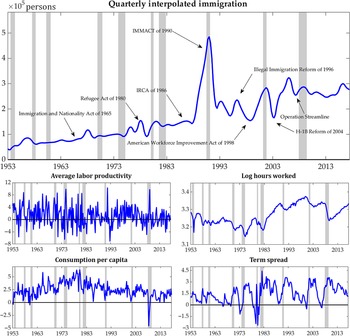
A problem with the DHS immigration data is its low frequency at an annual rate. I interpolate the official annual series to quarterly from 1953Q1 to 2017Q4 using a regression-based approach developed by Silva and Cardoso (Reference Silva and Cardoso2001). Footnote 4 The top panel of Figure 1 plots the interpolated quarterly immigration. Eight major immigration policy dates are labeled with arrows. Immigration begins to resemble a unit root process after the enactment of the 1965 INA. Until 1990, immigration displays a positive trend and the fluctuations around trend are small. There is a large peak in immigration from 1988 to 1991, which coincides with the enactment of the 1986 IRCA and the 1990 IMMACT. This peak subsides by 1993. Immigration reverts to the pre-1990 trend after the peak but exhibits greater volatility around the trend.
Data.
Notes: The sample size ranges from 1953Q1 to 2017Q4. Immigration policy reform dates are labeled with arrows. Gray shaded areas are NBER recession trough dates. X-axis: sample date; y-axis:
 $10^5$
persons (immigration), percentage points (ALP, consumption, term spread), log points (hours worked).
Source: Yearbook of Immigration, Bureau of Labor Statistics, Cociuba et al. (Reference Cociuba, Prescott and Ueberfeldt2018), and FRED.

I test for unit roots in the growth rate and log levels of immigration. Augmented Dickey–Fuller test rejects the existence of unit root at 1% when the series is in growth rate but not in log levels. As a result, the interpolated quarterly immigration series is treated as observationally equivalent to an I(1) series. However, I note that structural breaks can be responsible for creating random walk like behavior in immigration.
Figure 1 also contains four other macroeconomic indicators on which the SVARs are estimated. ALP is utilization-adjusted following Basu et al. (Reference Basu, Fernald and Kimball2006). Hours worked is log weekly hours per capita. Consumption is a Fisher ideal index of constant dollar services and nondurable goods per capita consumption expenditures. Treasury term spread is the difference between yield on 10-year constant maturity Treasury and yield on 90-day Treasury.
3. TVP-SV-SVARs
This section presents the TVP-SV-SVARs and the identification schemes. I focus on the assumptions and restrictions that identify the immigration supply shock. Estimation of SVARs relies on a Bayesian Markov Chain Monte Carlo (MCMC) algorithm. A Bayesian model selection exercise compares the log-marginal data densities of several models.
3.1 The TVP-SV-SVAR
The data vector
 $z_t = [\Delta{\log}(x_t),\, {\log}(n_t),\,\Delta{\log}(I_t), \,\Delta{\log}(c_t), \, s_t]$
collects ALP growth (
 $\Delta{\log}(x_t)$
), log weekly hours (
 ${\log}(n_t)$
), immigration growth (
 $\Delta{\log}(I_t)$
), consumption growth (
 $\Delta{\log}(c_t)$
), and the term spread (
 $s_t$
).
Footnote 5
I estimate
 \begin{equation*}z_t = b_{t} + \sum_{l=1}^p{B}_{l,t}z_{t-l} + A_{0,t}^{-1}\Sigma_t^{\frac{1}{2}}\epsilon_t, \quad \epsilon_t \sim N(0, I),\end{equation*}
where
 $b_{t}$
denotes the
 $5\times1$
row vector of time-varying constants,
 ${B}_{l,t}$
are
 $5\times5$
matrices of the reduced-form TVPs for lags
 $l=1,...,p$
and
 $t=1, ..., T$
. The impact matrix
 $A_{0,t}$
has ones on the diagonal and can be non-recursive for the off-diagonal elements. The
 $5\times5$
diagonal matrix
 $\Sigma_t^{\frac{1}{2}} = diag\{\sigma_{k,t}\}$
collects the square roots of the SVs of the structural shocks
 $\epsilon_t$
at t along the diagonal with zeroes everywhere else. The concentrated form of the SVAR is
 \begin{equation}A_{0,t}(z_t - X_t'\mathbb{B}_t) = \Sigma_t^{\frac{1}{2}}\epsilon_t,\end{equation}
where
 $X_t' = I_{n}\otimes[z_{t-1}'...\,z_{t-p}'\,1]$
and
 $\mathbb{B}_t = [vec({B}_{1,t})'...\,vec({B}_{p,t})'\,b_t]'$
. The off-diagonal entries in
 $A_{0,t}$
represent the contemporaneous restrictions. I denote
 $a_{jk,t}$
the free elements in
 $A_{0,t}$
.
As is customary in the TVP-VAR literature, parameter blocks
 $(\mathbb{B}_t, \, A_{0,t}, \, \sigma_{k,t})$
are treated as latent variables that evolve as driftless random walks and geometric random walks:
 \begin{equation}p(\mathbb{B}_t|\mathbb{B}_{t-1},Q) = I(\mathbb{B}_t)f(\mathbb{B}_t|\mathbb{B}_{t-1},Q),\end{equation}
 \begin{equation}a_{jk,t} = a_{jk,t-1} + \zeta_{t},\end{equation}
 \begin{equation}log(\sigma_{k,t}) = log(\sigma_{k,t-1}) + \tau_{k,t},\end{equation}
where
 $I(\mathbb{B}_t)$
is an indicator function that rejects unstable draws of
 $\mathbb{B}_t$
, the law of motion
 $f(\mathbb{B}_t|\mathbb{B}_{t-1},Q)$
is given by
 $\mathbb{B}_t = \mathbb{B}_{t-1} + \eta_t$
. Let
 $\tau_t = [\tau_{1,t},...,\tau_{5,t}]$
, then
 $[\eta_t, \zeta_t, \tau_t]$
are mean zero,
 $i.i.d.$
disturbances with variance–covariance matrices [Q, S, W].
Putting the blocks of latent variables together yields
 \begin{equation}\mathcal{V} = Var\left(\begin{bmatrix} \epsilon_t \\ \eta_t \\ \zeta_t \\ \tau_t \\ \end{bmatrix}\right) = \begin{bmatrix} I_5 & 0 & 0 &0\\ 0 & Q & 0 &0\\ 0 & 0 & S &0\\ 0 & 0 & 0 &W\\ \end{bmatrix},\end{equation}
where Q, S, and W are full rank. Note that this setup accommodates SVARs lacking TVPs and/or SV. The estimation of a static-coefficient SVAR requires setting
 $Q = S = W =0$
. A TVP-SVAR with no SV sets
 $W =0$
. A static-coefficient SVAR with SV sets
 $Q = S = 0$
.
3.2. Identification
This section outlines the strategies I use to identify the SVARs. I employ a novel set of short- and long-run restrictions to identify a supply shock to immigration. I label the immigration shock a supply shock following Borjas (Reference Borjas2003). The definition of immigration in this paper is similar to Borjas’ notion of influx of immigrants to the USA that he refers to as immigration supply. This is also to clarify that I am not identifying an immigration policy shock.
The complication in identifying the immigration supply shock stems from the endogeneity of immigration. Forward-looking immigrants self-select into countries and labor markets in which they anticipate their job market prospects are best (Friedberg (Reference Friedberg2001), Borjas (Reference Borjas2003)). To identify an immigration supply shock in the macroeconomy, the permanent income hypothesis and news about future TFP shocks are used to tackle the forward-looking aspect of immigration.
The five identified shocks are TFP, labor demand, immigration, transitory consumption, and news about future TFP. Footnote 6 This section concludes with a comparison of four identification schemes and specifications on TVP and/or SV. A Bayesian model selection exercise explores the preference the data have over the competing models.
3.2.1 Short-run restrictions
Following standard practice in the immigration literature (e.g., Pischke and Velling (Reference Pischke and Velling1997), Card (Reference Card2007), Dalbis et al. (Reference Dalbis, Boubtane and Coulibaly2016)), the first identifying assumption is migration decisions are made prior to the entry date. Partridge and Rickman (Reference Partridge and Rickman2009) document the delayed migration response to changes in economic conditions. Therefore, the response of immigration to macroeconomic incentives lags the date an immigrant enters the labor market. Imposing this restriction on
 $A_{0,t}$
yields the first set of short-run identifying restrictions:
 \begin{equation*}\text{SR1}: \quad\quad a_{31,t} = a_{32,t} = a_{34,t} = a_{35,t} = 0.\end{equation*}
These short-run identifying restrictions force immigration to react only to its own shock at impact.
The news shock literature (Forni et al. (Reference Forni, Gambetti and Luca2014), Beaudry et al. (Reference Beaudry, Feve, Guay and Portier2019), among others) identify ALP to only respond to its own shock on impact. I use this as the second set of short-run restrictions which consists of
 \begin{equation*}\text{SR2}: \quad\quad a_{12,t} = a_{13,t} = a_{14,t} = a_{15,t} = 0.\end{equation*}
Note the immigration supply shock affects ALP only with a lag. Stated differently, I assume immigration faces labor market rigidity of at least one quarter.
A neoclassical model of the labor market predicts immigration causes labor productivity to fall and hours worked to rise; see Card (Reference Card2001) and Borjas (Reference Borjas2006). Nonetheless, the microeconomics literature on immigration often reports conflicting empirical evidence about the impact of immigration on labor market outcomes, according to Kerr and Kerr (Reference Kerr and Kerr2011). Given no clear advice, I leave the impact response of hours worked to an immigration supply shock unrestricted.
Finally, an inflow of immigration affects consumption. There are studies documenting the effect immigration has on the receiving economy through a change in consumption expenditure. For instance, Coppel et al. (Reference Coppel, Dumont and Visco2001) and Hong and McLaren (Reference Hong and McLaren2016) find immigration increases consumption, because immigration enlarges an economy through an immediate increase in the number of households. However, since there is little evidence on whether this effect occurs at impact or with a lag, I consider two alternatives. The first option imposes
 \begin{equation*}\text{SR3}: \quad\quad a_{43,t} = 0.\end{equation*}
Under SR3, consumption responds to the immigration supply shock with a lag. The alternative assumes that consumption reacts to the immigration supply shock at impact, which implies
 $a_{43,t}$
is estimated.
To sum up, I consider two short-run identifications:
 \begin{equation}A_{0,t}^I = \begin{bmatrix} 1 & 0 & 0 & 0 & 0\\ a_{21,t} & 1 & a_{23,t} & a_{24,t} & a_{25,t}\\ 0 & 0 & 1 & 0 & 0\\ a_{41,t} & a_{42,t} & a_{43,t} & 1 & a_{45,t}\\ a_{51,t} & a_{52,t} & a_{53,t} & a_{54,t} & 1\\ \end{bmatrix} \,\, \text{and}\,\, A_{0,t}^{II} = \begin{bmatrix} 1 & 0 & 0 & 0 & 0\\ a_{21,t} & 1 & a_{23,t} & a_{24,t} & a_{25,t}\\ 0 & 0 & 1 & 0 & 0\\ a_{41,t} & a_{42,t} & 0 & 1 & a_{45,t}\\ a_{51,t} & a_{52,t} & a_{53,t} & a_{54,t} & 1\\\end{bmatrix}.\end{equation}
The impact matrix
 $A_{0,t}^I$
only imposes SR1 and SR2, while
 $A_{0,t}^{II}$
imposes SR1, SR2, and SR3. For both alternatives, consumption is allowed to respond to the TFP shock on impact following the permanent income hypothesis. A TFP shock permanently raises the household income and therefore consumption expenditure. Because of the willingness to smooth consumption over time, the agents take advantage of a higher income by increasing consumption on impact.
3.2.2 Long-run restrictions
A long-run identification is imposed by restricting the elements of the cumulative response matrix,
 $D_t$
. First, compute the cumulative impact matrix:
 \begin{equation}D_t = J(I_{5} - \mathbb{B}_t)^{-1}J'A_{0,t}^{-1}\Sigma_t^{\frac{1}{2}},\end{equation}
where
 $J = [I_5 \dots 0_5]$
is a selection matrix. Denote
 $d_{jk,t}$
the elements in
 $D_t$
, setting
 $d_{jk,t} = 0$
imposes long-run neutrality of variable j to shock k.
Let the restricted long-run cumulative matrix be
 $\tilde{D}_t$
. Solve for the restricted structural intercepts and slope parameters matrix
 $\tilde{\mathbb{B}}_t$
by inverting equation (7). This step is important because the reduced-form parameters in
 $\mathbb{B}_t$
are no longer consistent with the restricted long-run matrix. Imposing long-run restrictions induces nonlinearities to the reduced-form VAR parameter space because of the inversion of the equation. Therefore, I also check the eigenvalues of
 $\tilde{\mathbb{B}}_t$
to ensure stationarity of the SVAR. The implementation of long-run restrictions to (7) requires additional sampling steps that I outline in the following section.
One incentive of immigration is an increase in expected lifetime earnings. For example, Coppel et al. (Reference Coppel, Dumont and Visco2001) and Damette and Fromentin (Reference Damette and Fromentin2013) argue the decision to migrate depends on the economic prosperity of the host country. I assume the anticipated long-run performance of the US economy matters for the immigration decision. Hence, the long-run restrictions rest on the permanent income potential immigrants expect when making the decision to move. Consumption captures these changes in expected lifetime earnings of immigrants. Since immigration is observationally equivalent to an I(1) series, I assume the level of immigration is independent of the transitory labor demand and transitory consumption shocks in the long run. These assumptions are reflected in the first collection of long-run restrictions:
 \begin{equation*}\text{LR1}: \quad\quad d_{32,t} = d_{34,t} = 0.\end{equation*}
The cumulative impact of a TFP shock on immigration,
 $d_{31,t}$
, is left unrestricted. As a result, estimates of
 $d_{31,t}$
measure the incentive to immigrate at the aggregate level.
Another important factor that shapes migration decision is news about TFP. The news shock represents the expectations agents hold about TFP in the future. I identify a news shock to capture the forward-looking nature of migration decision. Following the recent news literature, the identifying restrictions of the news shock include (i) SR2 and (ii) ALP responds to the news shock in the long run. Footnote 7
Immigration may be important to ALP in the long run, but micro-level data show conflicting evidence about the long-run effect of immigration on ALP. Firm-level data show immigration could raise long-run productivity through complementing domestic labor force, technological transfers, or innovation engagement; see Feyrer (Reference Feyrer2007) and Hunt and Gauthier-Loiselle (Reference Hunt and Gauthier-Loiselle2010). On the other hand, Ortega and Peri (Reference Ortega and Peri2013) and Paserman (Reference Paserman2013) find no effect on long-run productivity that is produced by immigration. I consider both alternatives in restricting the long-run response of ALP to an immigration supply shock. Further, I restrict ALP to not respond to labor demand shocks in the long run following GalÍ (Reference GalÍ1999). This identifying restriction assumes transitory demand shocks do not have permanent effects on I(1) variables:
 \begin{equation*}\text{LR2}: \quad\quad d_{12,t} = d_{14,t} = 0,\end{equation*}
and
 \begin{equation*}\text{LR3}: \quad\quad d_{13,t} = 0.\end{equation*}
The former set of restrictions imposes LR3. The immigration supply shock has no long-run impact on ALP. The alternative is to allow immigration supply shock to have long-run effects on ALP. This alternative leaves
 $d_{13,t}$
unrestricted.
Next, consumption is assumed to only respond to TFP, immigration supply, and news shocks in the long run. These responses are embodied in the restrictions:
 \begin{equation*}\text{LR4}: \quad\quad d_{42,t} = d_{44,t} = 0.\end{equation*}
Transitory shocks in labor demand and consumption do not permanently alter consumption. In other words, only I(1) shocks that permanently alter the expected lifetime earnings have a long-run impact on consumption.
In summary, I consider two alternative long-run identification schemes, which are labeled
 $\tilde{D}_t^I$
and
 $\tilde{D}_t^{II}$
,
 \begin{equation}\tilde{D}_t^I = \begin{bmatrix} d_{11,t} & 0 & 0 & 0 &d_{15,t}\\ d_{21,t} & d_{22,t} & d_{23,t} & d_{24,t} & d_{25,t}\\ d_{31,t} & 0 & d_{33,t} & 0 & d_{35,t}\\ d_{41,t} & 0 & d_{43,t} & 0 & d_{45,t}\\ d_{51,t} & d_{52,t} & d_{53,t} & d_{53,t} & d_{55,t}\\ \end{bmatrix}\,\, \text{and}\,\, \tilde{D}_t^{II} = \begin{bmatrix} d_{11,t} & 0 & d_{13,t} & 0 &d_{15,t}\\ d_{21,t} & d_{22,t} & d_{23,t} & d_{24,t} & d_{25,t}\\ d_{31,t} & 0 & d_{33,t} & 0 & d_{35,t}\\ d_{41,t} & 0 & d_{43,t} & 0 & d_{45,t}\\ d_{51,t} & d_{52,t} & d_{53,t} & d_{53,t} & d_{55,t}\\ \end{bmatrix}.\end{equation}
The two long-run identification schemes differ in imposing LR3 on ALP. In
 $\tilde{D}_t^{I}$
, ALP is long-run neutral to an immigration supply shock. In
 $\tilde{D}_t^{II}$
, ALP responds to an immigration supply shock in the long run.
3.2.3 Competing models
Given the short- and long-run identifying restrictions, I list all SVAR specifications using different combinations of these restrictions in Table 1. The two short-run restrictions (
 $A_{0,t}^{I}$
and
 $A_{0,t}^{II}$
) and the two long-run restrictions (
 $\tilde{D}_t^{I}$
and
 $\tilde{D}_t^{II}$
) give four possible identification schemes. Models 1–4 estimate TVP-SV-SVARs with each identification.
Footnote 8
List of models

Notes: TVP denotes time-varying parameters; SV is stochastic volatility; FP denotes fixed-parameter.
I also examine the importance of time variation in the SVAR parameters and in the SVs of the structural errors. I estimate SVARs with four different identifications by turning the TVPs and SVs on and off. Models 5–8 estimate TVP-SVARs with constant SV. Models 9–12 have constant intercepts and slope parameters with SV. Models 13–16 estimate fixed-parameter SVARs. This yields a total of 16 models to be compared in the Bayesian model selection exercise.
3.3 Bayesian estimation
The TVP-SV-SVAR is estimated in state-space form with (1) as the system of observation equations and (2)–(4) as the state equations using a Bayesian MCMC sampler. The goal is to obtain the posterior distribution of the states
 $\mathbb{B}$
,
 $\Sigma$
, and
 $A_0$
using a Metropolis-within-Gibbs sampler developed by Canova and Perez-Forero (Reference Canova and Perez-Forero2015). The SVs are sampled with the 10-component mixture normal routine via a tracking indicator variable (s) À la Omori et al. (Reference Omori, Chib, Shephard and Nakajima2007). A sketch of the sampling steps follows.
Footnote 9
Step 1 Set initial values
 $(\mathbb{B}^T_0, A^T_{0,0}, \Sigma^T_0, s^T_0, \mathcal{V}_0)$
and set
 $i=1$
,
Step 2 Draw the reduced-form intercept and slope parameters
 $\mathbb{B}^T_i$
from
 $p(\mathbb{B}^T_i | z^T, s^T_{i-1}, \Sigma^T_{i-1}, \mathcal{V}_{i-1}) {\cdot} I_B(\mathbb{B}^T_i)$
using the Carter–Kohn algorithm, where
 $I_B(\mathbb{B}^T_i)$
truncates the posterior distribution to ensure the stability of the companion form. Impose long-run identifications for each draw of
 $\mathbb{B}^T_i$
to obtain the structural slope parameters
 $\mathbb{\tilde{B}}^T_i$
,
Step 3 Draw
 $A^T_{0,i}$
from
 $p(A^T_{0,i} | z^T, \mathbb{\tilde{B}}^T_i, s^T_{i-1}, \Sigma^T_{i-1}, \mathcal{V}_{i-1})$
,
Step 4 Draw
 $\Sigma^T_i$
through auxiliary variables
 $s^T_i$
,
Step 5 Draw hyperparameters
 $\mathcal{V}_i$
given
 $(\mathbb{\tilde{B}}^T_i, A^T_{0,i}, \Sigma^T_i, z^T)$
,
Step 6 Repeat step 2 through 4 M times. The last N (
 $<M$
) draws are engaged to construct the posterior of the SVARs.
I set M = 400,000. The burn-in uses the first 200,000 draws. I apply a thinning factor of 50 to the remaining N = 200,000 iterations to reduce the autocorrelation across draws. The baseline TVP-SV-SVAR model produces acceptance rates of the Metropolis step and the rate of stationary draws in the Gibbs step of 24.4% and 32.1%.
4 Results
This section presents estimates of the TVP-SV-SVARs. The SVARs are estimated on a sample from 1963Q1 to 2017Q4. Footnote 10 I discuss results of using Bayesian model selection methods to find which TVP-SV-SVAR the data favors. This is followed by a review of the TVPs and SVs of the SVAR receiving the most support from the data and a discussion on the impact of immigration policy changes on estimates of the TVP-SV-SVARs. This SVAR also produces IRFs and FEVDs. Results of IRFs and FEVDs are displayed toward the end of this section.
4.1 Bayesian model selection results
I report log-marginal data density (LMDD) and Bayes factor (in parentheses, with respect to Model 1) of all the estimated models in Table 2. The LMDDs and Bayes factors of all 16 models are computed using the harmonic mean method by Geweke (Reference Geweke1999).
Results of Bayesian model selection, 1963Q1–2017Q4

Notes: Each entry reports log-marginal data density. Bayes factors (in parentheses) are calculated with respect to Model 1. Log-likelihoods are computed following Geweke (Reference Geweke1999).
 $A_{0,t}^{I}$
imposes SR1 and SR2.
 $A_{0,t}^{II}$
imposes SR1, SR2 and SR3.
 $\tilde{D}_t^{I}$
imposes LR1, LR2, LR3, and LR4.
 $\tilde{D}_t^{II}$
imposes LR1, LR2, and LR4. TVP denotes time-varying parameters; SV is stochastic volatility; FP denotes fixed-parameter. The boldface explain Model 1 is the winner.
First, data strongly favor TVP-SV-SVARs (e.g., Models 1–4) compared to the static-coefficient SVARs (Models 13–16) with all Bayes factors
 $>$
1
 $e^{50}$
. According to Jeffrey’s criterion, a Bayes factor of
 $>$
150 represents decisive model selection preference. Adding TVP or SV improves posterior LMDDs. Comparing the TVP-SVARs and SV-SVARs, the addition of TVP is more important than SV. Nonetheless, the SVARs with both TVPs and SVs better fit the data as we shall see in the following section.
The highest LMDD of
 $-271.73$
is achieved by Model 1. Recall Model 1 imposes short-run neutrality of immigration with respect to all macroeconomic shocks (SR1 and SR2) and leaves the impact response of consumption to the immigration supply shock unrestricted. Model 1 also imposes LR1, LR2, and LR4 but does not restrict the long-run response of ALP to the immigration supply shock.
Given the Bayesian model selection results, the rest of the paper focuses on estimates produced by Model 1.
4.2 SV and TVPs
Time variation in the structural parameters of immigration offers insights about the transmission mechanism of the immigration supply shock. This section presents the SVs of all structural shocks and the time-varying impact parameters that are associated with immigration.
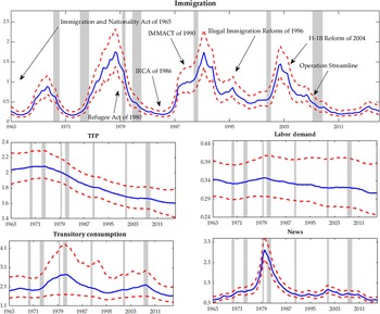
The SV of the immigration supply shock is important for estimating the impact of immigration on the US economy. The first panel of Figure 2 plots the SV of the immigration supply shock with 16–84% posterior tunnels. The shaded areas are NBER recession dates. The arrows point to dates of the immigration policy changes. The SV of the immigration supply shock displays qualitatively and quantitatively meaningful fluctuations over the sample. These fluctuations often occur around changes of immigration policy. For instance, the Refugee Act of 1980 and the H-1B Reform Act of 2004 correspond to two peaks in the SV. However, the INA of 1965, the IRCA of 1986, and IMMACT of 1990 lead their respective peaks in the SV by 2 years. Further, peaks in SV lag the business cycle after 1990 and vice versa prior to 1990. These results indicate that changes in immigration policy alter the SV of the immigration supply shock, but the effect of each episode differs.
Posterior estimates of SVs, estimated with Model 1, 1963Q1–2017Q4.
Notes: The plots contain median posterior estimates of SVs as solid (blue) lines. 16–84 percentile uncertainty bands appear as dotted (red) lines. Immigration policy reform dates are labeled with arrows. The sample period is 1963Q1–2017Q4. X-axis: sample date; y-axis: magnitude of estimate. Gray shades are NBER recession trough dates.

The lower panels of Figure 2 display the SVs of the TFP, labor demand, transitory consumption, and news shocks. There is a prominent downward drift in the SV of TFP starting the productivity slowdown of the 1970s and throughout the Great Moderation. The SV of the news shock also displays large movements around the NBER recession trough dates during the 1980–1982 recessions and around the dot-com bubble of 2001. Therefore, these policy- and business-cycle-dependent changes in the standard deviation of shocks point to the importance of accounting for time variation in the SVs on the macroeconomic dynamics of immigration.
The posterior median values of the impact coefficients associated with immigration (
 $a_{23,t}$
and
 $a_{43,t}$
) are small and oscillate around zero.
Footnote 11
These coefficients are the estimated structural impact coefficients from the short-run restriction matrix
 $A_{0,t}$
. The former controls the contemporaneous effect of immigration on hours worked, and the latter represents that of consumption. In spite of a noticeable degree of time variation, there is no consistent pattern with respect to either the NBER- dated recessions or immigration policy dates. As I shall discuss in the following section, this evidence plays a crucial role in interpreting the effects the immigration supply shock has on the US macroeconomy that are estimated.
4.3 Impulse response functions
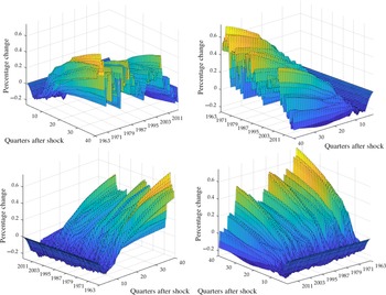
This section reports IRFs to explore the time-varying transmission of the immigration supply shock to the US macroeconomy and how immigration responds to the TFP and news shocks. I provide three-dimensional IRFs which plot the responses date by date. The x axis represents the after-training sample period from 1963Q1 to 2017Q4. The y axis is the 40-quarter forecast horizon. The z axis denotes the size of the responses. These IRFs are computed as responses of the specified variable to a one standard deviation shock at quarter t in the sample. Further, two-dimensional IRFs are displayed on selected major immigration policy dates. They are 1980Q1, 1986Q1, 1990Q1, 2004Q1, and 2010Q1, which correspond to the enactment of the Refugee Act, the IRCA, the IMMACT, the H1-B Reform Act, and Operation Streamline.
4.3.1 Effects of the immigration supply shock
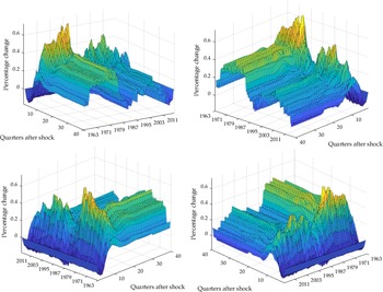
On ALP. Figure 3 plots the three-dimensional time-varying IRFs of ALP with respect to the immigration supply shock. Because of SR2, the immigration supply shock has no effect on ALP at impact. The IRFs show inverse hump-shaped paths with noticeable troughs around three to four quarters after the shock. At these horizons, the effect of an immigration supply shock on ALP is negative up to
 $-0.2$
percentage points but appears stable over the sample. The business cycle horizon and long-run responses of ALP with respect to an immigration supply shock exhibit substantial drift across the sample. The IRFs over the entire sample turn positive after five quarters and peak at the eighth quarter. The peak ranges from 0.1 to 0.7 percentage points. The IRFs of ALP mostly settle at a permanent higher level after about 16 quarters.
IRFs of ALP to an immigration supply shock, 1963Q1–2017Q4.
Notes: The 3D plots show the median responses of average labor productivity to an immigration supply shock across the entire sample. The sample period is 1963Q1–2017Q4. X-axis: quarters after shock; y-axis: magnitude of response (percentage change); z-axis: sample date. SVAR estimated with Model 1. Plots are rotated for viewability.

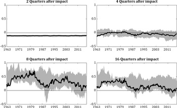
A few interesting results from Figure 3 are worth noting. First, the 1986 IRCA and 1990 IMMACT are important for understanding the dynamics of immigration and ALP. In the first half of the sample until the late 1980s, the immigration supply shock leads to an increase in ALP from the business cycle into the long run. The positive response begins to decline between 1985 and 1990 giving way to the diminishing responses in the second half of the sample. This finding is reinforced in Figure 4, which plots the IRFs of ALP at 2, 4, 8, and 16 quarters after the initial shock over the entire sample with 16–84% posterior tunnels. At the 8- and 16-quarter horizons, the pre-1990 responses are significantly larger than those of post-1990. Further, the negative short-run response of ALP to the immigration supply shocks is significant but short-lived. Figure 4 indicates that the median negative responses are indistinguishable from zero by the fourth quarter post-shock over the entire sample. This suggests new immigration behaves like an imperfect substitute to domestic labor in the short run and a complement in the long run.
IRFs of ALP to an immigration supply shock at selected horizons.
Notes: The solid (black) lines are median responses of average labor productivity to an immigration supply shock at 2, 4, 8, and 16 quarters after initial shock. Gray shaded areas are 16–84% posterior tunnels. X-axis: sample date; y-axis: magnitude of response (percentage change). SVAR estimated with Model 1.

The 1986 IRCA and 1990 IMMACT remain crucial episodes to the dynamics of immigration and other macroeconomic variables. The reason is twofold: (i) the 1986 IRCA ratified the largest nationwide amnesty (of irregular immigrants residing in the USA) to date, which likely altered immigration demographics such as education and skill level to a large extent; (ii) the 1990 IMMACT increased the overall immigration cap by 58%, most of which was family-based and employment-based visas that led to permanent residency. The IMMACT assumably changed immigration composition and expectation in family-based immigration.
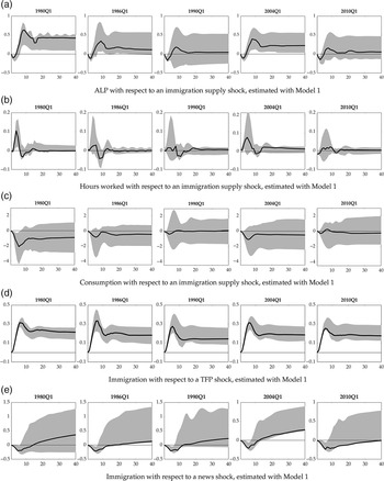
To further illustrate this point, Panel (a) of Figure 5 shows the two-dimensional IRFs of ALP to an immigration supply shock on the selected immigration policy dates with 16–84% error bands. The diminishing height of the ALP responses is evident throughout these immigration policy change dates. Around the 1990 IMMACT and the 2010 Operation Streamline, an immigration shock has a negative short-run and neutral long-run effect on ALP. Changes in immigration policy that drastically alter immigration composition correlate with the ambiguous response of ALP to immigration supply shock. Following up on the importance of immigration policy change, I also examine IRFs of ALP to an immigration supply shock at four quarters post each selected policy date (available in the Online Appendix). These IRFs display minimal qualitative and quantitative differences, if any, compared to their immigration policy date counterparts.
IRFs at selected immigration policy dates.
Notes: The solid (black) lines are median responses at selected immigration policy dates. Gray shaded areas are 16–84% posterior tunnels. X-axis: sample date; y-axis: magnitude of response (percentage change in (a), (c), (d), and (e), and log points in (b)). Selected dates are 1980Q1, 1986Q1, 1990Q1, 2004Q1, and 2010Q1.

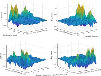
On Hours Worked. The IRFs of hours worked to an immigration supply shock are displayed in Figure 6 on the entire sample. The impact response of hours worked to an immigration supply shock, which is estimated according to Model 1’s identification, is near zero throughout the sample. This is because the structural impact coefficient of immigration on hours worked,
 $a_{23,t}$
, is small over the entire sample. The IRFs peak at the fourth quarter after initial shock and display large variation across the sample. Similar to the discussion earlier, the 1986 IRCA leading to the 1990 IMMACT is important to the dynamics of hours worked and immigration. Prior to 1990, an immigration shock increases log weekly working hours by up to 0.12 (or 1.13 h) by the fourth quarter post-shock. The average response post-1990 drops to around 0.03 (or 1.03 h). Over the business cycle horizons and in the long run, an immigration shock does not qualitatively or statistically affect hours worked.
IRFs of hours worked to an immigration supply shock, 1963Q1–2017Q4.
Notes: The 3D plots show the median responses of hours worked to an immigration supply shock across the entire sample. The sample period is 1963Q1–2017Q4. X-axis: quarters after shock; y-axis: magnitude of response (log points); z-axis: sample date. SVAR estimated with Model 1. Plots are rotated for viewability.

These IRFs suggest two prominent features of how immigration affects the labor market. According to the IRFs, hours worked responds to an immigration supply shock with a lag. The delayed effect of the immigration supply shock suggests frictions in the labor market. Next, the effect of the 1986 IRCA and 1990 IMMACT only pertains to the short run of around four quarters post-initial shock. Panel (b) of Figure 5 plots the IRFs of hours worked to an immigration supply shock at selected policy dates. Error bands indicate the peaks in the IRFs of hours worked around 1980 are statistically meaningful. However, there is large uncertainty about the effect of the immigration supply shock on hours worked after 1986.
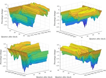
On Consumption. Figure 7 plots the three-dimensional IRFs of consumption to an immigration supply shock from 1963Q1 to 2017Q4. Although the contemporaneous response of consumption to an immigration supply shock is estimated according to the short-run identification of Model 1, the IRFs suggest near zero responses at impact over the entire sample. Consumption decreases on impact and in the short run with respect to an immigration shock. The trough of the median responses is around 6–8 quarters post-shock. Panel (c) of Figure 5, which plots the IRFs of consumption to an immigration supply shock at selected policy dates, suggests these short-run dynamics are quantitatively significant. Drifting height of the long-run responses is apparent with a shift at 1990Q1. The median long-run responses post-1990 settle near zero, while those prior to 1990 can be as low as
 $-2.5$
percentage points. The immigration supply shock generates a median long-run decline in consumption before 1990, but this effect becomes long-run neutral after 1990.
IRFs of consumption to an immigration supply shock, 1963Q1–2017Q4.
Notes: The 3D plots show the median responses of consumption to an immigration supply shock across the entire sample. The sample period is 1963Q1–2017Q4. X-axis: quarters after shock; y-axis: magnitude of response (percentage change); z-axis: sample date. SVAR estimated with Model 1. Plots are rotated for viewability.

These estimates suggest immigration has an adverse effect on consumption at least in the short run. A similar result is reported by Kiguchi and Mountford (Reference Kiguchi and Mountford2019). They argue the negative short-run effect is caused by an immigration-led increase in population that outpaces the growth in consumption. However, as Figure 7 suggests, the pre-1990 IRFs are at odds with their “catch-up” theory. I again point to the importance of the 1986 IRCA and 1990 IMMACT. After these policy changes, the numerator was able to rise faster in the medium- to long-run, which allows the “catch-up” and alleviates the negative effects of immigration on consumption.
4.3.2 Effects of the macroeconomic shocks
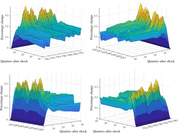
TFP Shock on Immigration. Figure 8 contains plots of the three-dimensional IRFs of immigration with respect to a TFP shock. Recall identifying restriction SR1 that immigration responds to macroeconomic fluctuations only with a lag. Over the sample, the hump-shaped immigration responses peak at the eighth quarter and settle at a permanently higher level after 16 quarters. The drift in the IRFs is mostly at peak, which displays co-movement with changes in immigration policy. For instance, a large dip in the peak response of immigration to a TFP shock coincides with the 1986 IRCA and 1990 IMMACT.
IRFs of immigration to a TFP shock, 1963Q1–2017Q4.
Notes: The 3D plots show the median responses of immigration to a TFP shock across the entire sample. The sample period is 1963Q1–2017Q4. X-axis: quarters after shock; y-axis: magnitude of response (percentage change); z-axis: sample date. SVAR estimated with Model 1. Plots are rotated for viewability.

Panel (d) of Figure 5 displays the IRFs of immigration to a TFP shock with error bands. These plots suggest the positive effects of a TFP shock on immigration is quantitatively meaningful at the business cycle frequencies and in the long run. Further, the decline in the height of the responses around 1990 is visible. This evidence reinforces the importance of the 1990 IMMACT and indicates these changes in immigration policy can suppress the effect of a TFP shock on immigration.
News Shock on Immigration. I plot the three-dimensional IRFs of immigration to a news shock in Figure 9. In the short run, immigration declines with respect to a positive news shock. The responses turn positive over the business cycle horizons and stay permanently higher during most sample periods. The inverse hump shapes of the IRFs are clear in Panel (e) of Figure 5 on selected immigration policy dates. However, the long-run effect of a news shock to immigration appears to be neutral in several IRFs (1986Q1, 1990Q1, 2010Q1). It is well documented in the news literature that the short-run negative labor response is consistent with standard macroeconomic theory of inter-temporal substitution. The shapes of these IRFs are in line with the consensus from the news literature that macroeconomic variables follow the predicted movements in TFP responses, for example, Barsky and Sims (Reference Barsky and Sims2011).
IRFs of immigration to a news shock, 1963Q1–2017Q4.
Notes: The 3D plots show the median responses of immigration to a news shock across the entire sample. The sample period is 1963Q1–2017Q4. X-axis: quarters after shock; y-axis: magnitude of response (percentage change); z-axis: sample date. SVAR estimated with Model 1. Plots are rotated for viewability.

4.4 Forecast error variance decompositions
The time-varying structure of the SVARs allows the composition of forecast errors to vary date by date. The reported forecast horizons are 2, 4, and 20 quarters and the long run on selected immigration policy dates. Similar to the IRFs, the dates are 1980Q1, 1986Q1, 1990Q1, 2004Q1, and 2010Q1.
Table 3 reports the FEVDs of ALP, immigration, consumption, and the term spread with respect to an immigration supply shock. First, the immigration supply shock is responsible for around 30% of the short run (2–4 quarters post-shock) fluctuations in consumption and the term spread. The importance diminishes to 20% or lower in the long run. This indicates that the importance of the immigration supply shock to the US macroeconomy pertains to the short run and business cycle horizons. The contribution of an immigration supply shock to ALP and hours worked (omitted) is less than 15% and fluctuates minimally across the sample and over the forecast horizons.
FEVDs with respect to immigration supply shock

Notes: Results based on TVP-SV-SVAR estimated with Model 1. Selected immigration policy dates correspond to the Refugee Act of 1980, the IRCA of 1986, the IMMACT of 1990, the H1-B Act of 2004, and Operation Streamline of 2010. The long-run (
 $\rightarrow{\infty}$
) FEVD is defined as a forecast horizon of 40 quarters. The FEVDs of hours worked and posterior tunnels for all FEVDs can be found in the Online Appendix.
The immigration supply shock accounts for around 40% of the fluctuations of immigration from the short run into the business cycle frequencies. The dominance of immigration by its own shock is stable over the sample. This indicates the decision to immigrate is one of the most important sources in explaining variations of immigration at all horizons.
TFP, labor demand, and news shocks are also important for explaining the variation in immigration. Table 4 displays the FEVDs of immigration with respect to the macroeconomic shocks at selected horizons and immigration policy dates. The labor demand shock contributes the second largest error variance share to the variations of immigration at about 35% in the short run and business cycle frequencies with small variations over the sample. In the long run, the labor demand shock becomes a large source of immigration fluctuations. The TFP shock accounts for 18% of the fluctuations in immigration in the short run, but this importance diminishes after four quarters. In contrast, the news shock contributes to the variation of immigration only at the business cycle frequencies and in the long run. This finding suggests that the TFP shock plays a role in explaining the short-run variations in immigration, while the importance of the news shock only pertains in the long run.
Immigration FEVDs with respect to macroeconomic shocks

Notes: Results based on TVP-SV-SVAR estimated with Model 1. Selected immigration policy dates correspond to the Refugee Act of 1980, the IRCA of 1986, the IMMACT of 1990, the H1-B Act of 2004, and Operation Streamline of 2010. The long-run (
 $\rightarrow{\infty}$
) FEVD is defined as a forecast horizon of 40 quarters. The Online Appendix provides posterior tunnels for all FEVDs.
5 Conclusion
This paper studies the dynamic relationship of immigration and the US macroeconomy from 1953Q1 to 2017Q4. I estimate structural VARs with time-varying intercepts and slope parameters and disturbances subject to SV. The structural shocks are identified with a combination of short- and long-run restrictions on ALP, hours worked, immigration, consumption, and the 10-year Treasury yield to 3-month Treasury bill spread. A Bayesian model selection exercise is used to find the identification that is favored by the data. This identification restricts immigration to respond only to its own supply shock at impact, while ALP responds to the immigration supply shock in the long run.
I find important time-varying dynamics between immigration and the US macroeconomy. The IRFs suggest an immigration supply shock increases ALP at the business cycle horizons and in the long run. The IRFs of hours worked to an immigration supply shock also rise at the business cycle horizons. Furthermore, shocks to the state of the macroeconomy affect immigration. A TFP shock raises immigration at the business cycle horizons, while the positive effect of a news shock on immigration only pertains in the long run. However, these IRFs are dependent on changes to US immigration policy, especially the IRCA of 1986 and the IMMACT of 1990.
TFP and news shocks play an important role in explaining the variations of immigration in the short and long run, according to the FEVD results. The immigration supply shock explains about one-third of the fluctuations in consumption and the term spread at the business cycle frequency. I interpret this evidence to mean that immigration has been relevant to the US macroeconomy since 1963.
My estimates show that the responses of immigration to the identified shocks are heavily dependent on the immigration policy regime. This suggests future research should focus on the impact of immigration conditional on existing immigration policy and the state of the macroeconomy. Another useful research issue is to identify an immigration policy shock and estimate its effect on immigration supply and real economic activity. I leave these questions for future research.
Supplementary Material
To view supplementary material for this article, please visit http://dx.doi.org/10.1017/S1365100521000298.