




No CrossRef data available.
SOME LIMIT THEORY FOR AUTOCOVARIANCES WHOSE ORDER DEPENDS ON SAMPLE SIZE
Published online by Cambridge University Press: 04 August 2003
Abstract
In this paper we provide some weak convergence results for sample statistics of the product of a variable with its kth-order lag. We assume the variable is a stationary vector that can be represented by linear process, and the lag length k is allowed to be a function of the sample size. Employing the Beveridge–Nelson decomposition, we derive a new functional central limit theorem for this situation and establish related stochastic integral convergence results. We then consider the behavior of associated long-run variance estimators and also extend our analysis to the case where the sample statistics are based on regression residuals. We illustrate the potential range of application of these techniques in the context of (i) testing for I(0) versus I(1) behavior and (ii) estimation and testing in a heteroskedastically cointegrated regression model.We thank the co-editor and the referees for helpful comments on earlier drafts.
Information
- Type
- Research Article
- Information
- Copyright
- © 2003 Cambridge University Press
1. INTRODUCTION
The aim of this paper is to provide some weak convergence results for sample statistics of the process {ζtζt−k′}, where ζt is a weakly stationary vector linear process. The innovation lies in the fact that here k is a function of the sample size T such that k → ∞ as T → ∞. Standard asymptotic results, such as those on the (functional) central limit theorem ((F)CLT), stochastic integral convergence (SI), and long-run variance estimation (LRV), do not apply in the case where k grows with T, and so we provide extensions of these standard tools to deal with the new situation.
To motivate the need for such results, Section 2 presents examples of simple testing and estimation problems where such convergence results are directly relevant. Our approach to deriving these results relies on a linear process assumption for ζt, which we combine with the Beveridge–Nelson (BN) decomposition as advocated by Phillips and Solo (1992) to obtain new limit theorems. The algebra of the BN decomposition is similar to Phillips and Solo (1992), but, as we demonstrate, with k → ∞ the resulting martingale difference approximation to ζtζt−k′ differs in important aspects from the standard case in which k is fixed. The specific assumptions on ζt and the details of the BN decomposition of ζtζt−k′ are given in Section 3. Section 4 contains the main theorems. The FCLT is derived in Section 4.1, and some associated stochastic integral results are derived in Section 4.2. To facilitate the practical implementation of the FCLT, the asymptotic properties of certain long-run covariance matrix estimators are considered in Section 4.3. In Section 5 we then return to the testing example of Section 2.1 and show how the theorems introduced accommodate the fact that k depends on T and yield asymptotic normality of the test statistic. However, in many applications residuals have to be used to perform analyses as the data themselves require detrending in some way, and in Section 6 we demonstrate that our results apply to regression residuals. It follows that the test presented in Section 2.1 is valid in these circumstances too. Section 7 then examines how the test procedure performs in practice, using Monte Carlo methods. Section 8 continues to illustrate the way the theorems of Section 4 are utilized by revisiting the estimation example of Section 2.2. Finally, the proofs of the theorems are given in Section 9.
2. MOTIVATION
Although our results should be of general interest, this section provides two specific examples where they apply directly. The first example involves testing for I(0) versus I(1) in a univariate time series. We suggest a very simple “stationarity” test based on the lag k autocovariance and use the FCLT to show that it has a standard normal distribution under the I(0) null. Thus, we provide an additional test to those already proposed by, inter alia, Kwiatkowski, Phillips, Schmidt, and Shin (1992), Saikkonen and Luukkonen (1993), and Leybourne and McCabe (1994). The second example concerns estimation and testing in the heteroskedastic cointegration framework developed by Hansen (1992a) and recently generalized by Harris, McCabe, and Leybourne (2002). We show that ordinary least squares (OLS) estimation in this model is inconsistent, but consistency, together with asymptotic normality, can be obtained via an estimator that exploits the FCLT and SI results developed here. To assist the flow of ideas, proofs of the asymptotic results appearing in these examples are treated after the theorems have been introduced.
2.1. Testing I (0) versus I (1)
Let the observed time series zt be generated by the AR(1) process

where the disturbance term εt is white noise with variance σ2. Suppose we wish to test the parametric composite I(0) null hypothesis 0 ≤ ρ < 1 against the I(1) alternative ρ = 1. Consider the sample autocovariance based on observations t = 1,2,…,T:

For ρ < 1 we have the standard result

so that, for k small relative to T,

Whereas for ρ = 1,

so, for k small relative to T,

The differing orders of magnitude of E(S) in the two cases allow S to form the basis of a consistent test to distinguish between them. As in the case of the likelihood ratio approach, a problem arises because the asymptotic distribution of S, under the composite null, will not be free of parameters as, from (2), it will depend on ρ for any fixed k . However, now suppose that we allow k to increase simultaneously with T such that k = k(T) = o(T). Then it is clear from (2) that E(S) will converge to zero at a rapid rate, eliminating any dependence of E(S) on the parameter ρ. Because, as is seen from (3), S will still be divergent under ρ = 1, it provides the basis for a test that is consistent. It is also clear that a CLT is needed that can be applied to quantities like S. Standard techniques do not apply here as zt zt−k is a function of k that is in turn a function of T.1
We generally suppress the dependence of k on T to economize on notation.
Our approach to this problem is to construct an approximating martingale difference array for zt zt−k via the BN decomposition. This is the content of Theorem BN in Section 3. Moreover, even though we allow k = k(T) = o(T) in accordance with Assumption K in Section 3, a martingale central limit theorem may still be applied to the approximating martingale for S. In addition, Lemma 4 in Section 4 shows that the approximation error is negligible. Specifically, we find using Theorem FCLT in Section 4 that

To provide S with a distribution that is independent of parameters, we also need a consistent estimate of the variance of the limit distribution. This is accomplished by means of a long-run variance estimator as in Theorem LRV in Section 4. Letting

denote the LRV estimator, we find

Thus, the device of letting k = k(T) → ∞ solves the problem of testing a composite null when the conditions of Theorems FCLT and LRV hold.
In many cases zt is not observed directly but is the disturbance term in a regression with deterministic variables (which can include polynomial trends, structural breaks, etc.); nevertheless (4) still holds when S* is constructed from the OLS residuals from such a regression model. The details are given in Section 6.
2.2. Heteroskedastic Cointegration
Harris et al. (2002) consider a model that generalizes the heteroskedastically cointegrated regression model of Hansen (1992a). In its bivariate form, which we study here for illustrative purposes, the model can be written

where εy,t, εx,t, ηt, vy,t, and vx,t are independent stationary zero-mean disturbance terms and πy and πx(≠ 0) are constants.2
This independence assumption is made here only to elaborate the most pertinent features of the model within the simplest possible framework. A rather more general setup is given in Harris et al. (2002).

where

and vt = vy,t − βvx,t and εt = εy,t − βεx,t.
The processes yt and xt are said to be individually heteroskedastically integrated, and are mutually heteroskedastically cointegrated. Hansen's model is a special case of this one that assumes πx,t = πx, such that xt is I(1), rather than being heteroskedastically integrated, and so the model is “unbalanced,” as yt is still heteroskedastically integrated. He shows that OLS estimation of β is consistent in that case. However, under the more general specification given previously we can easily show that, for the OLS estimator

,

so that OLS is inconsistent because E(πx,t vt) ≠ 0. Instead, consider an estimator of the form

This estimator was introduced in Harris et al. (2002). Under Assumptions LP and K, which follow, we can show that

In the numerator we are required to deal with

, and thus we need results on convergence to stochastic integrals when the increment process is multiplicative involving lag k → ∞. However, this sort of integral convergence needs a FCLT to be available for the partial sum of the increment process (and indeed for the process wt). In fact, because there are two sums involved we need joint convergence of these increment processes and the rest of the variables in the model; i.e., we are required to deal with convergence of the multivariate process (ζt′,vec(ζtζt−k′)′)′ where ζt = (εy,t,εx,t,ηt,vt,vx,t)′. Theorem FCLT gives a general result of this form that applies when the variables are generated by linear processes, whereas Theorem SI in Section 4 deals with integral convergence.
Specifically, we show

where W and H are independent Brownian motions. Also, given that

we find

Hence, conditional on W, the asymptotic distribution of

is normal. With a suitable heteroskedasticity and autocorrelation consistent (HAC) variance estimator, this result permits construction of hypothesis tests for β using a standard normal distribution.
3See Harris et al. (2002) for details.
Although the illustrative examples given previously are, respectively, univariate and bivariate in the observable variables, they can both be generalized quite naturally to multivariate situations. For example, a vector generalization of S* can easily be constructed to provide a test of I(0) against I(1), and Harris et al. (2002) explicitly consider the case where xt is a vector process. Because of this, together with the fact that the quantities of interest are multivariate in the observed and disturbance variables together, the results presented in the remainder of this paper purposely address the vector case. The next section gives details of the BN decomposition, which is then used to provide a martingale approximation to a linear process.
3. THE BEVERIDGE–NELSON DECOMPOSITION
For any matrix A let

and suppose that a vector time series ζt satisfies the following linear process assumption.
Assumption LP. Let ζt be an n × 1-dimensional vector linear process generated by

where

and Cj (n × n) and ξt (n × 1) satisfy

We use the BN decomposition to provide a martingale approximation for ξt to facilitate distribution theory and the fact that k depends on T. See Section 5 for an example of how this works. For r = 0,±1,±2,… define the lag polynomials
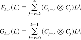
and Gk,r = Gk,r(1). The BN decomposition of the vector process

is given by the following theorem.
THEOREM 1 (BN). If ζt satisfies Assumption LP then the BN decomposition of Zk,t is given by

where

are partitioned conformably with Zk,t and are given by

where

is a martingale difference sequence composed of

and the remainder terms are

Theorem BN, in its algebraic detail, is essentially a multivariate version of the BN decomposition for ζt and ζtζt−k given by Lemma 2.1 and equation (28), respectively, of Phillips and Solo (1992). A main difference between Theorem BN and the Phillips and Solo results is that the role of rk,t differs depending on whether k → ∞ or k is fixed. In this paper, where k → ∞, rk,t is a remainder term because it disappears in all of the limit theorems. This is a result of the following lemma, which is proved in Section 9.
LEMMA 2. Under Assumption LP,

.
That is, if k → ∞ at least as fast as T1/α then the sum of squares of rk,t disappears asymptotically. This lower bound on the rate of increase of k is exactly that imposed in Theorem FCLT to obtain an FCLT for Zk,t. It is stated as an assumption for future reference.
Assumption K. Let k → ∞ as T → ∞ such that k/T → 0 and k/Tβ [nrarr ] 0, 1/α ≤ β < 1.
If k is fixed, as in Phillips and Solo (1992), then rk,t does not disappear in the asymptotics. For example

is nonzero in general for fixed k, but E(vec ζtζt−k′) → 0 if k → ∞. It follows that the approximating martingale difference for limit theorems for vec ζtζt−k′ with fixed k is

where Fk,k−i = Fk,k−i(1), which is the same as that reported by Phillips and Solo but in different notation. Therefore, although the algebra of the BN decomposition is the same for all k, there are important differences in the asymptotics between the case of k fixed and k → ∞.
A difficulty in obtaining limit theorems for ζtζt−k′ with k → ∞ is that the strength of the intertemporal dependence in ζtζt−k′ is a function of T via k. The utility of the BN decomposition is that even in this case it yields an approximating martingale difference array mk,t for ζtζt−k′, and the effect of k is relegated to the constant matrices Gk,k−j. These constant matrices only have an effect on the variance Ω22 = limk→∞ E(mk,t mk,t′); see Theorem FCLT. The next section uses this decomposition to prove some results that are useful in conducting asymptotic analyses of product processes.
4. THEOREMS
This section provides a set of tools for analyzing ζtζt−k′ processes indexed by k(T). An invariance principle and an associated lemma are given in the Section 4.1, and this is followed by some results on stochastic integral convergence. The Section 4.3 deals with long-run variance estimation.
4.1. The Functional Central Limit Theorem
As before let

THEOREM 3 (FCLT). Under Assumptions LP and K

where B = (B1′,B2′)′ is n2 + n-dimensional Brownian motion partitioned conformably with Zk,t and has covariance matrix

where

.
The FCLT showing the weak convergence of partial sums of the marginal linear process ζt to B1 is standard. The new result consists of the sufficient conditions for the FCLT for ζtζt−k′ with k → ∞ and its asymptotic independence of ζt.
The proof of Theorem FCLT is immediate from application of Theorem BN to Zk,t, followed by Lemma 4.
LEMMA 4. Under Assumptions LP and K,

The details of the proof of Lemma 4 are given in Section 9. Part (i) follows from a martingale array FCLT, and part (iii) is a standard BN decomposition remainder term. Part (ii) follows from Lemma 2 and leads to the imposition of Assumption K in Theorem FCLT.
Theorem FCLT can be contrasted with Keenan (1997). Keenan's underlying process is strictly stationary and strong mixing, whereas we assume a linear process with bounded moments that is not strictly stationary or mixing. Keenan is specifically interested in joint (uniform) weak convergence for the set of centered autocovariances

for appropriate m(T) → ∞ as T → ∞ so that the limit distribution is multivariate normal. That is, he provides joint distributions, whereas (4) only applies to a single autocovariance at lag k. The multivariate (and uniform) nature of Keenan's results restricts the choice of m(T) and in particular excludes the case where m(T) = O(T1/2). This has implications for the centering of the statistic of interest. For example, because our univariate CLT allows for k(T) = O(T1/2) the statistic in (4) need not be centered in the numerator because T1/2E(zt zt−k) → 0 under our assumptions and hence (4) is more relevant to the current hypothesis testing problem. In addition, (4) includes the estimated variance

and cases where residuals are used.
The following corollary to Theorem FCLT is useful in the theory of estimation of heteroskedastically cointegrating vectors (see Harris et al., 2002; and Section 2.2).
COROLLARY 5. Let ζt(μ) = μ + ζt where μ is an n × 1 constant vector. Under Assumptions LP and K

where B3(τ) = μ [otimes ] B1(τ) + B2(τ).
This follows because vec(ζtζt−k(μ)′) = μ [otimes ] ζt + vec(ζtζt−k′) and from the application of Theorem FCLT. Clearly the same result holds for ζt(μ)ζt−k′.
4.2. Stochastic Integral Convergence
This section gives conditions for the convergence to a stochastic integral of a statistic that has the form

where ζt satisfies Assumption LP, ζt(μ) is defined in Corollary 5, Q is a fixed m × n2 matrix, and UT,t is a p × m matrix process. Results for ζtζt−k′ as the increment process follow by setting μ = 0. The presence of the fixed matrix Q is not important for the general result but proves to be convenient in applications.
A general solution for the limit of (10) has not been found. Using Theorem BN gives the BN decomposition

for which the following theorem is proved. Define MT,[Tτ] = T−1/2 Σ[Tτ] mk,t(μ) to be the partial sum process of mk,t(μ).
THEOREM 6 (SI). If Assumptions LP and K hold and

then

where BQ(τ) = QB3(τ) and

Details of the proof are given in Section 9. Theorem 2.1 of Hansen (1992b), which shows convergence to a stochastic integral with a martingale difference array increment process, is used for (12), and Lemma 2 implies (13). Thus (10) weakly converges to a stochastic integral of the form ∫UdBQ plus another term that is the limit of

. This extra term could be zero, a constant, or a random limit depending on the structure of the process UT,t and its relationship to ζt.
Theorem SI is complementary to the results of Phillips (1988), who derives stochastic integral convergence results where the increment process is a linear process such as ζt.
4.3. Long-Run Covariance Matrix Estimation
Estimators of long-run covariance matrices related to ζtζt−k′, such as Ω22, may be required in applications. This section presents some results for kernel-based estimators of the form

where at is any vector time series, λ(.) is the kernel, l is the bandwidth parameter, and

In general, consistency of a long-run covariance matrix estimator is sufficient for statistical inference. The next theorem gives conditions for

to be consistent when applied to ζtζt−k(μ)′ with k → ∞.
THEOREM 7 (LRV). If Assumptions LP and K hold and
(i) l → ∞ as T → ∞ such that l = o(kα/2),
(ii) 0 ≤ λ(x) ≤ 1 for |x| ≤ 1, λ(x) = 0 for |x| ≥ 1, and λ(0) = 1,
(iii) λ(x) is even, continuous, and |λ(x) − λ(y)| ≤ C|x − y| for some constant C, then

The condition that the bandwidth satisfy l = o(kα/2) should not prove restrictive in applications. It implies that l = o(Tαβ/2) where αβ ≥ 1 by assumption. This allows the usual mean square error–optimal choices of l (→ ∞), including l = O(T1/3) for the Bartlett kernel and l = O(T1/5) for the various quadratic kernels.
5. Testing I (0) versus I (1) Revisited
We now continue with the testing example of Section 2.1 and illustrate how the theorems just introduced apply. Let Assumption K hold and note that for ρ < 1, Assumption LP applies to zt in (1). The BN decomposition gives

where

with

where εt is as previously defined. Now, letting

be all the information up to time t − 1,

and so mk,t is a martingale difference with the convenient property that the effect of k is relegated to the constant terms Gk,k−j. The variance of the martingale only depends on these Gk,k−j. This is how the BN decomposition effectively solves the problem that k depends on T. Applying Theorem FCLT and Lemma 4 gives

where

. It is then straightforward to show

Finally, that

follows directly from Theorem LRV.
In many cases zt will not have zero mean and the test will have to be applied to regression residuals. The next section gives conditions under which our theorems are valid when computed using residuals from regression models.
6. REGRESSION EFFECTS
Suppose, quite generally, that

are the OLS residuals

where xt is a vector of deterministic regressors such that

uniformly in τ for some matrix DT and

For example, if xt = (1,t)′ then DT = diag(1,T) and X(τ) = (1,τ)′.
The following theorem shows the extent to which Theorems FCLT, SI, and LRV are unaffected by the replacement of ζt by

.
THEOREM 8 (RES). Under Assumptions LP and K and (14)–(16)
(i)

(ii) under the conditions of Theorem SI

(iii) under the conditions of Theorem LRV with l = o(T1/2)

Part (i) shows that Theorem FCLT continues to hold for

, i.e.,

where B2 is the Brownian motion defined in Theorem FCLT. This is in contrast to the FCLT for

, which is well known to be affected by preliminary regressions such as (14). For example, if xt is a constant then

converges weakly to a Brownian bridge with covariance matrix Ω11. Corollary 5 generally does not apply as stated when ζt is replaced by

because it relies on the FCLT for ζt and also ζtζt−k′.
Part (ii) shows that Theorem SI remains valid when the increment process ζtζt−k′ is replaced by

. However, it does not apply when ζtζt−k(μ)′ is replaced by

for the same reason that Corollary 5 does not apply when residuals are used.
Part (iii) shows that Theorem LRV applies to

. Our applications involving μ do not require that it be observable (see Sections 2.2 and 8), so consideration of the estimation of μ is not required. The extra condition on l should not prove restrictive in practice.
The nature of the regressors allowed for in Theorem RES makes the result well suited to the testing application (see Sections 2.1 and 5). This means that the asymptotic normality result (4) continues to hold when S* is calculated using residuals from regression models with deterministic regressors that include polynomial trends, and so on. The theorem does not apply to the heteroskedastic cointegration model of Section 2.2 because stochastic regressors are involved. The results for long-run covariance matrices for heteroskedastically cointegrating regressions are considerably more complicated than Theorems LRV and RES(iii), and are treated in detail in Harris et al. (2002).
7. Testing I(0) versus I(1): Some Monte Carlo Evidence
In this section we present a small Monte Carlo simulation exercise to show how the test S* may perform in finite samples, focusing on the effects of different choices of k. Assumption LP(ii), at its most lenient, implies that we may set α = 2. For this choice, Assumption K then requires that k → ∞ at least as fast as T1/2. In this exercise we therefore select three compliant values: k = [T1/2], [T7/12], [T2/3] .
4Here [x] denotes the integer part of x.

. Then S* is constructed as

where we use the Bartlett kernel for λ(.) in

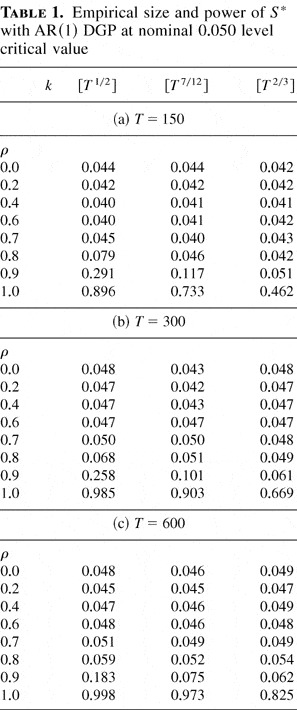
, setting the bandwidth parameter l = [T1/3] , a fairly typical value in applications of this kind and one that is compatible with our chosen values for k (see Theorem LRV(i)). Table 1 gives empirical size of S* under the I(0) null (ρ < 1) and power under the I(1) alternative (ρ = 1) for sample sizes T = 150, 300, 600. The entries are upper-tail empirical rejection probabilities of the I(0) null at the nominal 0.050 level critical value of the asymptotic N(0,1) distribution. These are based on 10,000 replications.
Empirical size and power of S* with AR(1) DGP at nominal 0.050 level critical value

The main features of Table 1 are fairly transparent. Under the null, when ρ is small, S* is approximately correctly sized irrespective of how k is chosen. In small samples, however, k = [T1/2] leads to oversizing when ρ is close to 1. This effect is evident, but much less pronounced, for [T7/12] and absent for [T2/3] . Recalling (2), this is pretty much as we might expect because the mean effect, here a rightward shift away from the origin, diminishes more quickly the faster k grows. Any oversizing problems with the lower rates of increase of k are largely ameliorated as the sample size increases and the asymptotics start to gain hold.
As regards test power (issues of oversizing notwithstanding) for a given sample size this is inversely related to rate of increase of k, dropping quite sharply when k = [T2/3] . A partial explanation for this is simply that a higher rate involves the sacrifice of a larger number of sample observations and this may make a significant difference when T is relatively small. It is clear however that, for each of the different rates of increase of k studied here, S* is consistent. Thus, the choice of k needs to be made keeping this size/power trade-off in mind. If one is prepared to take the view that in terms of relative size performance k = [T7/12] has more in common with k = [T2/3] than k = [T1/2] and, at the same time, that in terms of relative power performance it has more in common with k = [T1/2] than k = [T2/3] then there appears to be at least some justification for making [T7/12] the operational choice of k. We recognize, however, that this choice issue really warrants a rather more rigorous analysis than has been attempted here.
8. HETEROSKEDASTIC COINTEGRATION REVISITED
Let Assumption K hold and Assumption LP apply to the vector ζt = (εy,t,εx,t,ηt,vt,vx,t)′ in the model (5), where these disturbances are as specified in Section 2.2. First, to show (6) note

where en is an n × 1 vector with element n equal to 1 and 0's elsewhere. Now an application of Theorem FCLT applied to the marginal process ηt and the mapping theorem gives UT,[Ts] = T−1w[Ts]2 ⇒ U(s) ≡ W(s)2 whereas Corollary 5 gives

where B3(τ) = μ [otimes ] B1(τ) + B2(τ). Theorem SI, in conjunction with (19), which follows, then shows that

where H(s) ≡ πB1(τ) + B2(τ) with B1(τ) being the limit Brownian motion associated with vt and B2(τ) that of vt vx,t−k. To show (7) write

because E(vx,t vx,t−k) → 0. The numerator (17) needs to be combined with the denominator (18) to give the distribution of

in (8). Theorem SI gives more than just the convergence of (17); it also gives joint convergence of the sum with UT,[Ts] = T−1w[Ts]2, and because

the mapping theorem yields (8). So combining the numerator and the denominator gives the distribution of

.
It remains to deal with the remainder term

where

being the component of the linear process that corresponds to the variable vx,t with Ci,x being the associated coefficients. By (13) the term involving rk,t is negligible. Note that

. Now,

behaves intuitively like the stochastic integral of T−1wt−12 with respect to

, except for the fact that this latter term is overdifferenced and hence the distribution of its partial sum process is degenerate. This overdifferencing induces a complex negative correlation structure in

such that it too is overscaled and hence converges in probability to zero. The computations to verify this are similar to those of Lemma 9 of McCabe, Leybourne, and Harris (2002). That

follows by similar arguments. Thus

9. PROOFS
Lemma 9 gives some summability results for the lag polynomial coefficients derived in Theorem BN.
LEMMA 9. If Assumptions LP and K hold then

Proof of (i). Assumption LP implies

. Thus

. █
Proof of (ii). Write

and apply equation (2) of Lemma 2.1 of Phillips and Solo (1992) with p = 2. █
Proof of (iii). Using some expressions from the proof of Theorem BN, write

The first term is bounded by

the second term is bounded by

and the third term is bounded by

These three bounds are finite under Assumption LP(ii) and are clearly uniform in k. █
Proof of (iv). Write

Under Assumption LP(ii),

. █
Proof of (v). Write

and this bound is finite under Assumption LP(ii). █
9.1. Proof of Theorem BN
The BN decomposition of ζt is standard:

To obtain the BN decomposition for ζtζt−k′, first write

Then

and

For i = 1

whereas applying the BN decomposition to Gk,k−i(L) for each i = 2,…,k − 1 gives

Note this latter expression for Gk,k−i(L) holds for all i = 1,…,k − 1. For i ≥ k,

Thus, for all i,

This gives

Note that

is a martingale difference sequence. █
9.2. Proof of Lemma 2
By Markov's inequality

for any ε > 0, and

where the last line follows by the matrix Cauchy–Schwarz inequality tr A ≤ n(tr A′A)1/2 = n∥A∥ where A is n2 × n2. Nonzero expectations arise for the pairs of indexes (i = q,j = p), (i = j,q = p) and (i = p,q = j). These three terms are

by Lemma 9(i), and

and

Thus E(∥rk,t∥2) = o(k−α), and substitution in (20) proves the lemma. █
9.3. Proof of Lemma 4
Proof of (i). A vector FCLT for the martingale difference array Mk,t = (m0,t′,mk,t′)′, such as Theorem 27.17 of Davidson (1994), requires

To show (a), consider first

Then

To complete (a), a weak law of large numbers is required to show that

Under Assumption LP(iv)–(vi)

. Next consider

. Note that this term has zero expectation, so

where

Thus the first term in (21), (i.e., s = 0), is O(T−1) by Lemma 9(iv), whereas the second term satisfies

which is similarly O(T−1) by Lemma 9(iv). Thus (21) disappears, and hence

. Last consider

. The approach is to show that

as T → ∞. Now

so

where Mn = In [otimes ] Kn [otimes ] In and Kn is the commutation matrix (see Magnus and Neudecker, 1988, p. 47). Then ∥var(vec mk,t mk,t′)∥ is given by

where c0 = max(κ2 + ∥Σ∥4,nκ∥Σ∥2), so

Now using

the s ≥ 1 lag autocovariance of vec mk,t mk,t′ is

Thus

where c1 = n2κ∥Σ∥2. Summing over s ≥ 1 gives

by Lemma 9(iv) and

because

Substitution of (24) and (25) in (23) gives

Thus combining (22) and (26) gives

as required.
To show (b), write

because E [(Mk,t′Mk,t)2] < ∞, again using Assumption LP(vi). █
Proof of (ii). Applying the triangle and Cauchy–Schwarz inequalities gives

and applying Lemma 2 gives the result. █
Proof of (iii). First write

For any t

and similarly

because nonzero expectations arise only when i = p and j = q in the first line. Thus, by Lemma 9(ii) and (iii),

uniformly in t and k. Hence

uniformly in k. █
9.4. Proof of Theorem SI
Theorem 2.1 of Hansen (1992b) applies to show (12). That is, (UT,[Tτ],Qmk,t(μ)) ⇒ (U(τ),BQ(τ)) and from the proof of Lemma 4(i)

so

.
To show (13) write

and, using Lemma 2, this is op(T1/2k−α/2). █
9.5. Proof of Theorem LRV
Using (11):

The limit follows from

where the law of large numbers was proved for Lemma 4(i). All other terms in (27) can be shown to disappear.
For j > 0,

by the martingale difference property of mk,t(μ), and

Thus

Next for any j ≥ 0

by Lemma 2, so

which disappears provided l increases more slowly than O(kα/2), as required by condition (i) of the theorem. Terms involving T−1 Σ r1k,t r1k,t−j′ disappear similarly at rate op(k−αl).
It remains to consider the terms involving

. For example, the terms involving cross-products of

are

and straightforward rearrangements give

The third term clearly disappears as T → ∞, and using that

gives that the first term satisfies

because

. Similarly the second term can be shown to disappear. This approach applies for all terms involving

. █
9.6. Proof of Theorem RES
Proof of (i). First write

Because supt≤T∥DT−1xt∥ = O(1) by (15), the second term of (28) disappears uniformly in τ provided

, where

Therefore, in view of (16), it is required to show that

converge in probability to zero and that

. The details are given for the first of these, with the other two following similarly. Write

Now

and

Thus (29) is O(T−1). Moreover, it is uniform in τ. Thus

. █
Proof of (ii). Write

The first term can be written

which disappears because the first term is Op(T−1/2). The second term in (30) disappears similarly. The third term can be written

By condition (ii) of Theorem SI,

, so this third term also disappears.
Proof of (iii). It is convenient to write

where, for

. First write

Because

where

there are a total of 15 product terms to insert in (31). We give the details for one of these terms, and the others follow in the same way. Consider

:

which disappears by condition (i) of Theorem LRV. The last line uses the fact that

. █
References
REFERENCES
Davidson, J.
(1994)
Stochastic Limit Theory.
Oxford, UK:
Oxford University Press.
Hansen, B.E.
(1992a)
Heteroscedastic cointegration.
Journal of Econometrics
54,
139–158.Google Scholar
Hansen, B.E.
(1992b)
Convergence to stochastic integrals for dependent heterogeneous
processes.
Econometric Theory
8,
489–500.Google Scholar
Harris, D.,
B.P.M. McCabe, &
S.J. Leybourne
(2002)
Stochastic cointegration: Estimation and inference.
Journal of Econometrics
111,
363–384.
Available at www.economics.unimelb.edu.au/dharris.Google Scholar
Keenan, D.M.
(1997)
A central limit theorem for m(n) autocovariances.
Journal of Time Series Analysis
18,
61–78.Google Scholar
Kwiatkowski, D.,
P.C.B. Phillips,
P. Schmidt, &
Y. Shin
(1992)
Testing the null of stationarity against the alternative of a unit
root: How sure are we that economic time series have a unit root?
Journal of Econometrics
54,
159–178.Google Scholar
Leybourne, S.J. &
B.P.M. McCabe
(1994)
A consistent test for a unit root.
Journal of Business and Economic Statistics
12,
157–166.Google Scholar
Magnus, J.R. &
H. Neudecker
(1988)
Matrix Differential Calculus with Applications in Statistics and
Econometrics.
New York:
Wiley.
McCabe, B.P.M.,
S.J. Leybourne, &
D. Harris
(2002)
Stochastic Cointegration: Testing.
Mimeo,
University of Melbourne.
Available at www.economics.unimelb.edu.au/dharris.
Phillips, P.C.B.
(1988)
Weak convergence of sample covariance matrices to stochastic
integrals via martingale approximations.
Econometric Theory
4,
528–533.Google Scholar
Phillips, P.C.B. &
V. Solo
(1992)
Asymptotics for linear processes.
Annals of Statistics
20,
971–1001.Google Scholar
Saikkonen, P. &
R. Luukkonen
(1993)
Testing for a moving average unit root in autoregressive integrated
moving average models.
Journal of the American Statistical Association
88,
596–601.Google Scholar
Empirical size and power of S* with AR(1) DGP at nominal 0.050 level critical value
 You have
Access
- 28
- Cited by