





1. Introduction
Micro air vehicles (MAVs) are widely used for military and civilian operations because of their small size and high manoeuvrability. They are able to gather intelligence and provide real-time updates that are useful for search and rescue missions, disaster response and surveillance. The development of MAVs has grown rapidly in recent years. Micro air vehicles typically operate at low Reynolds numbers (Re), where the performance of conventional airfoils deteriorates. This is especially true as the chord Reynolds number decreases below 100 000 (Lissaman Reference Lissaman1983). A drastic decrease in the maximum lift–drag ratio is a characteristic of the very low Re (Winslow et al. Reference Winslow, Otsuka, Govindarajan and Chopra2018). Furthermore, the low Re aerodynamics is complex to understand compared with high Re; the lift curves can be nonlinear even at low angles of attack (AoAs).
The laminar separation bubble (LSB) is a key aerodynamic feature at low Re. The formation and evolution of the LSBs on the airfoil surface play a critical role in the nonlinearity observed in the lift curves. The laminar boundary layer begins at the leading edge and grows over the downstream distance. However, a laminar boundary layer is more susceptible to adverse pressure gradients than a turbulent boundary layer. Consequently, a premature separation of the boundary layer occurs as a shear layer. The unsteady shear layer then undergoes a transition through disturbance amplification occurring in the unstable laminar layer. Momentum transfer caused by turbulent mixing eventually eliminates the reverse flow near the wall. The flow reattaches, resulting in the formation of an LSB (O’Meara & Mueller Reference O’Meara and Mueller1987).
Several studies have been conducted towards characterising the LSB and the observed polars in both the two-dimensional (2-D) airfoil and the 3-D wing configurations. In the case of an airfoil, for example, flow visualisations and analysis were performed on the suction side by Hu & Yang (Reference Hu and Yang2008) and Park et al. (Reference Park, Shim and Lee2020). The LSB was observed to move towards the leading edge as the AoA increases. Hansen et al. (Reference Hansen, Kelso, Choudhry and Arjomandi2014) and Winslow et al. (Reference Winslow, Otsuka, Govindarajan and Chopra2018) hypothesised that the nonlinearity in the lift curve was due to the evolution of the bubble on the upper surface. Indeed, most of the existing studies focused on the development of the boundary layer on the suction side. Very limited studies were performed on the pressure side (lower surface) of the airfoil, such as by Mueller & Batill (Reference Mueller and Batill1982), Selig et al. (Reference Selig, Guglielmo, Broern and Giguere1996) and Michna & Rogowski (Reference Michna and Rogowski2022). While the presence of a bubble on the pressure side was observed (along with the suction side), no in-depth analysis was conducted.
In the case of 3-D wings at low Reynolds numbers, studies have been conducted from as early as six decades ago (Schmitz Reference Schmitz1967), and are outlined in a comprehensive review by Mueller & DeLaurier (Reference Mueller and DeLaurier2003). The primary variable in such studies is often the aspect ratio (AR) of the wing, and mostly with
 $\text{AR}\lt$
5, which are representative of conventional fixed-wing MAVs (Pelletier & Mueller Reference Pelletier and Mueller2000; Sathaye Reference Sathaye2004; Ananda et al. Reference Ananda, Sukumar and Selig2015). Toppings et al. performed experiments on a wing with an AR of 2.5 (Toppings et al. Reference Toppings, Kurelek and Yarusevych2021, Reference Toppings and Yarusevych2023; Toppings & Yarusevych Reference Toppings, Kurelek and Yarusevych2021, Reference Toppings and Yarusevych2022, Reference Toppings and Yarusevych2024).
With the emergence of unconventional MAV configurations such as tailsitters and tilt-wing designs, there is a growing use of moderate to high AR wings. Platforms like Raytheon’s Coyote (Technology, Army 2018), AeroVironment’s Switchblade (Parsch Reference Parsch2024) and Texas A&M University’s Air-Launched UAS (Cai et al. Reference Cai, Denton, Benedict and Kang2024), use slender wings with high AR to improve endurance and efficiency in the Reynolds number range of
 $10^4$
–
 $10^5$
. However, high AR wings also face unique aerodynamic challenges, including early laminar separation and high sensitivity to transition.
Whether large
 $\text{AR}$
or small, as noted by Laitone (Reference Laitone1997), Winslow et al. (Reference Winslow, Otsuka, Govindarajan and Chopra2018) and Mueller & Jansen (Reference Mueller and Jansen1982), the measured aerodynamic force varies significantly between the published data for Re below 100 000. This variation can be attributed to the insufficient sensitivity of the force balances to accurately measure the low-magnitude forces found at low Reynolds numbers, as well as to variations in tunnel turbulence conditions. Although these studies are valuable for observing trends, their accuracy is limited. Additionally, there is a lack of a rigorous and comprehensive analysis of existing measurements and analyses.
As MAVs have been gaining popularity in recent years, understanding the aerodynamics at low Reynolds numbers is of utmost importance to create efficient designs. Since the nonlinear phenomenon observed in the lift curve is not fully understood, further analysis is required. In order to accurately correlate this nonlinearity with the formation of the LSBs, comprehensive analysis that includes both the upper and lower surfaces of the airfoil is essential. To draw meaningful conclusions from such an analysis, accurate experimental data are needed. The objective of the present study is to fully characterise the low Reynolds number flow over a wing to gain insights into this nonlinear phenomenon.
To this end, the flow at
 $\textit{Re} = 50\,000$
over the upper and lower surfaces of a finite wing of AR 10 with a NACA 0015 airfoil profile is examined using a combined experimental and computational approach.
To mitigate the load sensitivity issues observed at low Reynolds numbers, experiments were conducted in a water tunnel, where the higher fluid density yields larger force magnitudes than a wind tunnel. The higher force allows the use of commercial load sensors without compromising the accuracy. Next, the microscopic particle image velocimetry (micro-PIV) method was used to capture the velocity profile of the upper surface boundary layer, which will adequately resolve the shape of the LSB. The high fidelity experimental data that encompass both the overall loads acting on the wing and the velocity distribution around the wing were then used to validate a computational fluid dynamics (CFD) simulation.
The validated Reynolds-averaged Navier Stokes (RANS) solver is used to complement the experimental study and provides more information that is not practical with the experiments. The analysis used the
 $k-\omega $
SST turbulence model (
 $k$
is the turbulent kinetic energy,
 $\omega$
is the specific dissipation rate and SST is the shear stress transport) and the
 $\gamma -\textit{Re}_{\theta }$
transition model, where
 $\gamma$
is the intermittency, and
 $Re_\theta$
is the Critical momentum thickness Reynolds number. Following the state-of-the-art procedures in implementing the solution, the flow profiles and the pressure distribution on the upper and lower surfaces are assessed. The paper starts with the development methodology for both the experiment and the CFD followed by accuracy and validation results. Finally, a rigorous analysis was conducted on both the upper and lower surfaces of the wing to clearly identify and characterise the influence of the LSBs on the nonlinearity observed in the measured/predicted lift curve.
2. Methodology
2.1. Experimental set-up
The experiments were conducted in a 5000-gallon water tunnel facility at Texas A&M University. The use of water as a working fluid provides several key advantages over a wind tunnel set-up. First, its higher fluid density allows testing at lower speeds for a given Reynolds number. The resulting force magnitudes are relatively large that allows the application of commercial off-the-shelf load cells without compromising accuracy. In addition, the application of PIV for flow visualisation is less challenging due to the ease with which tracer particles can be introduced, illuminated and contained.
The wing model uses a NACA0015 airfoil profile. It has a chord length (c) of 0.089 m (3.5 in.) and an immersed span (b) of 0.444 m (17.5 in.), resulting in an effective AR of 10. Since one end of the wing is fixed outside the water, only a single wingtip vortex forms, creating a natural symmetry condition. Essentially, the wing length can be treated as the half-span of the wing. This implies that the lift and the drag measured from the experiment are similar to those of a full wing with an AR of 10. Forces were measured directly at the root of the wing using a miniature six-component force balance (ATI Mini 27 Titanium), shown in figure 1(a). The accuracy of the forces and the moments about the x-, y- and z-axes are: 0.011, 0.011, 0.033 N and 0.00028, 0.00028 and 0.00014 Nm, respectively.
Experimental set-up: (a) force measurement set-up, (b) micro-PIV set-up.

Figure 1. Long description
Panel A: A close-up view of a force measurement setup. A wing is attached to a stepper motor and encoder, which is connected to a load cell. Panel B: An overview of a micro-PIV setup. A wing is mounted on a frame with a laser and microscope aimed at it. A camera is positioned to capture the data, and a PTU is visible in the background.
The geometric AoA of the wing was set and measured using a stepper motor equipped with an angular encoder. The tunnel speed was set at 0.6 m s−1, giving an approximate chord-based Reynolds number of
 $\textit{Re} = 50\,000$
. The force measurements at each AoA were acquired for ∼30 s at the acquisition frequency of 1 kHz. The test run was repeated three times, and the average of the three time-averaged runs is presented.
Particle image velocimetry was used to obtain high-fidelity flow field measurements. The PIV system shown in figure 1(b) consists of a Nd:YAG laser, a high-speed camera and a programmable timing unit (PTU). A microscope was added to the camera to perform micro-PIV to obtain detailed boundary layer profiles. The boundary layer flow was resolved to a wall-normal coordinate of
 $Y^+ = 2$
.
A 15 Hz Nd:YAG laser was used to illuminate the region of interest. The beam coming from the laser head was expanded into a laser light sheet of desired dimension using a combination of plano-concave and convex lenses. The laser light sheet thickness was maintained at 1 mm. Polyamide particles with an average size of
 $5\,{\unicode[Arial]{x03BC}}$
m were used as the transport medium in the test. The size of the particles relative to the wavelength of the laser (532 nm) suggests Mie scattering. Also, it was confirmed through earlier measurements that the size of the particles (and the Stokes number associated with it) is small enough to track the flow accurately. The reflected laser light, which forms the signal, was captured using the LaVision Imager Pro LX camera with a resolution of 16 MP. Dual pulsed images were acquired with the pulse separation time of
 $120 \ {\unicode{x03BC}}\mathrm{s}$
. A total of 300 image pairs were acquired for each case.
The entire region of interest (ROI) was 110 mm × 35 mm. Since the camera was fitted with the microscope, the total ROI was subdivided into four regions. Each region was 33.5 mm × 22.3 mm in size, and 300 images were captured in each region before moving to the next. Once all regions were captured, the images were processed into 2-D vector fields before stitching them into a single large vector field that covers the entire ROI. Processing of the PIV images to produce the vector fields was achieved through a commercial image processing software provided by LaVision (DaVis 8.4). A multi-step process was followed with the first step interrogation window size of 64 × 64 pixels with the last step at 16 × 16 pixels. A 50 % overlap was used. This resulted in 608
 $\times$
405 number of vectors within the subdivided region of 33.5 × 22.3 mm, with the space between each velocity vector at 55
 ${\unicode[Arial]{x03BC}}$
m (approximately 18 vectors for every 1 mm).
2.2. Computational simulation
To complement the experimental study, a CFD analysis was performed using ANSYS Fluent. The governing equations used to solve the problem were the RANS equations. The integral forms of these equations, namely the continuity, momentum and stress tensor, are given in (2.1), (2.2) and (2.3), respectively. Here,
 $\rho$
is the density,
 $\boldsymbol{v}$
is the velocity vector
 $\boldsymbol{v}=[u_1, u_2, u_3]^T$
expressed in Cartesian coordinates,
 $\hat {\boldsymbol{n}}$
is the normal vector for a given control surface,
 $t$
is time,
 $u_i$
is the ith velocity component in the direction of spatial coordinate
 $x_i$
,
 $\boldsymbol{i}_i$
is the Cartesian unit vector in the direction of spatial coordinate
 $x_i$
,
 $\tau _{ij}$
is the stress tensor,
 $p$
is the pressure,
 $\mu$
is the dynamic viscosity,
 $\mu _t$
is the eddy viscosity and
 $k$
is the turbulent kinetic energy. Also,
 $S$
and
 $V$
represent the control surface and the control volume, respectively, and
 $\delta _{ij}$
is the Kronecker delta
 \begin{equation} \int _S\rho \boldsymbol{v}\boldsymbol{\cdot }\hat {\boldsymbol{n}}\text{d}S = 0, \end{equation}
 \begin{equation} \frac {\partial }{\partial t}\int _V\rho \,u_i\text{d}V + \int _S\rho \,u_i\boldsymbol{v}\boldsymbol{\cdot }\hat {\boldsymbol{n}}\text{d}S = \int _S\tau _{ij}\boldsymbol{i}_{\!j}\boldsymbol{\cdot }\hat {\boldsymbol{n}}\text{d}S - \int _Sp\boldsymbol{i}_i\boldsymbol{\cdot }\hat {\boldsymbol{n}}\text{d}S, \end{equation}
 \begin{equation} \tau _{ij} = (\mu + \mu _t)\left(\frac {\partial u_i}{\partial x_{\!j}} + \frac {\partial u_{\!j}}{\partial x_i}\right) - \frac {2}{3}\rho \delta _{ij}\,k. \end{equation}
Near-body hexahedral mesh with body-fitted O-grid.

Closure of these equations requires a model for the unknown Reynolds stresses. In this case, an eddy viscosity model was selected (2.3) and is computed using the
 $k-\omega $
SST turbulence model by Menter (Reference Menter1994). This two-equation turbulence model is commonly used for external aerodynamics analysis because it can accurately compute flow field variables in the presence of an adverse pressure gradient. Furthermore, it is less sensitive to free-stream turbulence conditions as it merges with the standard
 $k-\epsilon$
model (
 $\epsilon$
is the turbulent kinetic energy dissipation rate) in free shear layers away from surfaces (Menter Reference Menter1992, Reference Menter1994). As the study takes place at a very low chord-based Reynolds number of
 $\textit{Re} = 50\,000$
, the effects of the laminar-to-turbulent boundary layer transition were accounted for by coupling with the two-equation
 $\gamma -\textit{Re}_\theta$
transition model (Langtry & Menter Reference Langtry and Menter2009), better known as the Langtry–Menter transitional SST model.
2.2.1. Discretisation
All cells within the structured mesh were hexahedral. To ensure that flow field gradients were captured adequately, a body-fitted O-grid was placed around the entire wing as shown in figure 2.
Computational domain. (a) Isometric view, (b) front view.

Figure 3. Long description
Panel A: An isometric view of the computational domain for NACA0015 wing profile. The diagram includes labeled components such as Inlet, Outlet, Wing, and Symmetry, which are pointed out by arrows. There is 5c spacing between the wing leading edge and inlet, 5c between wing lower surface and inlet, 8c between wing upper surface and inlet, and 10c between wing trailing edge and outlet. Panel B: A front view of the computational domain. The diagram shows the wing and a 1b spacing between wing tip and symmetry plane with arrows pointing to the symmetry plane.
As
 $k-\omega $
SST models the entire range of near-wall behaviour without the need for damping functions (Menter Reference Menter1994), cells must be small enough to be placed within the laminar sublayer. The height of the cells closest to the wing’s surface was sized such that the non-dimensional wall-normal coordinate,
 $Y^+$
, was kept below 1. The discretisation of the RANS equations and four other turbulence transport equations used the finite volume method, where second-order accurate upwinding was used for the convective terms. The number of cells was approximately
 $40$
million. Figure 3 shows the computational domain, where the sizing and boundary conditions are labelled. The domain can be viewed from an isometric view in figure 3(a) and from a front view in figure 3(b). The inlet was approximately five chord lengths upstream of the leading edge of the wing, and the outlet was ten chord lengths downstream of the trailing edge. A gap was placed between the wingtip and the boundary of the computational domain that was approximately one span length (figure 3
b). This was done to capture 3-D effects from the tip vortex. The wing root was placed at the boundary of the computational domain where a symmetry boundary condition was applied. This approximates the water–air interface seen in the experimental set-up (figure 1
a).
2.2.2. Solver
The solver uses a coupled pressure–velocity method (ANSYS Inc. 2009b
). For stability, a pseudo-transient method was selected along with explicit under-relaxation. The required boundary conditions include specifications of the free-stream turbulence, where the inlet turbulence intensity was set to
 $5\,\%$
, and the eddy viscosity ratio to
 $\mu _t/\mu = 10$
. The convergence of the RANS equations was determined by monitoring (i) the residuals for each of the partial differential equations that were solved and (ii) the relative changes in the integrated aerodynamic force as the iterative solver progressed. The AoA sweep was carried out in series with an increment of
 $\Delta \alpha = 1^\circ$
, where each new AoA was initialised from a previous converged solution (alpha continuation) (Kamenetskiy et al. Reference Kamenetskiy, Bussoletti, Hilmes, Venkatakrishnan, Wigton and Johnson2014).
3. Results and discussion
3.1. Verification and validation
3.1.1. Computational fluid dynamics accuracy
To ensure that the results obtained from the computational analysis are meaningful, they must have numerical accuracy. With confidence in the numerical solution, conclusions can then be drawn about the overall accuracy of the model by comparing with an experiment. Three types of errors were examined: (i) iteration, (ii) discretisation and (iii) model error (Ferziger et al. Reference Ferziger, Perić and Street2019).
Convergence of 3-D CFD for
 $\alpha$
= 2
 $^\circ$
. (a) Residuals for RANS, (b) residuals for turbulence model, (c) force convergence.

The first type of numerical error to be examined is the iteration error. Following discretisation, there are often millions of nonlinear algebraic equations that need to be solved simultaneously. The need for iteration comes from at least two sources: (i) the linearisation of this nonlinear system of equations, and (ii) the solving of the matrix inversion problem numerically. After obtaining a solution, a check can be performed by computing the residuals for each of the transport equations. For each calculation, the scaled residuals for each transport equation were monitored (ANSYS Inc. 2009a
) and an example is shown in figure 4, where the continuity and momentum residuals are shown in figure 4(a) and the turbulence residuals in figure 4(b). Convergence was judged by ensuring that the scaled residuals for the RANS equations and turbulence equations steadily decreased to at least
 $1 \times 10^{-4}.$
Furthermore, the relative changes in normal and axial force sliding over 20 iterations were monitored (figure 4
c) until their relative change was also less than
 $1 \times 10^{-4}.$
Three-dimensional CFD grid convergence study showing (a) lift convergence, (b) drag convergence and (c) pressure convergence at
 $\alpha = 2^\circ$
.

Figure 5. Long description
Panel A: A line graph shows lift convergence (C L) against the angle of attack (deg.). The x-axis represents the angle of attack ranging from 0 to 12 degrees, and the y-axis represents the lift coefficient (C L) ranging from 0 to 0.8. Three lines, labeled Fine, Medium, and Coarse, show the convergence of lift with increasing angle of attack. Panel B: A line graph shows drag convergence (C D) against the angle of attack (deg.). The x-axis represents the angle of attack ranging from 0 to 12 degrees, and the y-axis represents the drag coefficient (C D) ranging from 0.02 to 0.08. Three lines, labeled Fine, Medium, and Coarse, show the convergence of drag with increasing angle of attack. Panel C: A line graph shows pressure convergence (C p) against the non-dimensional chord length (x/c). The x-axis represents the non-dimensional chord length (x/c) ranging from 0 to 1.0, and the y-axis represents the pressure coefficient (C p) ranging from −1.0 to 1.0. Three lines, labeled Fine, Medium, and Coarse, show the convergence of pressure along the chord length.
The next form of numerical error to be examined is the discretisation error. Three different grids were selected for the grid convergence study and are shown in table 1. For each grid, an AoA sweep was performed, and the associated lift and drag polars are plotted in figures 5(a) and 5(b), respectively. These figures show very minimal changes in lift and drag over the different grids that span from 7 100 000 cells to 40 000 000 hexahedral cells, demonstrating grid independence. Further evidence of grid independence is given in figure 5(c), which shows the coefficient of pressure (
 $C_p$
) distribution along the chord of the wing at
 $z/b = 0.6$
for an AoA of
 $\alpha = 2^\circ$
.
Cell counts for 3-D and 2-D CFD grid convergence study.

Table 1. Long description
A table comparing cell counts for 3-D and 2-D CFD grid convergence study. The table has 2 rows and 3 columns. The columns are labeled Coarse, Medium, and Fine. The row labels are Hexahedral cells for 3-D CFD and Quadrilateral cells for 2-D CFD. Row 1: Coarse, 7 100 000; Medium, 16 600 000; Fine, 40 000 000. Row 2: Coarse, 252 000; Medium, 513 000; Fine, 1 050 000.
In addition to 3-D CFD, 2-D CFD results will also be shown and the associated grid convergence study is presented in table 1. Similar to the 3-D grid convergence study, three grids of varying cell counts were examined and the lift, drag and pressure distribution are shown in figures 6(a), 6(b) and 6(c), respectively. Here, the 2-D grid convergence shows near invariance to the different grids, which span from 252 000 cells to 1 050 000 quadrilateral cells. From this point on, all CFD results presented are from the fine grid solution (40 million cells for three dimensions, 1 million for two dimensions).
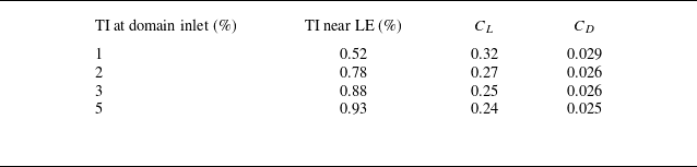
As reported in the literature (Michna & Rogowski Reference Michna and Rogowski2022), the aerodynamic forces are highly sensitive to turbulent intensity (TI). Therefore, to quantify how the forces change, a TI sensitivity study was performed. Here, the TI at the domain inlet was prescribed as 1 %, 2 %, 3 % and 5 %. Due to the decay of the turbulence intensity from the inlet to the leading edge (LE) of the wing, the turbulence intensity at the LE was much lower than those prescribed at the inlet. For the above inlet turbulence intensities, the associated lift and drag coefficients for
 $\alpha =2^\circ$
are tabulated in table 2. The study showed that both the lift and drag coefficients decreased when the TI was increased. As the LE TI increased from 0.52 % to 0.93 %, there was a 25 % and 14 % decrease in lift and drag, respectively, showing that lift is more sensitive to TI than drag in this case. For the rest of this study, CFD results are shown for an inlet TI of 5 %, as its associated TI at the LE was 0.9 %, which was close to the experimental conditions in the water tunnel.
Sensitivity of aerodynamic coefficients to TI for
 $\alpha =2^\circ$
(from 3-D CFD).

Table 2. Long description
A table with four rows and four columns. The columns are labeled ‘TI at domain inlet (%)’, ‘TI near LE (%)’, ‘C_L’, and ‘C_D’. The rows present the following data: Row 1: TI at domain inlet, 1 percent; TI near LE, 0.52 percent; C_L, 0.32; C_D, 0.029. Row 2: TI at domain inlet, 2 percent; TI near LE, 0.78 percent; C_L, 0.27; C_D, 0.026. Row 3: TI at domain inlet, 3 percent; TI near LE, 0.88 percent; C_L, 0.25; C_D, 0.026. Row 4: TI at domain inlet, 5 percent; TI near LE, 0.93 percent; C_L, 0.24; C_D, 0.025.
Two-dimensional CFD grid convergence study. (a) Lift convergence, (b) drag convergence and (c) pressure convergence at
 $\alpha = 2^\circ$
.

To validate the 3-D CFD solution, the lift and drag predictions, which were found by integrating pressure and shear stress over the entire surface of the wing, are compared with the experimental measurements in figures 7(a) and 7(b), respectively. The CFD predictions are shown for AoA increments of
 $\Delta \alpha =1^\circ$
. Figure 7(a) shows excellent agreement between CFD and experimental values of the lift coefficient (
 $C_L$
) and mutually captures a nonlinear variation with AoA. Relatively good agreement between the two techniques was found in the case of drag coefficient (
 $C_D$
) shown in figure 7(b), especially at moderate AoAs. The drag around
 $\alpha = 0^\circ$
is under-predicted by CFD. At low AoAs, the profile drag (skin friction and pressure drag) is dominating while the induced drag is minimal. Since drag is an order of magnitude lower than lift, it is particularly sensitive to surface roughness or other slight imperfections in the model that are not accounted for in the CFD analysis. This could be producing an extra profile drag contribution. In contrast, for higher AoAs where the induced drag dominates, there is better agreement between experiments and CFD.
Force comparison between 3-D CFD and measurements for Re = 50 000. (a) Lift coefficient (
 $C_L$
) and (b) drag coefficient (
 $C_D$
) varying with AoA.

3.1.2. Experiment accuracy
The 2-D PIV technique was applied to measure the streamwise (
 $U$
) and wall-normal (
 $V$
) velocity components. The laser plane was located at the spanwise position of
 $z/b$
= 0.6 to prevent the tip vortex (highly three-dimensional) from influencing the flow field. The previously validated CFD simulation assisted in the spanwise location selection. Figure 8 shows the spanwise velocity distribution (front view) predicted using CFD. The spanwise velocity (out-of-plane
 $w$
component) magnitude less than 1 % was assumed to be free of tip vortex influence, which was found inboard of
 $z/b$
= 0.6.
Wing front view showing normalised spanwise velocity distribution for
 $\alpha = 6^\circ$
(from CFD).

As the study requires an investigation into the behaviour of the boundary layer to characterise the flow, accurate and high resolution experimental measurements are required. The near-wall velocity vectors measured using micro-PIV are shown in figure 9(a), which shows a resolution of ∼18 vectors within the boundary layer. Furthermore, figure 9(b) shows a measured turbulent boundary layer in terms of viscous units,
 $U^+={u}/{u^*}$
(streamwise velocity) and
 $Y^+=yu^*/{\nu }$
(distance from the wall) at a chordwise location of
 $x/c =0.8$
, which is further downstream of the LSB, for
 $\alpha = 6^\circ$
. The friction velocity
 $u^*$
was obtained using the Clauser-chart method (Clauser Reference Clauser1956). To ensure the accuracy of the micro-PIV technique, the measured streamwise velocity was plotted against the theoretical viscous sublayer (
 $U^+ = Y^+$
) and log law of the wall (
 $U^+ = ({1}/{\kappa })ln(Y^+) + B$
) using
 $\kappa = 0.41$
and B = 5.5. The velocity measurements were resolved until
 $Y^+\approx 2$
and showed good agreement with the theoretical viscous sublayer but slightly deviated in the log law of the wall regions.
Micro-PIV measurements of boundary layer profiles. (a) Boundary layer profile for
 $\alpha = 4^\circ$
showing the vector resolution, (b) regions of a turbulent boundary layer captured for
 $\alpha = 6^\circ$
at
 $x/c = 0.8$
.

The force and velocity measurements were conducted at AoAs
 $\alpha = 0-12^\circ$
in
 $\Delta \alpha =2^\circ$
increments. Force measurements were performed using a 6-axis ATI load cell at a frequency of 1 KHz for each test case. Considering the fact that the present study investigates flow over an airfoil with LSBs, a data distribution analysis was performed to ensure that there was no bi-modality in the data that can skew the experimental observation (Jacob et al. Reference Jacob, Stewart, Benedict and Ramasamy2026).
3.2. Characterisation of LSB
A nonlinear trend was observed in the lift curve from both the computational analysis and the experiments (figure 7
a). Specifically, the lift curve can be decomposed into two distinct linear regions – a trend also found for a NACA 0018 airfoil from a study performed by Michna & Rogowski (Reference Michna and Rogowski2022). At low AoAs, the slope is slightly greater than
 $2\pi$
– the result from thin airfoil theory. For
 $\alpha \gt 4^\circ$
, the lift curve slope changes dramatically and becomes lower. To investigate this phenomenon, the flow field over the wing was examined. Figure 10 shows the boundary layer development over the upper surface for
 $\alpha = 6^\circ$
obtained using micro-PIV. The flow develops as laminar, then undergoes separation and reattaches as a turbulent boundary layer.
Measured boundary layer profiles using micro-PIV showing the formation of LSB including laminar separation and turbulent reattachment for
 $\alpha = 6^\circ$
.

The region between laminar separation and turbulent reattachment is defined as a LSB (O’Meara & Mueller Reference O’Meara and Mueller1987). The boundary layer profile was plotted at chordwise locations before separation and after reattachment as shown in figure 11. The streamwise velocity and wall-normal distance were normalised by the edge velocity (
 $U_e$
) and boundary layer thickness (
 $\delta$
), respectively. The streamwise velocity grows faster with the wall-normal distance after reattachment compared with before separation, indicating that the boundary layer profile has transitioned from laminar to turbulent. This turbulent boundary layer profile is also plotted in viscous units in figure 9(b).
Laminar (before separation) and turbulent (after reattachment) boundary layer profiles (from PIV for
 $\alpha =6^\circ$
).

Flow fields and the corresponding turbulent kinetic energy fields showing region of transition for
 $\alpha = 6^\circ$
. Flow field showing LSB from (a) PIV and (b) 3-D CFD. Turbulent kinetic energy fields from (c) PIV and (d) 3-D CFD.

A turbulent boundary layer is characterised by increasing fluctuations in velocity compared with a laminar boundary layer. The turbulent kinetic energy (TKE), given by
 $k =({1}/{2})(\overline {u'^2} + \overline {v'^2} + \overline {w'^2})$
, is used to quantify turbulence. Here,
 $\overline {u'}$
,
 $\overline {v'}$
and
 $\overline {w'}$
indicate the root-mean-squares of the streamwise, wall-normal and spanwise velocity components, respectively. Figure 12 shows the flow fields from PIV (left) and CFD (right) for
 $\alpha = 6^\circ$
. Figures 12(a) and 12(b) show the presence of an LSB while figures 12(c) and 12(d) show the corresponding TKE fields. There is a large increase in the TKE after an x/c location of 0.45 for CFD and 0.4 for PIV, indicating a region of transition.
To examine how the LSB changes with AoA, flow fields over the suction surface for
 $\alpha = 0^\circ {-}12^\circ$
are shown in figure 13. There is excellent agreement between PIV (a) and CFD (b) where the LSB can be seen moving towards the LE with increasing AoA.
Experimental (a) and 3-D CFD (b) flow fields of the suction side for varying AoAs (
 $\alpha$
). Arrows denote the movement of the LSB with AoA.

Figure 13. Long description
Panel A: Experimental flow fields. Panel B: 3-D CFD flow fields. Each panel contains multiple contour plots showing streamwise velocity on the suction side of an airfoil at different angles of attack (alpha). The x-axis represents the chordwise position (x/c) ranging from 0 to 1. The y-axis represents the spanwise position (y/c) ranging from −0.2 to 0.2. The color scale indicates streamwise velocity (U/U_infinity) with values ranging from −0.20 to 1.50. Arrows denote the movement of the laminar separation bubble (LSB) with increasing angle of attack.
Park et al. (Reference Park, Shim and Lee2020) and Toppings et al. (Reference Toppings, Kurelek and Yarusevych2021) also observed bubble movement toward the LE with an increasing AoA. The bubble can also be seen to be decreasing in length as it moves towards the LE. The separation and reattachment locations (representing the length of the LSB) are quantified in figure 14(a), which shows good agreement between PIV and CFD. These were identified by selecting the location where the wall shear stress goes to zero (
 $\tau _w=0$
). The bubble height is shown in figure 14(b) as a fraction of the airfoil thickness (15 % chord). Although the length can be seen decreasing in size, height remains fairly constant with AoA.
Laminar separation bubble size characterisation from PIV and 3-D CFD. (a) Separation and reattachment locations as fraction of chord showing the LSB’s movement towards the LE and decrease in length with increasing AoA, (b) LSB height in per cent thickness from PIV and 3-D CFD.

Next, to relate the presence of the LSB to changes observed in the lift curve, the pressure distribution around the wing needs to be examined. All pressure distributions shown in this paper were obtained from CFD. Because there is excellent agreement between the 3-D CFD and test data for the force and flow field measurements, the pressure obtained from CFD can be used with confidence. Figure 15 shows the chordwise pressure distribution along the suction surface for AoAs
 $4^\circ$
,
 $8^\circ$
and
 $12^\circ$
. The separation and reattachment locations are marked showing where the bubble is located. The pressure curve plateaus in the presence of the bubble.
Pressure distributions on the suction side for
 $\alpha = 4^\circ , 8^\circ , 12^\circ$
. The LSB location is marked by separation and reattachment points (from 3-D CFD).

To isolate the effect of the LSB on the pressure distribution and, in turn, the lift curve, a fully turbulent CFD analysis was performed using the
 $k-\omega $
SST model. The laminar-to-turbulent boundary layer transition was not taken into account, thus eliminating the formation of the LSB. Figure 16 shows the lift force and the corresponding pressure curves comparing the fully turbulent analysis (no LSB) with the laminar-to-turbulent transition analysis (with LSB) for
 $\alpha = 8^\circ$
. Figure 16(b) shows that the pressure curve is altered by the presence of the LSB. Also, in the absence of the LSB, i.e. fully turbulent model, the lift curve is linear, as shown in figure 16(a).
Transition model and fully turbulent model comparison for (a) lift coefficient, and (b) pressure coefficient for
 $\alpha = 8^\circ$
from 3-D CFD.

Velocity contours showing lower surface LSB and variation with
 $\alpha$
(3-D CFD); (a)
 $\alpha = 0^\circ$
, (b)
 $\alpha = 2^\circ$
, (c)
 $\alpha = 4^\circ$
, (d)
 $\alpha = 6^\circ$
, (e)
 $\alpha = 8^\circ$
.

Figure 17. Long description
Panel A: A contour plot showing streamwise velocity distribution with axes labeled x over c and y over c for angle of attack of 0 degrees. The color scale ranges from −0.20 to 1.50, indicating velocity values. The upper and lower surface laminar separation bubbles (LSB) are visible. Panel B: A contour plot showing the movement of the upper LSB towards the leading edge (LE) and the lower LSB towards the trailing edge (TE) for an angle of attack of 2 degrees. Panel C: A contour plot showing the upper LSB moving towards the LE and the lower LSB decreasing in size for an angle of attack of 4 degrees. Panel D: A contour plot showing the upper LSB moving further inboard and the lower LSB becoming negligible in size for an angle of attack of 6 degrees. Panel E: A heat map showing the upper LSB out of frame and the lower LSB no longer present for an angle of attack of 8 degrees.
The prior results in figures 12, 13, 14 and 15 highlighted the characteristics of the upper surface of the wing; however, attention should also be drawn to the lower surface. Figure 17 shows streamwise velocity contours over the lower surface of the wing, which evidently displays the existence of a lower surface LSB that has not been studied extensively in the previous literature. As the AoA increases, the lower surface separation point moves towards the trailing edge as the adverse pressure gradient decreases. The size of the bubble decreases with increasing AoA. At an AoA of
 $\alpha = 6^\circ$
, the lower LSB has almost vanished, and for
 $\alpha = 8^\circ$
, the lower bubble has completely vanished while the upper LSB is still present. The impact of the lower surface LSB on the overall pressure distribution will be discussed in a subsequent section.
3.3. Laminar separation bubble acts as a geometric feature
After the examination of the pressure curves and the surrounding flow fields of the LSB from both PIV and CFD, it is hypothesised that the presence of an LSB results in a virtual shape change (or virtual camber) of the airfoil. In other words, the LSB acts as if it were a geometric feature that alters the outer inviscid flow. To prove this hypothesis, several analyses were performed where the airfoil geometry was modified to account for the presence of the LSB. To simplify the analysis, the CFD was moved from three-dimensional to two-dimensional. Figure 18 compares the lift curve between the 2-D and 3-D analyses and verifies that the same nonlinear trend is observed for the 2-D case. This confirms that the nonlinearity in lift is not a 3-D effect. The 2-D analysis shows a higher lift coefficient and lift slope, which are both characteristic of infinite AR versus finite AR wings that produce tip vortex induced downwash. With this 2-D analysis, the methods to prove the hypothesis are discussed in detail below.
Comparison of lift coefficient versus AoA for 2-D and 3-D CFD.

3.3.1. Inviscid method
The first method investigates the effect of the LSB on the outer flow using an inviscid analysis. This method began by finding the displacement thickness of the original NACA 0015 airfoil (CFD analysis that considers the laminar-to-turbulent transition), denoted by
 $\delta _0^*$
. The airfoil was then modified with
 $\delta _0^*$
, and an inviscid analysis was run for the modified profile.
The displacement thickness was found using (3.1) where
 $U(y)$
is the wall-normal velocity profile. The boundary layer thickness,
 $\delta$
, as well as the local edge velocity,
 $U_e$
, were identified using the local reconstruction method (LRM) by Griffin et al. (Reference Griffin, Fu and Moin2021)
 \begin{equation} \delta ^*=\int _0^\infty \left ( 1-\frac {U(y)}{U_e}\right)\text{d}y. \end{equation}
The LRM at
 $\alpha =2^\circ$
for chordwise stations: (a) x/c = 0.41 (before separation), (b) x/c = 0.71 (separated region), (c) x/c = 0.95 (after reattachment).

Figure 19. Long description
Panel A: A line graph shows the viscous and inviscid profiles at the chordwise station x/c = 0.41. The y-axis represents the normalized height y/δ, and the x-axis represents the normalized velocity U/UE. The viscous profile is depicted by a solid blue line, while the inviscid profile is shown by a dashed orange line. A red dot marks the position δ99. Panel B: A line graph illustrates the viscous and inviscid profiles at the chordwise station x/c = 0.71. The axes and line styles are the same as in Panel A, with a red dot indicating the position δ99. Panel C: A line graph presents the viscous and inviscid profiles at the chordwise station x/c = 0.95. The axes and line styles are consistent with the previous panels, and a red dot marks the position δ99.
The LRM presents an accurate and computationally inexpensive way to determine the boundary layer thickness which does not rely on empirical data like other methods. In essence, the basis of the LRM is that (i) viscous effects are confined to be within the boundary layer,
 $y \lt \delta$
, and (ii) the flow is approximately inviscid and irrotational for
 $y\gt \delta$
. Under these assumptions, the Bernoulli equation can be applied globally rather than just along a streamline; thus, a reconstructed inviscid velocity, denoted by
 $U_I$
, can be defined by (3.2) where
 $y$
is the wall-normal coordinate,
 $P_{o,\textit{ref}}$
, is the reference stagnation pressure,
 $P(y)$
is the static pressure and
 $V(y)$
is the wall-normal velocity
 \begin{equation} U_I=\sqrt {\frac {2}{\rho }[P_{o,\textit{ref}} - P(y)] - V^2(y)}. \end{equation}
For different chordwise stations, the local reconstructed velocity profile (inviscid profile) is compared with the original velocity profile (viscous profile) and is shown in figure 19. The boundary layer is defined as the region near the wall where the viscous profile disagrees with the inviscid profile. Outside of the boundary layer, the inviscid profile is almost identical to the viscous profile. The boundary layer thickness is labelled for each chordwise location according to the definition in (3.3). The edge velocity was then taken to be
 $U_e=U(y=\delta _{99})$
 \begin{equation} \left . \frac {U(y)}{U_I} \right |_{y=\delta }=\frac {99}{100}. \end{equation}
The displacement thickness was computed for both the suction and the pressure side of the NACA 0015 airfoil. The airfoil geometry was then modified using the displacement thickness. This modified geometry is shown in figure 20(a). Finally, an inviscid simulation using XFOIL (Drela Reference Drela1989) was run for the modified geometry.
The pressure distribution from the inviscid simulation is plotted in figure 20(b), and is compared with that of the original airfoil. There is good agreement between the two, as the inviscid analysis was able to capture the plateaus in pressure caused by the presence of the upper and lower LSBs. The root mean square error (RMSE) between the two
 $C_{\!p}$
curves was 0.046. Furthermore, the absolute difference between the original and inviscid lift coefficients was 0.010. This agreement proves that the LSB effectively thickened the airfoil as seen by the outer flow.
(a) Geometry comparison between the NACA 0015 profiles: original and modified with
 $\delta _0^*$
, (b) comparison of pressure distributions between the original profile and the modified profile with
 $\delta _0^*$
(inviscid analysis) for
 $\alpha = 2^\circ$
.

3.3.2. Displacement thickness subtraction method
While the inviscid analysis showed the overall effect of the LSB on the pressure curve, the geometry of the LSB was not directly used in the analysis. In order to claim that the LSB acts as a geometric feature, the LSB profile was extracted using fundamental principles and added to the original airfoil. With this modified airfoil, a fully turbulent CFD analysis was run to suppress the formation of additional LSBs. Finally, the pressure distribution of the original airfoil was compared with that of the modified airfoil.
Similar to the inviscid analysis, this method begins by finding the displacement thickness of the original airfoil,
 $\delta _0^*$
. However, in order to isolate the LSB geometry, the displacement thickness caused by (i) the boundary layer and (ii) the free shear layer profile that formed over the LSB (viscous region between the dividing streamline and the outer flow (Horton Reference Horton1968)) needs to be subtracted. One approach is to find the
 $\delta ^*$
of the original airfoil with the LSB suppressed and then subtract it from
 $\delta _0^*$
. This means that a fully turbulent boundary layer will form over the original airfoil. The problem with this approach is that in the locus of the LSB, the
 $\delta ^*$
from the fully turbulent boundary layer is not representative of the
 $\delta ^*$
caused by the free shear layer above the curvature of the LSB. To rectify this, a fully turbulent simulation was run on the airfoil modified with
 $\delta _0^*$
and the displacement thickness of this modified airfoil,
 $\delta _{mod}^*$
, was computed. This choice of displacement thickness approximately takes into account the influence of the LSB curvature on the shear layer profile. Finally,
 $\delta _{mod}^*$
was subtracted from
 $\delta _0^*$
, resulting in the isolated LSB geometry given by
 $\varDelta =\delta _0^*-\delta _{mod}^*$
.
(a) Geometry comparison between the NACA 0015 profiles: the original profile (blue curve) and the modified profile with LSBs incorporated as a geometry (red curve). In this case, the LSB geometry was obtained using the displacement thickness subtraction method (DTSM). (b) Comparison of pressure distributions between the original profile and the modified profile for
 $\alpha = 2^\circ$
.

The LSB geometry
 $\varDelta$
, was then added to the original airfoil profile (denoted DTSM airfoil) as seen in figure 21(a), and a fully turbulent analysis was run. Figure 21(b) compares the pressure distributions of the DTSM airfoil and the original airfoil. There is excellent agreement between them proving the hypothesis that the LSB can be treated as a geometric feature in regard to pressure. The RMSE between the two
 $C_{\!p}$
curves was 0.018. Furthermore, the absolute difference between the corresponding lift coefficients was 0.026.
Despite the agreement, the validity of the fully turbulent boundary layer assumption needs to be assessed; particularly, the approximation of the free shear layer above the LSB as a turbulent boundary layer. To this end, an inviscid analysis was performed to confirm that the total displacement seen by the outer flow from this approximation is the same as the original displacement thickness,
 $\delta _0^*$
. First, the displacement thickness was computed for the DTSM airfoil and then added to the DTSM profile. Then an inviscid analysis was run for the modified geometry (Inviscid DTSM) shown in figure 22(a). Compared with the original airfoil modified with
 $\delta _0^*$
(Inviscid method), there is great agreement between the two geometries. Furthermore, figure 22(b) compares the pressure distribution from this analysis and the inviscid method from the previous section (figure20
b). Here, the RMSE was calculated to be 0.0178.
There is great agreement between the two methods – both geometry and pressure – proving that the fully turbulent boundary layer forming over the bubble geometry is a good approximation. In other words, the total displacement of the outer inviscid flow can be separated into a contribution from the LSB geometry as well as an additional thickness from the free shear layer that can be treated as a boundary layer forming over the LSB.
(a) Geometry comparison between the original NACA 0015 profile modified with its displacement thickness,
 $\delta _0^*$
, and the DTSM profile (original airfoil with LSB incorporated as geometry) modified with its displacement thickness, (b) comparison of the pressure distributions obtained for the two geometries for
 $\alpha = 2^\circ$
(inviscid analysis).

3.3.3. Dividing streamline method
The final method takes a more direct approach in extracting the LSB profile using its dividing streamline and adding it to the original airfoil. With this modified airfoil, a fully turbulent CFD analysis was run to suppress the formation of additional LSBs. Finally, the pressure distribution of the original airfoil is compared with that of the modified airfoil where the LSBs are part of the airfoil’s geometry.
The detailed process of creating the modified airfoil geometry that includes the shape of the LSB is described in figure 23. First, a 2-D CFD analysis was performed for the unmodified NACA 0015 airfoil considering the laminar-to-turbulent transition. Using the flow fields generated from this analysis, such as in figure 23(a), the LSBs were identified using their dividing streamlines (figure 23 b). This is defined as the streamline that passes through both the laminar separation point and the turbulent reattachment point (Horton Reference Horton1968). With knowledge of the X and Y points that correspond to the dividing streamline, the bubble shape was incorporated into the airfoil surface as shown in figure 23(c) and is compared with the original airfoil geometry in figure 24(a).
Process of creating the modified airfoil profile. (a) Flow field showing the LSBs, (b) isolating and extracting the LSB geometry, (c) modified airfoil profile where the LSB is incorporated as geometry.

Figure 24(b) compares the pressure distribution between the original airfoil and the modified airfoil for
 $\alpha =2^\circ$
where the RMSE was 0.016 and the absolute difference in lift coefficient was 0.0033. Similar to the DTSM, there is also good agreement with the original pressure distribution. In fact, the LSB profile obtained from the DTSM matched almost identically with the dividing streamline as shown in figure 25. This reinforces the claim that the LSB geometry, defined by their dividing streamline, can be treated as a solid addition to the airfoil profile. In addition to the pressure distribution, the velocity fields that compare the original airfoil with the modified airfoil at
 $\alpha = 2^\circ$
are shown in figure 26. The modified flow field largely resembles the original flow field, providing further evidence for this argument.
(a) Geometry comparison between the NACA 0015 profiles: the original profile (blue curve) and the modified profile with LSBs incorporated as a geometry (red curve). In this case, the dividing streamline was taken as the LSB geometry. (b) Comparison of pressure distributions between the original profile and the modified profile for
 $\alpha = 2^\circ$
.

Comparison of the NACA 0015 airfoil profiles that were modified by the LSB geometry obtained from (i) the dividing streamline method (blue curve) and (ii) the DTSM (red curve) showing great agreement.

Flow field comparison between (a) original and (b) modified airfoil with upper and lower LSBs for
 $\alpha = 2^\circ$
.

3.4. Isolated effects of LSBs
As mentioned previously, most studies in the literature focus on the suction side LSB. However, the NACA 0015 airfoil has an LSB on both the suction and pressure sides at a Reynolds number of 50 000. This section focuses on isolating the effects of the upper and lower LSBs on the overall pressure distribution. For the remainder of this paper, the dividing streamline method will be used due to its simplicity and the ease with which it can isolate the bubble geometry.
Using this method, the upper and lower LSBs were extracted and then separately analysed for
 $\alpha =2^\circ , 4^\circ , 6^\circ , 8^\circ$
. The analysis featured three subcases in which the original airfoil was modified with: (i) only the upper LSB, (ii) only the lower LSB and (iii) with both the upper and the lower LSBs. For each of these modified airfoils, a fully turbulent analysis was run.
Isolated effects of upper and lower LSBs on the pressure distribution for
 $\alpha = 2^\circ$
. Comparison of the modified airfoils with (a) original NACA0015 airfoil with LSB formation suppressed (simulation without transition model), (b) original NACA0015 airfoil (simulation with transition model allowing natural LSB formation).

The results of the subcases are presented in figure 27, which shows the surface pressure distributions over the modified geometry for the case of
 $\alpha =2^\circ$
. Figure 27(a) begins by comparing the pressure distributions of the modified upper and lower airfoils with that of the original airfoil with the LSBs numerically suppressed (fully turbulent analysis). Compared with the original airfoil with no LSBs, the addition of the upper surface LSB to the airfoil geometry resulted in a local change in pressure to only the upper surface between
 $x/c \approx 0.3$
and
 $x/c \approx 0.8$
. Otherwise, the pressure distribution matches well with the unmodified airfoil. This heavily contrasts to the case where only the lower surface LSB was added to the geometry, as the pressure distribution was altered for the whole chord length and on both the upper and lower surfaces of the airfoil.
Figure 27(b) compares the pressure distributions of the modified upper and lower airfoils with that of the original NACA0015 airfoil that considered laminar-to-turbulent transition. Firstly, the difference in pressure between the upper and lower surfaces is greater for the original airfoil than for the one modified with upper LSB for all
 $x/c$
locations. However, between
 $x/c \approx 0.5$
and
 $x/c \approx 0.8$
, the upper surface pressure plateaus and is followed by a sharp adverse pressure gradient that is almost identical to the original airfoil. Figure 27(b) also compares the original with the modified airfoil with the lower LSB, where the pressure distribution almost exactly matches except for the upper surface between
 $x/c \approx 0.5$
and
 $x/c \approx 0.8$
where the upper LSB is located. Notably, the lower LSB has caused an increase in pressure on the lower surface and a decrease in pressure on the upper surface.
Downward shift of chord line due to lower LSB which introduces both camber and an incidence angle.

Figure 27 shows that the inclusion of the lower surface LSB had a much greater impact on the pressure distribution than the upper LSB. This is because the lower LSB extended to the trailing edge which effectively rotated the chord line to a positive incidence – similar to the behaviour of a trailing edge flap – demonstrated by the schematic shown in figure 28. This had two effects: (i) the modified airfoil’s AoA has been increased relative to the oncoming flow, and (ii) the camber of the entire airfoil has been modified. These effects impact the behaviour of the entire airfoil, providing insight into why the entire pressure distribution changed when the lower surface bubble was included (figure 27). In contrast, for the airfoil modified with the upper LSB, the trailing edge remained unaltered, resulting in only a localised change in camber.
Now having examined the effects of the upper and lower LSBs separately, the next step is to examine their combined effects. Figure 29 compares the original airfoil pressure distribution with that of the (i) modified geometry with the upper LSB and the (ii) modified geometry with the upper and lower LSBs for
 $\alpha = 2^\circ$
,
 $\alpha = 4^\circ$
,
 $\alpha = 6^\circ$
and
 $\alpha = 8^\circ$
(figure 29(a–d), respectively). For all AoAs, the pressure distribution of the modified airfoil with both the upper and lower LSBs is almost identical to that of the original airfoil. While the inclusion of the lower LSB had a large effect on the pressure distribution for
 $\alpha =2^\circ$
, this diminishes quickly with increasing AoA as the lower bubble decreases in size (figure 17). At
 $\alpha = 6^\circ$
, the bubble size becomes negligible and by
 $\alpha =8^\circ$
, the lower LSB has completely vanished, which is reflected in figures 29(c) and 29(d).
Comparison of original airfoil pressure distribution with (i) modified airfoil with only the upper LSB and (ii) modified airfoil with both the upper and lower LSBs for (a)
 $\alpha = 2^\circ$
, (b)
 $\alpha = 4^\circ$
, (c)
 $\alpha = 6^\circ$
and (d)
 $\alpha = 8^\circ$
.

3.5. Correlation of LSB with nonlinear lift
Having examined the pressure distributions, the next step is to examine the integral quantities of the modified airfoils such as the lift coefficient and use the previously gained insights to explain the nonlinear behaviour in the lift curve. While lift produced by the airfoil depends on the AoA, there is a secondary variation in that the LSB geometry also changes in size and location as a function of AoA.
To separate these variations, figure 30(a) shows the AoA sweeps for each of the modified airfoils (modified with both the upper and lower LSBs) that were previously examined in figure 29(a–d). Here, the modified airfoil extracted from
 $\alpha = 2^\circ$
(
 $M-2^\circ$
, for short) has the highest lift, and the modified airfoil from
 $\alpha = 8^\circ$
(
 $M-8^\circ$
) has the lowest lift. Furthermore, in figure 30(a) the lift curves for the
 $M-2^\circ$
and
 $M-4^\circ$
airfoils are much higher than the lift curves for the
 $M-6^\circ$
and
 $M-8^\circ$
. The reason for the higher lift stems from the presence of the lower LSB that extends to the trailing edge (figure 28). This results in a global change in the camber distribution (figures 29
a and 29
b) as opposed to a non-trailing edge LSB that only results in a local change (figures 29
c and 29
d). As the AoA increases, the lower bubble decreases in size (shown in figure 17). The lower LSB is much larger for the
 $M-4^\circ$
airfoil than for the
 $M-6^\circ$
, resulting in a notable upward shift in the lift curve.
Figure 30(a) also demonstrates the combined effect of AoA and LSB variations. As each airfoil was modified using an LSB formed at a specific angle, the lift extracted for only that angle is denoted by black points. The red dashed line connects these extracted lift values from the different modified airfoils and captures the combined effect of AoA and geometry change. From
 $\alpha =0^\circ$
to
 $\alpha = 2^\circ$
, there is a large increase in virtual camber, which causes the change in lift to be very large (greater than
 $2\pi$
). From
 $\alpha = 2^\circ$
and further, the virtual camber begins to decrease. Notably, a sharp decrease in lift is observed for
 $\alpha = 4^\circ$
to
 $\alpha = 6^\circ$
as the size of the lower LSB becomes negligible.
Figure 30(b) summarises the effort by comparing the predicted lift for the modified airfoils (black points from figure 30(a)) with that of the original NACA 0015 (blue curve). The modified geometry for all AoAs shows good agreement with the original airfoil, confirming that the LSB, whether on the upper or lower surface, acts as a geometric feature. Furthermore, this demonstrates that the nonlinear behaviour of the lift curve is primarily due to the varying presence of the lower and upper LSBs. To elaborate, the lift curve of the original airfoil can be broken into two distinct regions, one where the lower bubble is present, and one without. The lower bubble size is significant between
 $\alpha =0^\circ$
and
 $\alpha = 4^\circ$
, resulting in a higher camber and incidence angle (figure28) that shifts the lift curve upward. From angles greater than
 $\alpha = 4^\circ$
, the size becomes negligible and the bubble eventually vanishes after
 $\alpha = 6^\circ$
, which greatly reduces the camber. Comparing the regions of the lift curve where the lower surface LSB is present with those regions without the lower bubble, there is a significant increase in the lift slope in the regions that have a lower LSB.
Combined effect of increasing AoA and changing geometry. (a) Lift curves for the modified airfoils, (b) comparison between original airfoil lift curve and the lift extracted from the modified airfoils (black points from (a).

Figure 30. Long description
Panel A: A line graph shows lift coefficient (C_l) on the vertical axis and angle of attack (degrees) on the horizontal axis. Multiple lines represent different modified airfoils: blue for airfoil modified with 2 degrees upper and lower LSB, orange for 4 degrees upper and lower LSB, yellow for 6 degrees upper and lower LSB, and purple for 8 degrees upper LSB. A red dashed line indicates the combined effect of increasing angle of attack and changing geometry. Panel B: Another line graph compares the lift coefficient of the original airfoil (blue line) with the lift extracted from the modified airfoils (black points from Panel A). The horizontal axis is angle of attack (degrees), and the vertical axis is lift coefficient (C_l).
4. Summary and conclusions
A combined experimental and computational analysis was carried out to characterise airfoil behaviour at low Reynolds number (50 000). Experiments were conducted in a water tunnel to obtain lift and drag measurements. Micro-PIV was performed to resolve the velocity profile in the boundary layer. The computational results were validated with the experimental data. Following validation, the CFD results were used to analyse and explain the observations made in the experiments. Substantial effort was made to ensure that the measurements are reliable and that computational predictions follow state-of-the-art procedures. In the case of experiment, statistical analysis was carried out; for CFD, the uncertainty analysis included the estimation of errors from modelling, grid resolution and iteration. The following are the specific conclusions derived from the study.
-
(i) Computational fluid dynamics using the RANS equations with the
 $k-\omega $
SST turbulence model and
$\gamma -\textit{Re}_\theta$
transition model exhibited strong agreement with experimentally measured loads, velocity fields and the size and location of LSBs. Excellent correlation was found between experiment and CFD in the case of measured lift. In the case of drag, CFD under predicted the values at low AoA but showed an excellent correlation otherwise. Streamwise velocity contours at
$z/b = 0.6$
of the wingspan matched almost identically between CFD and high fidelity micro-PIV measurements.
-
(ii) Laminar separation bubbles, defined by their dividing streamline, can be treated as a geometric feature that alters the outer inviscid flow. The LSB profile obtained using fundamental principles (DTSM) was almost identical to its dividing streamline, proving that it can be treated as a solid addition to the airfoil geometry. After extracting the shape of the LSBs and including them as part of the geometry of the NACA 0015 airfoil, the surface pressure distribution of this modified airfoil matched almost identically with that of the original airfoil for varying AoAs.
-
(iii) The lower surface LSB that extends to the trailing edge is the primary source of lift augmentation, and its vanishing produced a distinct two-slope lift curve. The CFD analysis revealed an LSB on the lower surface that vanishes after
$\alpha = 6^\circ$
. By modelling the LSB as a geometric feature, the study revealed that the lower surface LSB provides a large increase in virtual camber and is the primary source of lift augmentation.


Acknowledgements
The authors acknowledge Texas A&M High Performance Research Computing (HPRC) for providing computational resources to perform the CFD analysis. The authors also express their gratitude to the peer reviewers whose valuable feedback helped enhance this study.
Funding
This work was jointly supported by the Vertical Lift Research Center of Excellence (VLRCOE) under Award Number W911W6-21-2-0003—led by the University of Maryland and sponsored by the U.S. Army, U.S. Navy, and NASA—and by the U.S. Army Research Laboratory under Cooperative Agreement Number W911NF-21-2-0188. The views and conclusions contained in this document are those of the authors and should not be interpreted as representing the official policies, either expressed or implied, of the Army, NASA, or the U.S. Government. The U.S. Government is authorised to reproduce and distribute reprints for Government purposes, notwithstanding any copyright notation herein.
Declaration of interests
The authors declare none.
Author contributions
S.J. performed the experiments and R.-W.S. performed the simulations. All authors contributed equally to analysing data, reaching conclusions and in writing the paper.


 α
 ∘

 α=2∘

 α=2∘

 α=2∘

 CL
 CD

 α=6∘

 α=4∘
 α=6∘
 x/c=0.8

 α=6∘

 α=6∘

 α=6∘

 α


 α=4∘,8∘,12∘

 α=8∘

 α
 α=0∘
 α=2∘
 α=4∘
 α=6∘
 α=8∘


 α=2∘

 δ0∗
 δ0∗
 α=2∘

 α=2∘

 δ0∗
 α=2∘


 α=2∘


 α=2∘

 α=2∘


 α=2∘
 α=4∘
 α=6∘
 α=8∘


 Open access

