


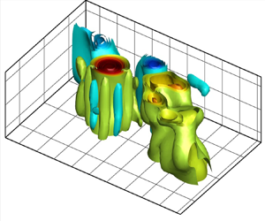



1. Introduction
The understanding of fluid–structure–surface interactions in submerged hydrodynamic bodies is crucial for a wide variety of applications, such as near-surface energy harvesters, floating wind farms, marine structures and tidal power generation equipment. Flow-induced vibration (FIV) of these systems can be significantly affected by asymmetry, which can be either geometric or flow-dependent. Despite extensive studies on geometric asymmetry, such as the asymmetric boundary condition of the structure (Bourguet & Jacono Reference Bourguet and Jacono2014; Seyed-Aghazadeh, Edraki & Modarres-Sadeghi Reference Seyed-Aghazadeh, Edraki and Modarres-Sadeghi2019; Bourguet Reference Bourguet2021), cross-section (Nemes et al. Reference Nemes, Zhao, Jacono and Sheridan2012; Seyed-Aghazadeh, Carlson & Modarres-Sadeghi Reference Seyed-Aghazadeh, Carlson and Modarres-Sadeghi2017; Chen et al. Reference Chen, Ji, Alam, Xu, An, Tong and Zhao2022) and various angles of attack (Seyed-Aghazadeh, Budz & Modarres-Sadeghi Reference Seyed-Aghazadeh, Budz and Modarres-Sadeghi2015; Bourguet & Triantafyllou Reference Bourguet and Triantafyllou2016; Seyed-Aghazadeh & Modarres-Sadeghi Reference Seyed-Aghazadeh and Modarres-Sadeghi2018; Seyed-Aghazadeh et al. Reference Seyed-Aghazadeh, Benner, Gjokollari and Modarres-Sadeghi2021), the influence of flow asymmetry has not been as thoroughly investigated. Numerical studies have investigated the influence of shear flow in the cross-flow direction, characterised by a non-uniform velocity profile, on the fluid–structure interaction response of circular cylinders (Singh & Chatterjee Reference Singh and Chatterjee2014; Tu et al. Reference Tu, Zhou, Bao, Fang, Zhang, Li and Han2014; Zhang et al. Reference Zhang, Fan, Chen, Li and Li2014; Gsell, Bourguet & Braza Reference Gsell, Bourguet and Braza2017). These studies have revealed significant effects on the dynamic behaviour and the resultant fluid and structural forces in the presence of shear flow. The complexity of the effect of shear and associated symmetry breaking on FIV becomes apparent as the response depends on the direction and magnitude of the shear. For instance, Gsell et al. (Reference Gsell, Bourguet and Braza2017) identified three distinct regimes and found that shear plays a significant role in reshaping the wake pattern. This includes the development of an asymmetric pattern and changes in vortex shedding frequencies. Furthermore, shear flow can affect the synchronisation between vortex shedding and structural oscillation, which is a key factor in determining the oscillation amplitude. Depending on the sign and magnitude of the shear, the synchronisation region may shift, widen or narrow, leading to different FIV regimes and responses. In this study, we focus on the role of flow asymmetry on a self-excited oscillating flat plate with one and two degrees of freedom (DoFs). We introduce an asymmetric flow condition by reducing the distance between the flat plate and the water's free surface, thereby altering the gap ratio between the body and the free surface, denoted as  $H^*=H_o/t$ (where
 $H_o$ is the submerged height and
 $t$ is the thickness of the plate).
Vortex interaction with the water's free surface is a complex fluid dynamic phenomenon, leading to various physical effects such as surface deformation, wave creation, turbulence and mixing (Sarpkaya Reference Sarpkaya1996). The interaction can take complex forms depending on factors such as the vortex's size and strength and the fluid flow's velocity and direction. Vortex fragmentation is a common interaction between vortices and the free surface of water. Another form of vortex interaction with the water's free surface is the generation of surface waves. This can happen when a strong vortex collides with a free surface and the fluid flow within the vortex creates pressure differences that warp the surface. In particular, for large, powerful vortices, the resulting waves can be significant, leading to a considerable energy transfer from the fluid to the waves. In addition to fragmentation and wave development, a vortex's interaction with the water's free surface can result in other complicated phenomena, such as vortex pairing and merging and the formation of a coherent structure (surface vortices).
Numerous numerical and experimental studies have explored the relationship between the bluff bodies (such as cylinders or spheres) and the free surface, showing that as the submerged height of the structure decreases, the FIV response changes considerably (Sheridan, Lin & Rockwell Reference Sheridan, Lin and Rockwell1995; Saelim Reference Saelim1999; Reichl, Hourigan & Thompson Reference Reichl, Hourigan and Thompson2005; Chung Reference Chung2016; Sareen et al. Reference Sareen, Zhao, Sheridan, Hourigan and Thompson2018; Rajamuni, Hourigan & Thompson Reference Rajamuni, Hourigan and Thompson2021). These changes include a reduction in oscillation amplitude, alterations in the flow velocity over which large-amplitude oscillations are observed, known as the lock-in range, and a transformation of the symmetric wake into an asymmetric wake with irregular vortex generation. For instance, the work of Saelim (Reference Saelim1999) examined the 1DoF self-excited vortex-induced vibration (VIV) of a cylinder near the free surface in the range of  $H^*=0\unicode{x2013}3$. Their findings indicated a decrease in lock-in at
 $H^*=0.5$ compared with a deeply submerged case, while further reduction of
 $H^*<{0.5}$ expanded the VIV region to higher reduced velocities. A similar pattern was observed by Chung (Reference Chung2016) in their numerical study of a 2DoF cylinder undergoing VIV, where decreasing
 $H^*$ led to expanded lock-in ranges at higher reduced velocities and maximum oscillation amplitudes. The role of the Froude number (
 $Fr$), defined as
 $Fr=U_\infty /\sqrt {gH}$ (where
 $U_\infty$ is the flow speed,
 $g$ the gravitational acceleration and
 $H$ is the submerged height), and submerged height at constant Reynolds number
 $Re$ was explored by Reichl et al. (Reference Reichl, Hourigan and Thompson2005). Their results showed that at low values of
 $Fr=0$–
 $0.2$, when surface deformation was minimal, the wake exhibited similar characteristics to that of a submerged cylinder in an infinite medium, showing a symmetrical vorticity distribution around its centreline and the free surface interface could be assumed to be a free-slip wall. However, as the Froude number increased in the range of
 ${Fr=0.3\unicode{x2013}0.7}$, surface deformation effects became more pronounced, leading to irregular vortex generation. These findings align with the results of Sheridan et al. (Reference Sheridan, Lin and Rockwell1995) where they studied the wake vorticity pattern of circular cylinders close to the free surface at a large Reynolds number.
The majority of studies exploring the effect of free surface on streamlined structures have focused on the theoretical and computational examination of two-dimensional stability conditions. For example, within the potential flow framework, the linear interaction between a two-dimensional thin foil and a flat plate with the free surface has been studied both theoretically (Plotkin Reference Plotkin1975) and numerically (Giesing & Smith Reference Giesing and Smith1967; Yeung & Bouger Reference Yeung and Bouger1979). Moreover, the effect of the free surface via high-order perturbation theory has also been investigated (Salvesen Reference Salvesen1969; Kennell & Plotkin Reference Kennell and Plotkin1984). Tsai & Yue (Reference Tsai and Yue1993) investigated the fully nonlinear interaction between the free surface and body vortex, focusing on the dynamics of a near-surface vortex shedding from the base of a moving surface-piercing strut. They employed a fully nonlinear mixed Eulerian–Lagrangian approach, enabling them to explore the nonlinear interaction between the free surface wave and vortex bodies. The study's conclusion highlighted the dominant influence of the Froude number ( $Fr$) on the system dynamics. It revealed that for
 $Fr$ values exceeding one, a significant vortex–wave coupling is observed, whereas, for lower
 $Fr$ numbers, the interaction between the free surface wave and vortex structures is negligible. Investigating viscous effects in the context of steady transitional behaviours of a submerged foil, Chen & Chwang (Reference Chen and Chwang2002) implemented the finite-element method to compute Navier–Stokes equations. They found that the presence of a free surface amplifies the frequency of vortex shedding at specific Reynolds numbers. Meanwhile, Grue, Mo & Palm (Reference Grue, Mo and Palm1988) utilised a frequency-domain integral equation approach to study the flow around a two-dimensional flat plate at its free surface. Their work focused on energy harvesting from incoming waves using a thrust-generating foil and demonstrated the feasibility of extracting kinetic energy from free-surface waves. In a separate study, Cleaver et al. (Reference Cleaver, Calderon, Wang and Gursul2013) tested a NACA 0012 airfoil plunging near a free surface at various frequencies to investigate the influence of oscillation amplitude and submerged depth on drag reduction. They compared the measured forces with those obtained from a deeply submerged foil. Their findings highlighted that proximity to the free surface resulted in increased drag, whereas surface waves altered the flow field near the foil, leading to reduced thrust. A computational study by Zhu, Liu & Yue (Reference Zhu, Liu and Yue2006) explored horizontal and vertical three-dimensional NACA 0012 foil with forward motion near the free surface. Their results indicated a more pronounced effect of the free surface on the horizontal case compared with the vertical case. Specifically, in the horizontal case, the presence of the free surface significantly reduced both the mean thrust and propulsive efficiency of the foil. In contrast, the vertical foil exhibited a smoother variation in these parameters without such pronounced reductions. Moreover, free surface waves were primarily induced by oscillatory motion rather than the steady Kelvin waves resulting from the foil's forward motion (Sarpkaya Reference Sarpkaya1996).
Despite these extensive studies, there has been relatively little experimental focus on the visual quantification of three-dimensional asymmetric flow in self-excited oscillating plates or foils. This study seeks to bridge this gap by offering a qualitative and quantitative visualisation of three-dimensional asymmetric flow dynamics over a self-excited oscillating flat plate. In addition, we examine the structural dynamic response of the self-oscillating plate in close proximity to the free surface. This contribution enriches our comprehension of fluid–structure–surface interaction by providing detailed insights into the complex flow behaviour and its interaction with the plate's oscillation. The formation and subsequent shedding of a vortex from a streamlined structure undergoing unsteady pitching and plunging motions has consistently inspired scientists seeking to better understand swimming and flapping flight mechanisms (Wang Reference Wang2005; Lauder Reference Lauder2015). Numerous studies have investigated the stability, formation time, and circulation of the leading-edge vortex (LEV) and trailing-edge vortex (TEV) shedding dynamics in oscillating unbounded airfoils and plates (Gharib, Rambod & Shariff Reference Gharib, Rambod and Shariff1998; Ringuette, Milano & Gharib Reference Ringuette, Milano and Gharib2007; Taira & Colonius Reference Taira and Colonius2009; Wojcik & Buchholz Reference Wojcik and Buchholz2014; Eslam Panah, Akkala & Buchholz Reference Eslam Panah, Akkala and Buchholz2015; Onoue & Breuer Reference Onoue and Breuer2016; Zhu, Su & Breuer Reference Zhu, Su and Breuer2020).
Understanding the significance of LEV and TEV shedding in relation to the dynamic response of the oscillating streamlined structure is critical for the creation of physical models that can effectively control the system, particularly when significant disturbances such as free surface are present. As discussed previously, when a streamlined structure operates near the free surface, both the structure and the generated vortex wake can have a significant influence on the free surface of the water. In such an asymmetric flow condition, it is plausible that the dynamic behaviour of the structure and its LEV and TEV shedding pattern might deviate significantly from that of an unbounded fluid, and the wave patterns or imprints left on the free surface may possess their own distinct features. Despite this, the fundamental principles of the self-excited oscillating horizontal plate close to the free surface have received minimal experimental investigation. Therefore, this experimental investigation sheds light on the complex fluid–structure–surface interactions experienced by a flexibly mounted rigid flat plate undergoing free oscillations in both the pitching and plunging directions near a free surface. It emphasises the effect of reduced velocity, proximity to the free surface and vortex dynamics on the plate's FIV response. The reduced velocity is defined as  $U^*={U}/{f_{n1}C}$, where
 $U$ is the flow velocity,
 $C$ is the chord length of the plate and
 $f_{n1}$ is the pitching natural frequency of the system. The dynamic response of the plate, capable of oscillating in 1DoF and 2DoF systems, is explored for a range of reduced velocities of
 $U^*=0.29\unicode{x2013}8.73$, corresponding to a Reynolds number range of
 $Re=518\unicode{x2013}15{\,}331$.
The structure of this paper is as follows. Section 2 outlines the experimental set-up and methodology employed to measure the FIV response of the plate. The findings discussed in § 3 detail the overall FIV response of the plate over the complete range of tested flow velocities. Section 3.1 provides a description of oscillation amplitudes and frequency analysis, along with an exploration of response phase evolution across a wide range of flow velocities. Sections 3.2.1 and 3.2.2 present both qualitative and quantitative analysis of the wake structure at selected flow velocities. Lastly, § 3.2.3 offers a three-dimensional analysis of velocity vectors through the proper orthogonal decomposition (POD) method, with a specific focus on coherent structures such as LEV and TEV, as well as the interaction of vortices in the wake and at the free surface.
2. Experimental set-up and data collection
2.1. Structural response measurements
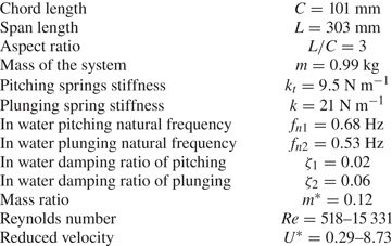
The experiments were conducted in a recirculating water tunnel equipped with a test section of dimensions  $0.45\ {\rm m} \times 0.45\ {\rm m} \times 1.5\ {\rm m}$. The turbulence intensity of the tunnel was less than 1 % at velocities up to
 $1\ {\rm m}\ {\rm s}^{-1}$. A rigid flat plate, fabricated from transparent acrylic was used in these experiments. This plate had a chord length of
 $C = 101\ {\rm mm}$ and a span of
 $L = 303\ {\rm mm}$, yielding an aspect ratio of
 $AR = L/C = 3$. The plate's thickness-to-chord ratio was 6.25 %, and its mass ratio,
 $m^{*} = 4m / {\rm \pi}\rho C^{2}$, was calculated to be 0.12. Here,
 $m$ denotes the total moving mass of the system, and
 $\rho$ represents the flow density.
The schematic of the experimental set-up is presented in figure 1. The system was designed to grant the plate two DoFs, allowing for pitching and plunging motions. The plate was mounted to a cart, which was affixed to an air-bearing system to facilitate minimal friction and enable oscillation in the plunging direction. To accommodate pitching oscillation, two springs were positioned at equal distances from the plate's axis of rotation. This axis, serving as the pivoting point, was located such that the centre of rotation and the centre of gravity coincided, ensuring a balanced rotation of the plate. The smooth torsional motion was achieved by using two ball bearings to secure two shafts attached to the plate in position. The experimental system was meticulously designed to enable independent control and restriction of each DoF. For example, when the experiment aimed to investigate pure pitching motion (1DoF), precise adjustments were implemented to restrict the plunging motion effectively, ensuring a focused examination of the desired oscillation. In instances where the experiment required a single DoF, specifically focusing on pure pitching, the system was adjusted to restrict the plunging motion.
Schematic of the experimental apparatus set-up.

The plate's plunging displacement was recorded using a laser displacement sensor (Panasonic HL-G1 Series). The pitching displacement, on the other hand, was captured through a Miniature Rotary Magnetic Encoder (Rotary and Linear Motion Sensors RM08 model). The encoder offers the advantages of high-speed operation, non-contact measurements, the absence of friction and a precision of  $\pm 0.3^{\circ }$. Data capturing the oscillations of the plate were collected at a rate of 500 Hz over a duration of 240 s. This duration ensured the recording of at least 40 oscillation cycles, which was important in verifying that the system had achieved a steady state. For a comprehensive understanding of the dynamics of the system, we collected and analysed data for such an extended period, even when the data did not show a regular pattern.
The normalised height,  $H^*$, was determined by dividing the resting height,
 $H_o$, by the plate's thickness,
 $t$. The resting height,
 $H_o$, was obtained by measuring the distance from the water surface to the upper surface of the plate, as shown in figure 1. This study covered a wide range of submerged heights for
 $H^*$ values from 26 down to 1. Adjustments to decrease
 $H^*$ were achieved by elevating the set-up and modifying the mounting point between the support arms and the air bearings in tandem. By doing so, it ensured that the total moving mass of the system remained unchanged.
To find the two natural frequencies and damping ratios of the system in each DoF, we performed free decay tests in still water and air. This involved initialising the system with a certain displacement, allowing it to oscillate freely, and collecting the oscillation amplitude data. We then further analysed the collected signal using the fast Fourier transform (FFT), and calculated the amplitude of the oscillations using the root-mean-square (r.m.s.) value of the recorded displacement signals. The intentional selection of plunging and pitching spring stiffness, crucial in establishing the natural frequency ratio in our study, was purposeful. Our goal was to deliberately position the occurrence of limit cycle oscillations within a range of flow velocities where both qualitative and quantitative flow visualisations could be conducted confidently. This careful selection strategy allowed us to effectively capture and analyse fluid–structure–surface interactions under low-flow-velocity conditions. Nevertheless, studies exclusively examining the effect of frequency ratio on the FIV response in 2DoF systems have indicated a significant influence on various aspects of their response, such as amplitude, frequency and the onset of oscillation (Poirel & Price Reference Poirel and Price2003; Zhao, Zhang & Tan Reference Zhao, Zhang and Tan2009; Menon & Mittal Reference Menon and Mittal2019; Mousavisani et al. Reference Mousavisani, Chowdhury, Samsam-Khayani, Samandari and Seyed-Aghazadeh2022). We used the pitching natural frequency in still water at  $H^*=26$ to calculate the reduced velocity, defined as
 $U^*={U}/{f_{n1}C}$, where
 $U$ is the flow velocity, and
 $f_{n1}$ is the pitching natural frequency of the system. During these tests, we kept the water level constant and gradually increased the flow velocity from 0 to
 $0.3\ {\rm m}\ {\rm s}^{-1}$ in small steps of
 $0.003\ {\rm m}\ {\rm s}^{-1}$. We measured the cross-flow response of the system for the Reynolds number range of
 $Re=518\unicode{x2013}15\,331$, corresponding to a reduced velocity range of
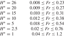
 $U^*=0.29\unicode{x2013}8.73$. Table 1 includes the system properties such as the natural frequencies and damping ratios from free decay tests, as well as the test matrix and dimensionless system parameters. We have also calculated the Froude number (denoted as
 $Fr=U/\sqrt {gH_o}$, where
 $U$ is the cross-flow speed,
 $g$ the gravitational acceleration and
 $H_o$ is the submerged height) by considering the gap between the upper surface of the plate at
 $\theta =0 ^\circ$ and the still water free surface. This analysis covered various submerged heights across the entire range of tested flow velocities, as detailed in table 2. It is important to note that, for this calculation, we did not consider the plate's oscillation or the deformation of the free surface. Defining the Froude number in our experiment presented challenges, primarily due to the temporal and local variations in the gap between the structure and the deformed free surface during occurrences of limit cycle oscillations. This was evident in the changing distance between the leading edge of the plate and the free surface throughout the oscillation period.
Experimental parameters and test plate's structural characteristics.
Froude number based on submerged heights at still water for various flow velocities.
2.2. Qualitative and quantitative flow visualisation
Vortex dynamics were explored through both qualitative and quantitative flow visualisation experiments. The hydrogen bubble visualisation technique was employed for qualitative flow visualisation. A platinum wire with a diameter of  $0.0508$ mm was strung perpendicular to the flow and the spanwise length of the flat plate over the test section. A 50–100-V, 2-A power supply positively charged a graphite plate to serve as the anode, while the platinum wire served as the cathode. The potential difference between them led to the formation of hydrogen bubbles on the platinum wire. Once their diameter exceeded that of the wire, the bubbles split from it, forming a bubble film that was utilised to observe the vortex patterns over and in the wake of the plate. Instantaneous wake structure was recorded from the side view using a high-speed camera (Victorem 32B216MCX), which captured images at 180 frames per second at a spanwise location of
 $z=0.2$ along the span of the plate measured from the centre of rotation, where
 $z$ is the dimensionless spanwise location normalised by the plate's span length. Uniform lighting conditions were ensured by installing light-emitting diode (LED) lighting at an angle underneath and above the test section to illuminate the bubble sheet.
For the quantitative flow measurement, the time-resolved volumetric particle tracking velocimetry (TR-PTV) approach was used. This allowed for the quantification of the flow field dynamics over the flat plate at sample-reduced velocities. Time-resolved measurements of the flow field dynamics were conducted using a state-of-the-art three-dimensional Lagrangian particle tracking velocimetry system, Shake-the-Box (LaVision Inc., Ypsilanti, MI, USA). The Shake-The-Box system, which includes a ‘MiniShaker’ integrated camera system (using four cameras with  $8\ {\rm mm}$ lenses and
 $121$ frame per second capturing rate) and a flashlight LED array, was used for recording and illuminating the seeding particles, respectively. The seeding particles were high-quality hollow glass polyamide spheres with a nominal diameter of
 $60\,\mathrm {\mu }{\rm m}$. At each sample's reduced velocity, multiple distinct subsets of 3878 images, corresponding to
 $32$ s of measurement (which encompass a minimum of 8 oscillation cycles of the plate), were acquired. The spatial resolution of the image sensor is
 $1984\times 1264\ {\rm pix}^2$. The vector grid resolution of the PTV data is 32 voxels:
 $6.36\ {\rm mm}\times 6.36\ {\rm mm}\times 6.36\ {\rm mm}$. The total field of view is about
 $[x\times y\times z]= 457\ {\rm mm}\times 301\ {\rm mm}\times 120\ {\rm mm}$ which corresponds to
 $4.5C\times 3C\times 1.2C$ where
 $C$ is the chord length of the plate. Figure 1 shows the schematic of the PTV measuring set-up, which includes the positions of the LED flashlight and Minishaker cameras. Further details on the hydrogen bubbles and 3D-PTV visualisation techniques employed in this study can be found in our previous work (Mousavisani et al. Reference Mousavisani, Chowdhury, Samsam-Khayani, Samandari and Seyed-Aghazadeh2022).
3. Results
3.1. Structural response of the system
3.1.1. Plate with single DoF
The first series of experiments were conducted with a rigid flat plate having a single DoF (1DoF), which allowed for pure pitching oscillation. This configuration was tested for an initial angle of attack (AoA) of zero for the plate. The choice of a zero AoA was significant because varying initial AoAs can lead to substantial shifts in bifurcation behaviours (Dugundji Reference Dugundji2008; Razak, Andrianne & Dimitriadis Reference Razak, Andrianne and Dimitriadis2011; Menon & Mittal Reference Menon and Mittal2019). The flow velocity was gradually increased up to a maximum of  $0.30\ {\rm m}\ {\rm s}^{-1}$. The amplitude of oscillation,
 $\theta$, was determined by computing the r.m.s. value of the pitching amplitudes. Meanwhile, the time-averaged pitching angle was defined as
 $\bar {\theta }$. Figure 2 shows the bifurcation diagram for the 1DoF system at various submerged heights (
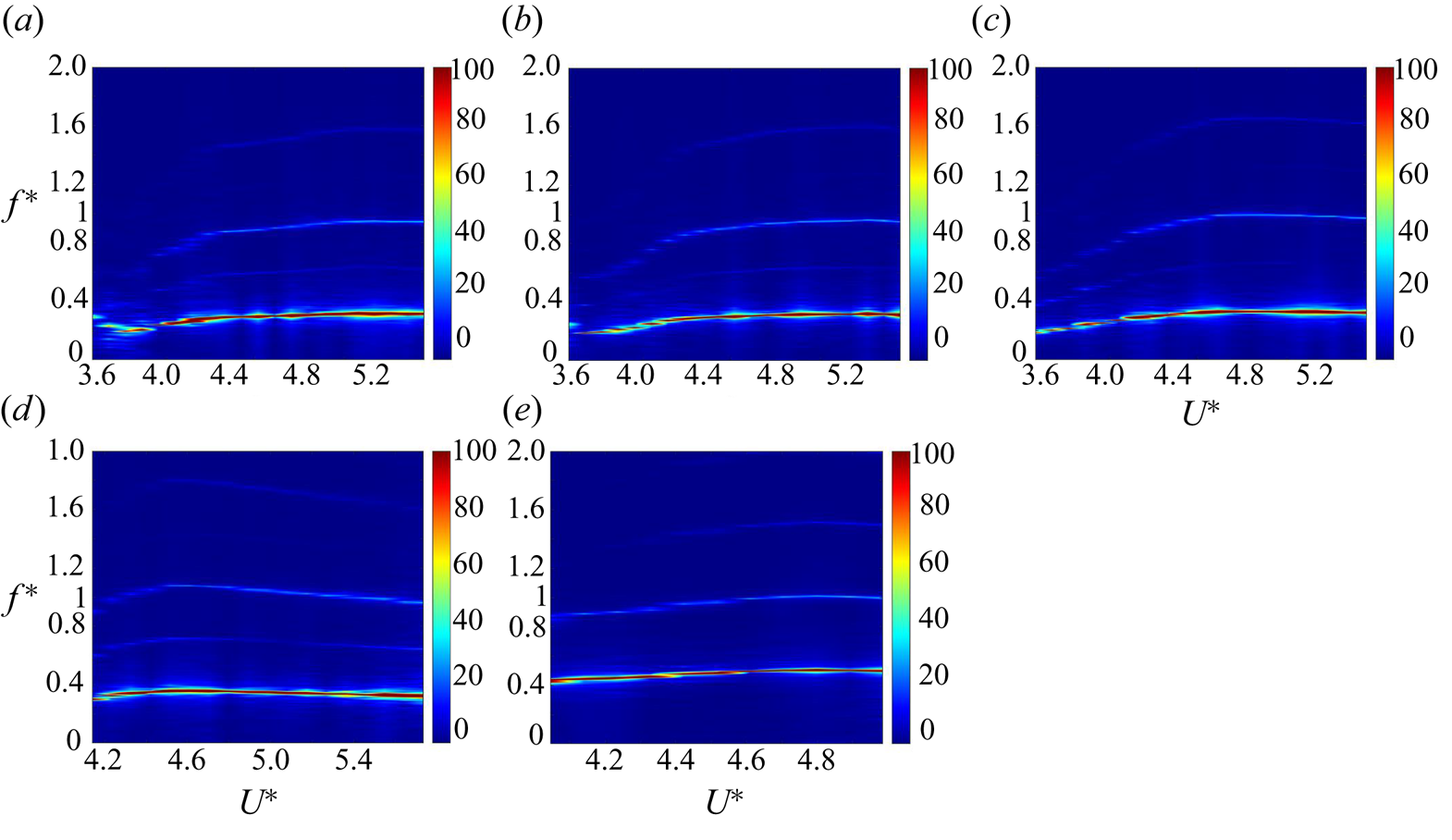
 $H^*$). This diagram plots the oscillation amplitude and mean angle of the pitching response against the reduced velocity at each submerged height of the plate. The normalised frequency content of the response, as analysed through the FFT against reduced velocity for various submerged heights, is shown in figure 3. The pitching natural frequency in still water at
 $H^*=26$ was used to normalise the frequency content.
Response of the 1DoF system: (a) amplitude of pitching oscillations as a function of reduced velocity and (b) mean pitching value as a function of reduced velocity.

Frequency content of the 1DoF system (pitching oscillation) as a function of reduced velocity for different submerged heights: (a)  $H^*=26$, (b)
 $H^*=20$, (c)
 $H^*=15$, (d)
 $H^*=10$ and (e)
 $H^*=5$.
Based on the reduced velocities tested, the behaviour of the flat plate can be categorised into four distinct phases:
(i) a steady-state condition where the initial AoA is preserved at low flow velocities;
(ii) a divergence instability where a minor static deflection is observed;
(iii) self-sustained flow-induced oscillation or the limit cycle of oscillation (LCO); and
(iv) a second range of divergence instability in which the LCO is damped out.
At submerged heights of  $H^*=26$ and
 $20$, the plate demonstrated stability, maintaining its initial AoA at lower reduced velocities. A static deflection at the first critical reduced velocity of
 $U^*=1.98$ marked the onset of the initial divergence instability, reaching a maximum amplitude of
 $\theta =6.5^\circ$ when the flow velocity increased up to
 $U^*=3.48$. The plate then starts a self-excited oscillation, also known as a LCO, within a limited reduced velocity range of
 $U^*=3.58\unicode{x2013}5.55$. The oscillation of the flat plate ceased at the third critical reduced velocity of
 $U^*=5.55$, and a second range of divergence instability occurred, with the static deflection amplitude increasing with reduced velocity, as shown in figure 2(b).
The mean value initially increased for these two deeply submerged heights,  $H^*=26$ and
 $20$, soon after the LCO's onset, but it eventually dropped to a maximum value of
 $-5.5^\circ$. This pattern, indicating nearly symmetric oscillation in upstroke and downstroke motions, persisted until the third critical reduced velocity. At this point, the LCO was damped out, giving way to the second range of divergence instability. The mean divergence value subsequently increased from
 $30^\circ$ to
 $76^\circ$. As shown in figure 3(a,b), an increase in flow velocity led to a rise in the oscillation frequency until it nearly plateaued at higher reduced velocities. Concurrently, the amplitude of the oscillation also exhibited an ascending trend. A superharmonic frequency content four times the initial oscillation's frequency was observed at higher reduced velocities. The FFT analysis revealed the presence of frequency components at two and three times the fundamental frequency. However, these higher harmonics exhibited significantly smaller amplitudes, making them barely distinguishable in the FFT contour.
At  $H^*=15$, the onset of divergence instabilities was observed to shift slightly to higher reduced velocities, specifically at
 $U^*=2.55$, indicating a change in the deflection angle to
 $\theta =1^\circ$. However, the onset and amplitude of LCO remained consistent with those observed at
 $H^*=26$. Similarly to the larger submerged heights, the mean oscillation amplitude value was near zero, reaching a maximum value of
 $-4^\circ$. The FFT contour in figure 3(c) suggests that the free surface effect on the system's frequency content was minimal at this submerged height. Thus, it can be concluded that the FIV behaviour of the system remains consistent for deeply submerged cases (i.e.
 $H^*\ge 15$) for the 1DoF system.
In what follows, the general behaviour of the 1DoF system at  $H^*=26$ is discussed through five representative samples of reduced velocities. The plate's response at five reduced velocities,
 $U^*=3.58$,
 $U^*=3.95$,
 $U^*=4.32$,
 $U^*=4.70$ and
 $U^*=5.27$ at
 $H^*=26$, is shown in the time history, frequency plot, scalogram and phase-plane plots shown in figure 4. Wavelet transform of the response at different submerged heights and reduced velocities help visualise the oscillatory dynamics of the systems in the scalograms, with the
 $x$-axis denoting time and the
 $y$-axis representing the scales of equivalent frequencies. The two-dimensional state-space is constructed using the state variables of the oscillation amplitudes (
 $\theta$ and
 $y$) and their first derivatives (
 $\dot {\theta }$ and
 $\dot {y}$). The frequency content and scalogram plots are normalised using the pitching natural frequency in still water at
 $H^*=26$. As shown in figure 4, the system's time history at these reduced velocities is periodic, evidenced by a single closed loop in the phase-plane plots. The frequency and scalogram plots highlight a dominant frequency,
 $f^*$, representing the spectral content of steady-state oscillations within this range of reduced velocities. As the reduced velocity increases, the system's response is influenced not only by the main harmonic but also by low amplitude even and odd superharmonic frequencies. The presence of these superharmonics is confirmed by minor distortions in the phase-plane plots. At a reduced velocity of
 $U^*=3.95$, weak second and third peaks were observed at two and three times the dominant oscillation frequency, respectively (figure 4b). The relative strength of the second harmonic decreases compared with the third harmonic as the reduced velocity increases. From
 $U^*=4.32$ to
 $U^*=5.27$, a modest second peak is observed at four times the frequency of the dominant oscillation figure 4(c–e). Similar observations of superharmonic frequencies contributing to the spectral content, alongside the main frequency of self-sustained oscillation of an airfoil, have also been reported by Poirel, Harris & Benaissa (Reference Poirel, Harris and Benaissa2008) and Yuan, Poirel & Wang (Reference Yuan, Poirel and Wang2013).
Oscillation response of the 1DoF system at  $H^*=26$ for different reduced velocities. Each column represents a specific reduced velocity:
 $U^*=3.58$ (a i–a iii),
 $U^*=3.95$ (b i–b iii),
 $U^*=4.32$ (c i–c iii),
 $U^*=4.70$ (d i–d iii) and
 $U^*=5.27$ (e i–e iii). The figure includes sample time histories, FFT plots, scalograms and phase planes corresponding to each reduced velocity.
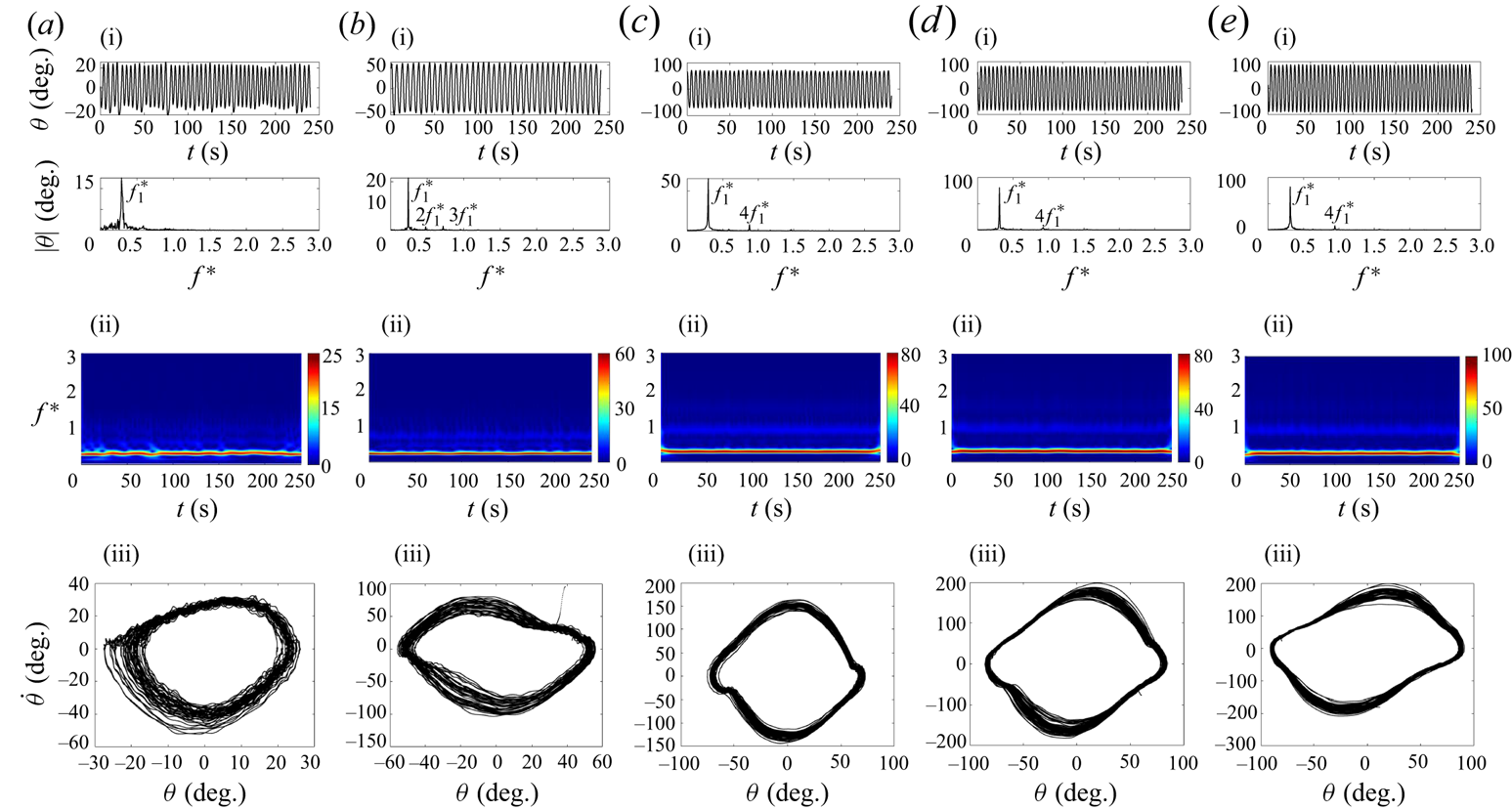
Figure 2 shows that as the submerged height decreases to  $H^*\le 10$, the effect of the free surface on the plate's response becomes more significant. The oscillation amplitude and mean value graphs in figure 2 show that as
 $H^*$ decreases than this critical submerged depth
 $(H^*_{cr})$, the instabilities move to higher reduced velocities. In addition, there's a decrease in the size and range of the LCOs, as well as a decrease in the mean value of the oscillation amplitude and the second range of divergence instability. The FFT content in figure 3(d) shows that the oscillation frequency starts at a higher value for
 $H^*\le 10$ than for
 $H^*\ge H^*_{cr}$ (
 $H^*=26$,
 $20$ and
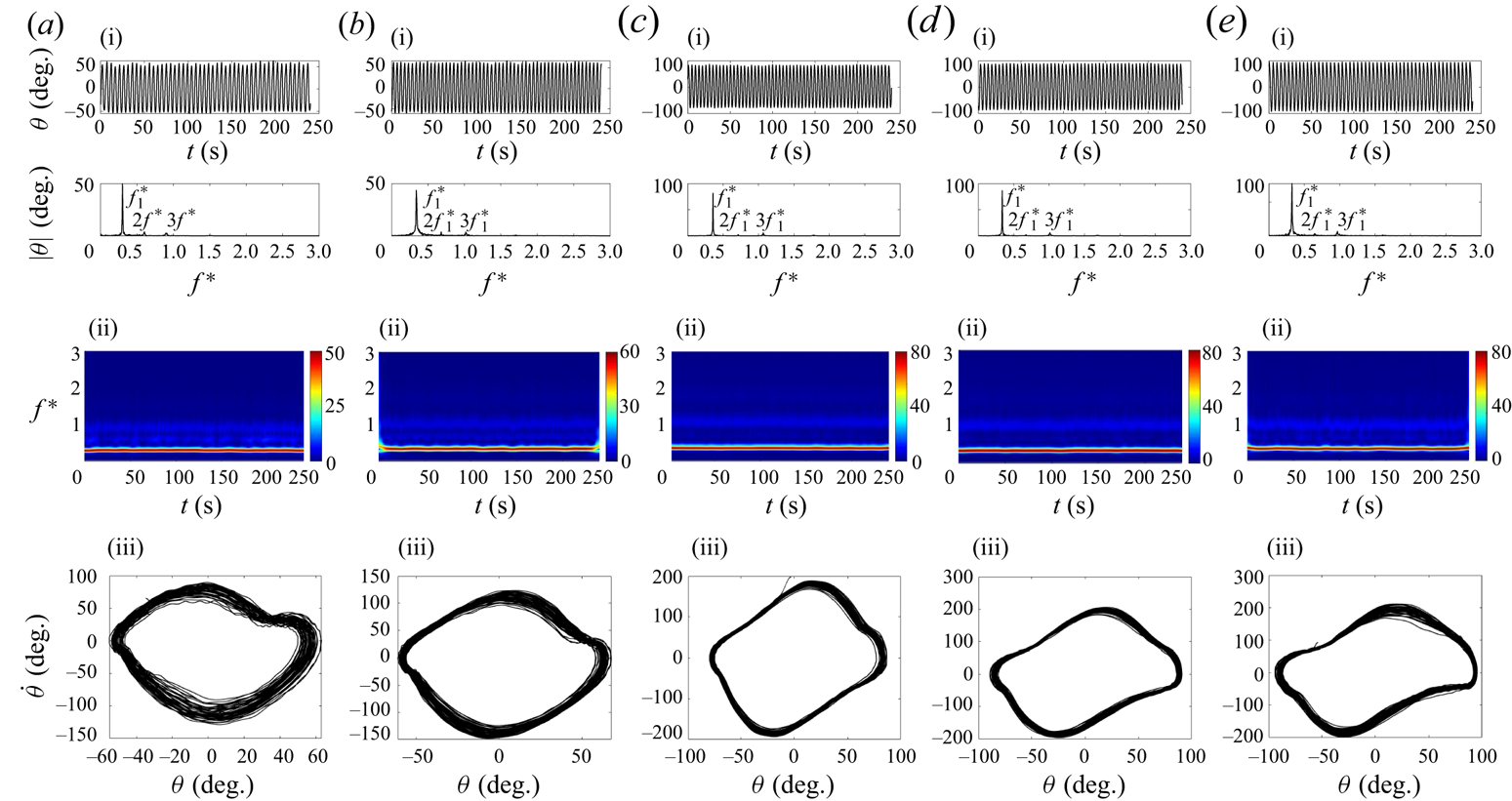
 $15$), with contributions from the superharmonic frequencies. Figure 5 presents similar plots to figure 4, but for reduced velocities of
 $U^*=4.14$,
 $U^*=4.32$,
 $U^*=4.80$,
 $U^*=5.27$ and
 $U^*=5.64$ at
 $H^*=10$. These plots indicate that the system's response at these reduced velocities remains single harmonic, as confirmed by the time history and frequency plots. However, small peaks are observed at two and three times the initial oscillation frequency, which are present throughout the entire oscillation range. The phase-plane plots exhibit slight distortions from a perfect ellipse shape, which are likely due to the influence of the superharmonic frequencies.
Sample time histories, FFT plots, scalograms and phase planes for oscillation response of the 1DoF system at  $U^*=4.14$ (a i–a iii),
 $U^*=4.32$ (b i–b iii),
 $U^*=4.80$ (c i–c iii),
 $U^*=5.27$ (d i–d iii) and
 $U^*=5.64$ (e i–e, iii) at
 $H^*=10$.
The FIV response at a submerged height of  $H^*=5$ differs considerably from other submerged heights we have discussed. We observed a substantial drop in the oscillation amplitude, a marked decrease in the LCO area and a shift of the LCO endpoint to lower reduced velocities (
 $U^*=5.08$). This is in contrast to
 $H^*=10$, where the LCO endpoint shifted to higher reduced velocities (
 $U^*=5.74$) compared with deep submergence conditions. The first range of divergence instability began at
 $U^*=3.02$ with an AoA of
 $\theta =5^\circ$, which increased up to an
 $\theta$ of
 $6.5^\circ$ at
 $U^*=3.95$. Unlike cases where
 $H^*\ge 10$, the plate, due to the free surface boundary on the upstroke motion, demonstrated a significant increase in the mean amplitude of oscillation. This increase, shown by a non-zero negative value towards the downstroke motion, highlights the asymmetry of the oscillation.
The mean amplitude of oscillation started at  $\bar {\theta }=-7.5^\circ$ and grew to
 $\bar {\theta }=-24.5^\circ$, a clear contrast to the maximum positive mean value of
 $\bar {\theta }=65^\circ$ at
 $H^*\ge {10}$. Because the plate's motion was limited by the free surface boundary, the second range of divergence angle did not increase as much as in the cases with greater submerged heights. Indeed it started at a positive value of
 $4.5^\circ$ and reached a peak of
 $16\,^\circ$, before dropping to
 $8.5^\circ$ as the reduced velocity increased, as shown in figure 2(b). According to the FFT content in figure 3, the dominant oscillation frequency at
 $H^*=5$ nearly doubled compared to
 $H^*\ge 15$, along with the addition of superharmonic frequencies.
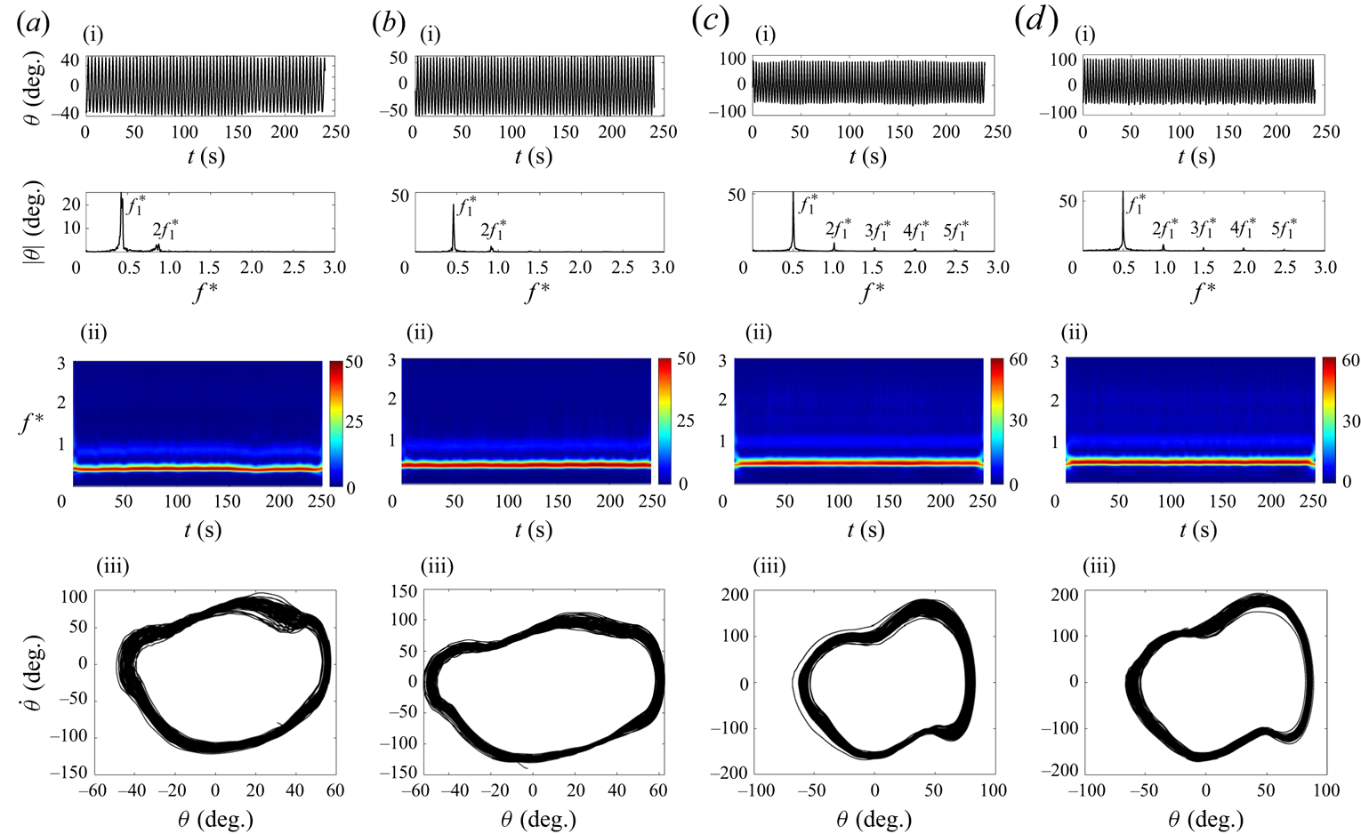
Figure 6 provides similar plots to figure 4, but for reduced velocities of  $U^*=4.05$,
 $U^*=4.32$,
 $U^*=4.80$ and
 $U^*=4.98$ at
 $H^*=5$. The single closed loop in the phase plane of figure 6 indicates periodic oscillations. At
 $U^*=4.05$ and
 $U^*=4.32$, a weak peak was detected at twice the dominant oscillation frequency, whereas higher reduced velocities led to a modest contribution from superharmonic frequencies, such as those three, four and five times the dominant frequency. These plots show how the plate's interaction with the free surface led to the creation of superharmonic frequencies. This phenomenon is further explored in the discussion of flow visualisation using three-dimensional vorticity, hydrogen bubble and POD analysis.
Sample time histories, FFT plots, scalograms and phase planes for oscillation response of the 1DoF system at  $U^*=4.05$ (a i–a iii),
 $U^*=4.32$ (b i–b iii),
 $U^*=4.80$ (c i–c iii) and
 $U^*=4.98$ (d i–d iii) at
 $H^*=5$.
Near the free surface, at submerged heights as low as  $H^*=2.5$ and
 $1$, the LCO was completely suppressed across all tested ranges of reduced velocity, as shown in figure 2. The mean value,
 $\bar {\theta }$, at these submerged heights can be seen in figure 2(b). As the flow velocity was increased, the divergence instability initially seen at
 $U^*=2$ (with a value of
 $\bar {\theta }=2^\circ$) increased to
 $\bar {\theta }=4.7^\circ$ at
 $U^*=2.73$. As the reduced velocity was increased further, the plate developed a negative divergence angle (directed towards the downstroke direction) due to the close proximity to the free surface. This angle increased as the flow velocity was increased, reaching up to
 $\bar {\theta }=-11^\circ$ for
 $H^*=1$ and
 $\bar {\theta }=-18.8^\circ$ for
 $H^*=2.5$. The plate demonstrated a higher negative divergence angle at
 $H^*=2.5$ compared with
 $H^*=1$, given that it was positioned further below the free surface at
 $H^*=2.5$.
3.1.2. Plate with two DoFs
In this section, the behaviour of a plate with both pitching and plunging DoFs is discussed. Initially, the plate was deeply submerged in still water with a zero AoA. To investigate the effects of  $H^*$, the plate was gradually brought closer to the free surface, with the flow velocity incrementally increasing by
 $0.003 \ {\rm m}\ {\rm s}^{-1}$ up to a maximum of
 $0.30 \ {\rm m}\ {\rm s}^{-1}$, similar to the approach used in the 1DoF system. The plunging and pitching responses of the system denoted as
 $y$ and
 $\theta$, respectively, were recorded using both the laser displacement sensor and the magnetic encoder. The dimensionless amplitude of the plunging oscillation,
 $y^*$, was normalised using half the chord length of the plate (
 $C/2=0.0508\ {\rm m}$). In line with the approach used for the 1DoF system,
 $\bar {\theta }$ and
 $\bar {y}^*$ were defined as the mean values of the pitching angle and plunging amplitude, respectively.
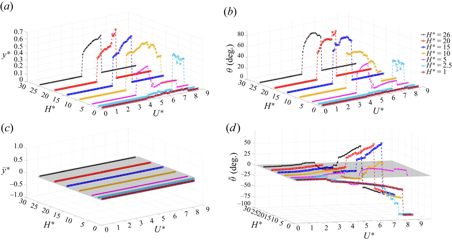
Figure 7(a,b) shows the bifurcation diagram for the 2DoF system at various submerged heights ( $H^*$). In these figures, the plunging and pitching amplitude responses are plotted against the reduced velocity. Figure 7(c,d) shows
 $\bar {y}^*$ and
 $\bar {\theta }$ for different submerged heights as the reduced velocity (
 $U^*$) varies. The frequency content of the response in both the pitching and plunging directions vs reduced velocity for various submerged heights is presented in figure 9. As with the 1DoF plate, as reduced velocities increase, the plate first experiences divergence instability, followed by the LCO, the amplitude of which grows with the increasing flow velocity. At the third critical reduced velocity, the LCOs were entirely suppressed.
Amplitude and mean value of plunging oscillations (a,c) and pitching oscillations (b,d) vs reduced velocity in the 2DoF system.
At this point, it is important to note that typically, in a system with two DoFs such as a foil or flat plate with pitching and plunging modes, the start of LCOs is explained by the synchronisation of the modal frequencies (Tripathi et al. Reference Tripathi, Shreenivas, Bose, Mondal and Venkatramani2022). In this context, the modal frequencies refer to the frequencies of the pitching and plunging oscillations. This synchronisation could be a feature of the nonlinear nature of these frequencies. To gain insight into synchronisation and the frequencies of oscillation, we conducted a comprehensive study considering both pitching and plunging directions. The synchronisation analysis involved measuring the oscillation frequencies in various scenarios, including 1DoF (pitching or plunging) and 2DoF (pitching and plunging) modes, as illustrated in figures 8(a) and 8(b), respectively. To perform these measurements, we manually perturbed the system at each increment of the cross-flow speed, similar to the free decay tests. The flat plate oscillation was then allowed to decay in both the 1DoF and 2DoF systems. Starting from zero cross-flow speed, we systematically increased the flow speed and continued the decay tests until we reached the second critical reduced velocity of  $U^*=3.58$, at which the onset of LCO was observed in the deeply submerged cases, as discussed previously. In the 1DoF system, figure 8(a) demonstrates that the plunging frequency remained constant, whereas the pitching frequency decreased as the cross-flow speed increased until the onset of LCO in the pure pitching configuration. On the other hand, figure 8(b) shows the evolution of frequency coalescence between the pitching and plunging modes in the 2DoF system. In this case, the plunging frequency remained nearly unchanged, whereas the pitching frequency decreased with increasing flow velocity until the onset of oscillation. As we approached the second critical reduced velocity, the plunge frequency converged with the pitch frequency. Based on this observation, it can be inferred that the plunging DoF acts as a follower, being driven by the pitching DoF. In simpler terms, the pitch motion appears to dictate the LCO frequency of the 2DoF system, as the LCO frequency aligns more closely with the pitch frequency.
Variation in dominant frequencies of pitch and plunge responses vs reduced velocity at  $H^*=26$; (a) 1DoF systems and (b) 2DoF system.

Frequency content vs reduced velocity for pitching and plunging oscillations in the 2DoF system at various submerged heights:  $H^*=26$ (a),
 $H^*=20$ (b),
 $H^*=15$ (c),
 $H^*=10$ (d),
 $H^*=5$ (e) and
 $H^*=2.5$ (f). Plunging FFT contours are displayed in (a i,b i,c i) and (d i,e i,f i), whereas (a ii,b ii,c ii) and (d ii,e ii,f ii) show the corresponding pitching FFT contours.
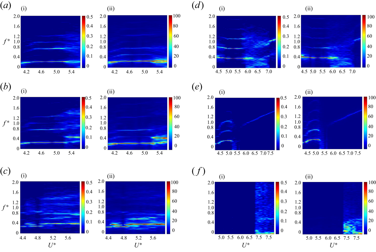
The first set of experiments in the 2DoF system was conducted at a submerged height of  $H^*=26$, which corresponds to a deeply submerged condition in the 1DoF tests. As shown in figure 7, at this submerged height, an increase in the flow velocity causes the static divergence of the plate at a reduced velocity of
 $U^*=1.98$ with an angle of
 $1^\circ$. The static divergence value increases to
 $6.5^\circ$ as the flow velocity increases to
 $U^*=3.95$. The oscillation in the 2DoF system starts at
 $U^*=4$, compared with
 $U^*=3.57$ in the 1DoF system, indicating a slight shift of the LCO onset to a higher reduced velocity. The frequency contours vs reduced velocity for the plunging and pitching directions at
 $H^*=26$ are shown in figure 9(a i,a ii). From these figures, it can be seen that the dominant oscillation frequency increases from
 $f^*=0.18$ to
 $f^*=0.25$ as the reduced velocity increases up to
 $U^*=4.4$. This dominant frequency then remains steady with further increases in reduced velocity, until a wide range of frequencies emerges. Superharmonic frequencies, both even and odd, such as
 $3f^*_1$,
 $4f^*_1$, and
 $5f^*_1$ were observed in both the plunging and pitching responses. These superharmonic frequencies were more pronounced in the plunging response than in the pitching response. Figure 7(c,d) shows that the plate in the pitching direction exhibited a non-zero negative mean value during the oscillation up to
 $\theta =-7.5^\circ$, whereas the plunging oscillation maintained a zero mean value. Even though the LCO was completely damped out at the third critical flow velocity of
 $U^*=5.65$, a second range of static divergence was observed. The amplitude of this instability increased up to
 $\theta =41.5^\circ$ at
 $U^*=7.32$, after which the static divergence angle turned negative and increased to
 $\theta =-69^\circ$.
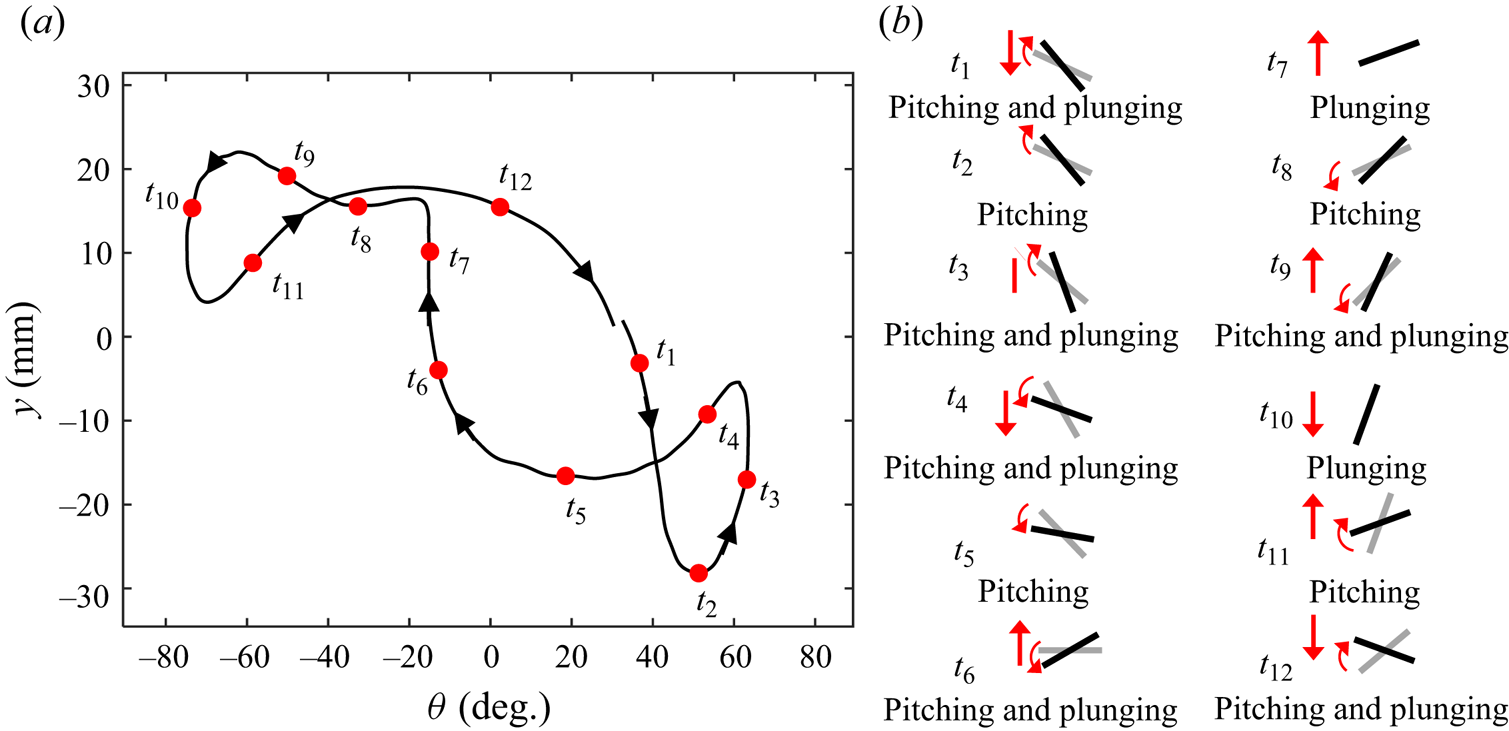
A schematic representation of the general behaviour of the oscillating 2DoF plate alongside the pitching vs plunging displacement at  $H^*=26$ and
 $U^*=4.32$ is presented in figure 10. The solid line in figure 10(a) shows the relationship between pitching and plunging displacements for a sample reduced velocity of
 $U^*=4.70$ at a deep submergence height of
 $H^*=26$. Time intervals of
 $t_1$ to
 $t_{12}$ show the corresponding phase of the plate during oscillation, where the grey solid line represents the previous state of the plate at each time step, as shown in figure 10(b). This figure reveals a highly periodic response that exhibits three closed loops, suggesting a synchronisation phenomenon.
(a) Pitching vs plunging displacement at  $H^*=26$ and
 $U^*=4.32$ and (b) schematic of the oscillating 2DoF plate at
 $H^*=26$. The grey solid lines in (b) represent previous state of the plate at each time.
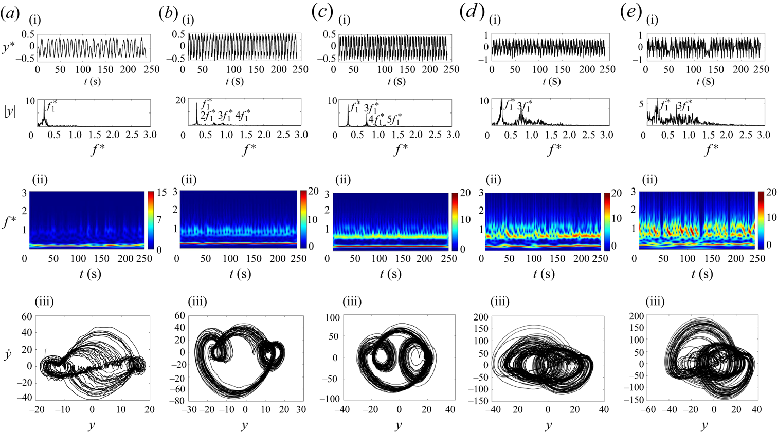
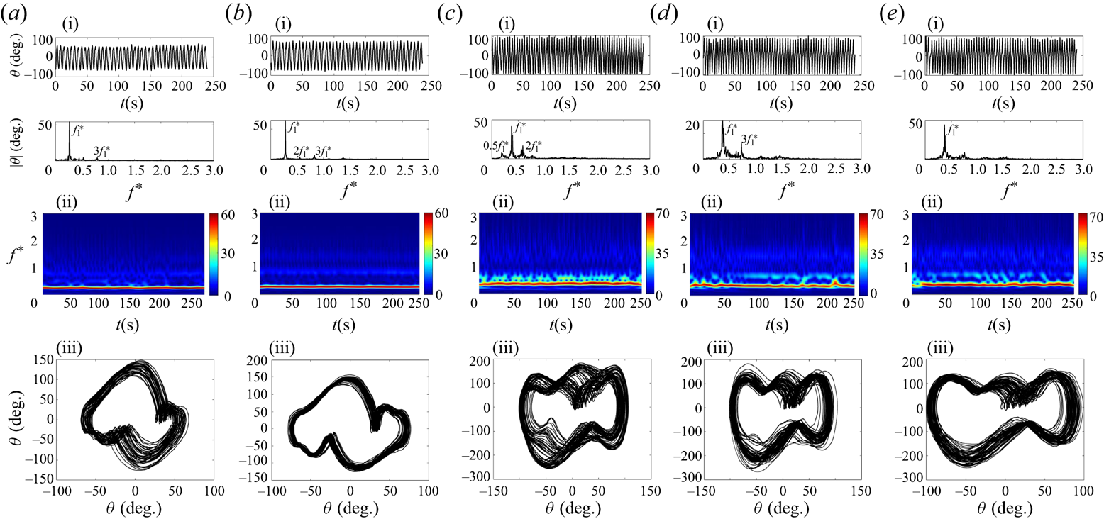
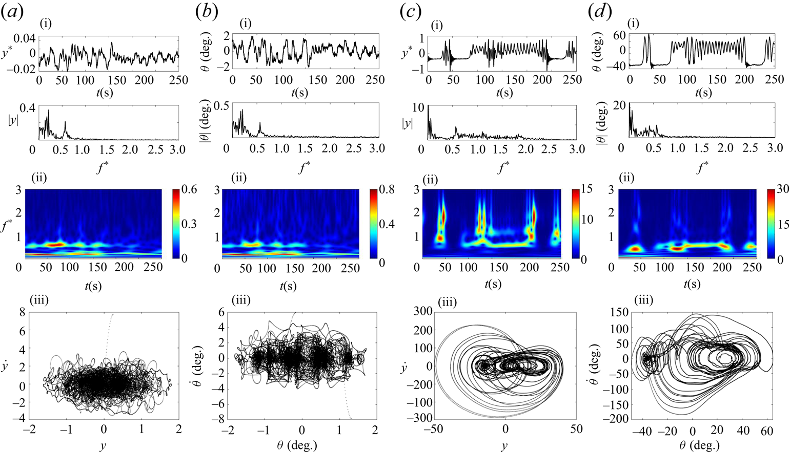
In the following section, the general behaviour of the 2DoF system at  $H^*=26$ is discussed through the examination of five representative samples of reduced velocities. Time histories, frequency plots, scalograms and phase-plane plots of the plate's plunging and pitching responses at
 $H^*=26$ are displayed in figures 11 and 12. These figures correspond to five reduced velocity samples:
 $U^*=4.05$,
 $U^*=4.32$,
 $U^*=4.80$,
 $U^*=5.26$ and
 $U^*=5.55$. As shown in figures 11 and 12, at the onset of LCO, the system's response in both directions primarily comprises a single dominant frequency, that is also confirmed by the scalogram contour and the single closed-loop cycle in the phase-plane plot. With increasing flow velocity, the response of the 2DoF system becomes more complex, featuring superharmonic frequencies. The frequency content and scalogram of the plunging mode in figure 11 for
 $U^*=4.32$ (figure 11b i–b iii) show a single dominant frequency, with weak superharmonic frequencies. This trend is further confirmed by the phase-plane plot in figure 11(b iii), which exhibits three closed-loop cycles. A similar pattern of dominant and superharmonic frequencies is evident in both directions in figure 12, confirming the synchronisation of the plunging and pitching modes. The second peak in the frequency content and scalogram contour of the pitching mode is more pronounced compared with that in the plunging mode.
Sample time histories, FFT plots, scalograms and phase planes showing the plunging oscillation response of the 2DoF system at different reduced velocities. Columns represent  $U^*=4.05$ (a i–a iii),
 $U^*=4.32$ (b i–b iii),
 $U^*=4.80$ (c i–c iii),
 $U^*=5.26$ (d i–d iii) and
 $U^*=5.55$ (e i–e iii), all at
 $H^*=26$.
Sample time histories, FFT plots, scalograms and phase planes showing the pitching oscillation response of the 2DoF system at different reduced velocities. Columns represent  $U^*=4.05$ (a i–a iii),
 $U^*=4.32$ (b i–b iii),
 $U^*=4.80$ (c i–c iii),
 $U^*=5.26$ (d i–d iii) and
 $U^*=5.55$ (e i–e iii), all at
 $H^*=26$.

As the flow velocity further increases, as shown by the sample response at  $U^*=4.80$, superharmonic frequencies appear that are two, three, four and five times the dominant frequency. These are evident in the frequency content and scalogram contour (figures 11 and 12c i–ciii). The contribution of the third frequency, which is three times the dominant frequency in the plunging mode, increases, as shown in figure 11(c i,c ii). As the reduced velocity is increased, the system's response in both modes exhibits a broader frequency spectrum.
At the sample reduced velocities of  $U^*=5.26$ and
 $U^*=5.55$ (shown in figure 11d,e), a broad frequency response with frequencies of
 $f^*_1$ and
 $3f^*_1$ is noted in the plunging response. On the other hand, the system's pitching response presents a broad frequency spectrum with a noticeable peak at the dominant frequency of
 $f^*_1$, as seen in figure 12(d,e). Here, superharmonics contribute minimally. Compared with those in the pitching direction, the phase-plane plot in figure 11(d iii,e iii) shows a portion of the space being filled, indicative of the aperiodic response of the flat plate at these two sample reduced velocities.
Observing the oscillation amplitude and mean value in figure 7, it can be conceived that a similar trend occurs for  $H^*=20$ as compared with
 $H^*=26$, as also shown in figure 9(b i,b ii). When the reduced velocity
 $U^*\ge {5.36}$, the plate exhibits a change in both oscillation modes’ amplitude, a trend that is also observed in the frequency contour of oscillations in figure 9(b i,b ii), which also show an increase in frequency content. Much like the previous submerged height, an increase in reduced velocity results in the emergence of superharmonic frequencies in both oscillation modes, followed by aperiodic oscillation at higher reduced velocities.
As the submerged height drops below  $H^*=20$, the interaction between the free surface and the flat plate increases. When the plate is raised further to
 $H^*=15$, compared with the previous two submerged heights, the onset of oscillation and the second range of static divergence shift to a higher reduced velocity of
 $U^*=4.32$ and
 $U^*=5.92$, respectively. At a reduced velocity of
 $U^*=4.79$, a kink in the amplitude of oscillation modes coincides with an increase in the frequency content of the plunging and pitching oscillation, as shown in figure 9(c i,c ii). This is likely due to the increased interaction between the free surface and the flat plate at this submerged height.
Figures 13 and 14 show the overall behaviour of the 2DoF system at a submerged height of  $H^*=15$. These figures present the same plots as figures 11 and 12, but for five distinct reduced velocity samples:
 $U^*=4.32$,
 $U^*=4.80$,
 $U^*=5.26$,
 $U^*=5.73$ and
 $U^*=5.92$. At this lower submerged height, oscillation in both modes starts with the contribution of superharmonic frequencies, as shown in figures 13 and 14(a i–a iii). This contrasts with the behaviour observed at higher submerged heights. Frequency plots in the first row of figures 13 and 14 indicate that the dominant frequencies,
 $f^*_1$, increase in value as the reduced velocity increases, a trend also seen in the frequency contours (figure 9c i,c ii). Unlike in the
 $H^*\ge 20$ case, subharmonic frequencies are observed in the oscillation modes’ FFT contour, as shown in the reduced velocity sample of
 $U^*=5.26$. Furthermore, from
 $U^*\ge 4.90$, a broad frequency content is observed, likely due to the intensified interaction with the free surface as
 $H^*$ decreases.
Sample time histories, FFT plots, scalograms and phase planes showing the plunging oscillation response of the 2DoF system at different reduced velocities. Columns represent  $U^*=4.32$ (a i–a iii),
 $U^*=4.80$ (b i–b iii),
 $U^*=5.26$ (c i–c iii),
 $U^*=5.73$ (d i–d iii) and
 $U^*=5.92$ (e i–e iii), all at
 $H^*=15$.

Sample time histories, FFT plots, scalograms and phase planes showing the pitching oscillation response of the 2DoF system at different reduced velocities. Columns represent  $U^*=4.32$ (a i–a iii),
 $U^*=4.80$ (b i–b iii),
 $U^*=5.26$ (c i–c iii),
 $U^*=5.73$ (d i–d iii) and
 $U^*=5.92$ (e i–e iii), all at
 $H^*=15$.
As the submerged height drops to  $H^*\le 10$, the interaction between the free surface and the plate greatly intensifies. This leads to some significant changes compared to higher
 $H^*$ values: the range of LCO broadens, the amplitude of oscillation in the plunging modes increases contrary to a decrease in the pitching amplitude, and the onset of oscillation and the second range of static deflection shift to higher reduced velocities, as shown in figure 7(a,b).
Figure 9(d i,d ii) show that oscillation begins with a higher frequency than in  $H^*\ge {15}$ cases. This is seen by a major contribution of superharmonic frequencies up to
 $U^*=5.82$, at which point periodic oscillation is observed. From
 $U^*=5.82$ to
 $U^*=7.42$, non-periodic oscillations with a broad range of frequencies occur. The oscillation then dampens at
 $U^*=7.42$. Figure 7(c,d) show mean value results, indicating an increase in static divergence until the onset of LCO. This value rises from
 $\bar {\theta }=-1.5^\circ$ at
 $U^*=4.32$ to
 $\bar {\theta }=-14.5^\circ$ at a reduced velocity of
 $U^*=5.82$. Immediately after
 $U^*=5.82$, the mean angle of oscillation in the pitching mode begins to increase with a positive slope, reaching up to
 $\bar {\theta }=20^\circ$. This is where the decrease in oscillation amplitude in both directions starts. The second range of static divergence begins with a negative value and increases to
 $\bar {\theta }=-61^\circ$. At this submerged height, due to the interaction with the free surface, the mean value of oscillation reaches a maximum positive value of
 $\bar {\theta }=20^\circ$, in contrary to the small mean value for
 $H^*\ge {15}$.
To show the overall behaviour of the 2DoF system at this submerged height, we selected five samples of reduced velocities. Figure 15 presents the same plots as figures 11 and 12, but for five reduced velocity samples at  $H^*=10$:
 $U^*=4.32$,
 $U^*=5.26$,
 $U^*=5.73$,
 $U^*=6.67$ and
 $U^*=7.42$.
Sample time histories, FFT plots, scalograms and phase planes showing the plunging oscillation response of the 2DoF system at different reduced velocities. The columns represent  $U^*=4.32$ (a i–a iii),
 $U^*=5.26$ (b i–b iii),
 $U^*=5.73$ (c i–c iii),
 $U^*=6.67$ (d i–d iii) and
 $U^*=7.42$ (e i–e iii) all at
 $H^*=10$.

As figure 15(a i—a iii) show, the oscillation started with a wide range of frequencies in both oscillation modes, with peaks around  $f^*_1$ and
 $3f^*_1$. Superharmonic frequencies were observed at higher reduced velocities. The third superharmonic frequency,
 $3f^*_1$, became more prominent starting from a reduced velocity of
 $U^*=5.54$ and persisted to higher reduced velocities as shown in figure 15. From
 $U^*=5.92$ to
 $U^*=7.05$, the system's response became irregular, as also shown in the response of the system in figures 15 and 16(d), with high oscillation amplitudes observed in both modes. The system returned to a regular response from
 $U^*=7.14$ to
 $U^*=7.80$, where the frequency of
 $3f^*_1$ became dominant with a minor contribution from subharmonics and superharmonics. This is supported by the phase-plane and scalogram plots in figures 15 and 16(e), which confirm the nearly regular response of the system at the frequency of
 $3f^*_1$.
Sample time histories, FFT plots, scalograms and phase planes showing the pitching oscillation response of the 2DoF system at different reduced velocities. The columns represent  $U^*=4.32$ (a i–a iii),
 $U^*=5.26$ (b i–b iii),
 $U^*=5.73$ (c i–c iii),
 $U^*=6.67$ (d i–d iii) and
 $U^*=7.42$ (e i–e iii), all at
 $H^*=10$.

In this experiment, the LCOs region at  $H^*=5$ had the widest range of oscillation, extending from
 $U^*=4.23$ to
 $7.70$. The oscillation amplitude notably dropped at this submerged height, whereas two areas of LCO, each with high and low amplitudes, were evident. To show the typical system behaviour at
 $H^*=5$, we selected five sample reduced velocities. Figures 17 and 18 present the same plots as in figures 11 and 12 but for five reduced velocity samples of
 $U^*=4.23$,
 $U^*=4.80$,
 $U^*=5.73$,
 $U^*=6.67$ and
 $U^*=7.61$ at
 $H^*=5$.
Sample time histories, FFT plots, scalograms and phase planes showing the plunging oscillation response of the 2DoF system at different reduced velocities. The columns represent  $U^*=4.23$ (a i–a iii),
 $U^*=4.80$ (b i–b iii),
 $U^*=5.73$ (c i–c iii),
 $U^*=6.67$ (d i–d iii) and
 $U^*=7.61$ (e i–e iii) all at
 $H^*=5$.

Sample time histories, FFT plots, scalograms and phase planes showing the pitching oscillation response of the 2DoF system at different reduced velocities. The columns represent  $U^*=4.23$ (a i–a iii),
 $U^*=4.80$ (b i–b iii),
 $U^*=5.73$ (c i–c iii),
 $U^*=6.67$ (d i–d iii) and
 $U^*=7.61$ (e i–e iii) all at
 $H^*=5$.

Oscillation began with a negative mean value, indicating downward motion, in the pitching mode at  $U^*=4.23$, just after the first region of static deflection. The negative mean value continued to grow from
 $\theta =-12.80^\circ$ at
 $U^*=4.23$ to
 $\theta =-21^\circ$ at
 $U^*=5.17$, alongside an increase in the amplitude of oscillation. As shown in figure 9(e i,e ii) and two sample reduced velocities in figures 17 and 18(a,b), the system experienced periodic oscillation in this high-amplitude oscillation region, with the presence of superharmonic frequencies. Increasing the reduced velocity further from
 $U^*=5.26$ resulted in a decrease in the amplitude of oscillations until
 $U^*=5.73$, whereas the mean value of pitching oscillation rose with a positive slope. Oscillation in this region was aperiodic, as shown in figures 17 and 18(c). The mean value of pitching oscillation continued to grow, reaching a positive value until oscillation ceased at
 $U^*=7.80$, where it dropped to
 $\theta =-2^\circ$ at
 $U^*=8.73$. The amplitude of oscillation increased nearly linearly from
 $U^*=5.73$ to
 $U^*=7.80$ until the oscillation was damped. In the second region of oscillation, as shown in figure 9(e i,e ii) and the two sample reduced velocities in figures 17 and 18(d,e), the plate's periodic response resumed with the superharmonic frequency making a major contribution, which increased linearly.
The oscillation amplitude significantly reduced as  $H^*$ was decreased to
 $2.5$ and
 $1$. As shown in figure 7(a,b), the plate at
 $H^*=2.5$ showed a large amplitude of aperiodic oscillation when
 $6.95\le U^* \le 7.80$. Similar high-amplitude oscillations at low
 $H^*$ and high
 $U^*$ values for the 1DoF circular cylinder were reported by Saelim (Reference Saelim1999); Capell, Carlson & Modarres-Sadeghi (Reference Capell, Carlson and Modarres-Sadeghi2019). Figure 19 presents the same plots as figures 11 and 12, but for two reduced velocity samples of
 $U^*=4.80$ and
 $U^*=7.61$ at
 $H^*=2.5$. The frequency and phase plots shown in these figures provide conclusive evidence of the observed aperiodic oscillation. At
 $H^*=2.5$, due to the plate's proximity to the free surface, it faced downward force from the fluid flow, as evidenced by the negative mean value of oscillation across the entire range of tested reduced velocity, shown in figure 7(c,d).
Sample time histories, FFT plots, scalograms and phase planes showing the plunging (a,c) and pitching (b,d) oscillation responses of the 2DoF system at two different reduced velocities. The columns represent  $U^*=4.80$ (a i–a iii and b i–b iii) and
 $U^*=7.61$ (c i–c iii and d i–d iii), all at
 $H^*=2.5$.
As the plate was moved even closer to the free surface, at  $H^*=1$, the previously observed high amplitude of oscillation was absent, and the plate exhibited a minimal amplitude of oscillation that could be almost disregarded. It can be hypothesised that the damped oscillation at
 $H^*\le 2.5$ is due to the presence of a small volume of fluid above the plate's upper surface, resulting in weaker wake forcing, which was not powerful enough to initiate oscillation. The mean value of the second static divergence in the pitching mode for both
 $H^*=2.5$ and
 $1$ exhibited a negative value. This negative value continued to increase as the reduced velocity increased. As the plate approached the perpendicular position, indicated by the mean value of
 $\bar {\theta }=-90^\circ$ in figure 7(d), it crossed the free surface due to the small gap between the plate and the free surface at these submerged heights.
3.2. Flow field characteristics
3.2.1. Flow analysis for a plate with single DoF
This part of the study focuses on examining the three-dimensional TR-PTV and two-dimensional hydrogen bubble flow visualisation results for the 1DoF system. The structural response of this system was discussed earlier in § 3.1.1.
For a thorough understanding of the vortex structures, we used three- and two-dimensional vorticity, as well as the  $Q$-criterion representations. These tools were applied to both time-averaged and instantaneous vector fields. The
 $Q$-criterion is a method that uses the velocity gradient tensor. In this method, the velocity gradient tensor
 $\bar {D}$ is defined as
 $D_{ij}={\partial {u_i}}/{\partial {x_j}}$ (Hunt, Wray & Moin Reference Hunt, Wray and Moin1988). This second-order tensor can be split into two parts, symmetric and skew-symmetric, represented as
 $D_{ij}= S_{ij}+ \varOmega _{ij}$. Here,
 $S_{ij}=({\partial {u_i}}/{\partial {x_j}}+{\partial {u_j}}/{\partial {x_i}})/2$ is known as the rate-of-strain tensor, and
 $\varOmega _{ij}=({\partial {u_i}}/{\partial {x_j}}-{\partial {u_j}}/{\partial {x_i}})/2$ is called the vorticity tensor (Hunt et al. Reference Hunt, Wray and Moin1988). The
 $Q$-criterion is defined as the second invariant of the velocity gradient tensor:
 \begin{equation} Q= \frac{1}{2}({{\rm tr}(\bar{D})^2}-{\rm tr}(\bar{D})^2)= \frac{(|\varOmega|^2 - |S|^2)}{2}. \end{equation}
The  $Q$-criterion helps identify a vortex as a fluid region with positive
 $Q$ values. Equation (3.1) shows a local balance between shear strain rate and vorticity magnitude, defining the vortex as an area where the vorticity magnitude is higher than the magnitude of the rate of strain.
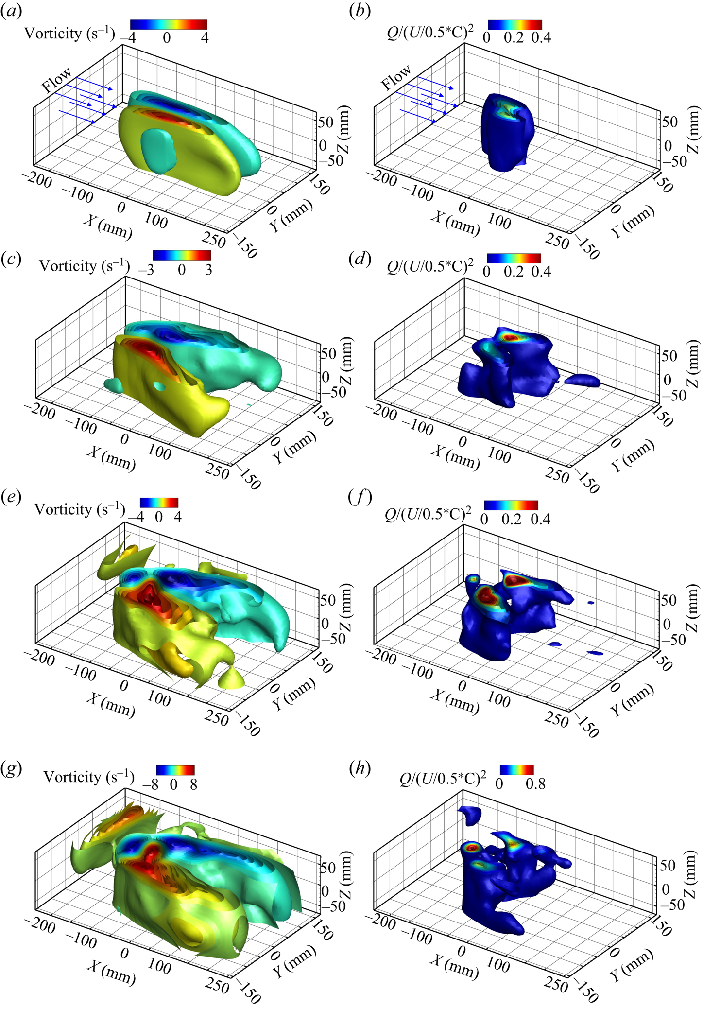
Figure 20 shows the time-averaged three-dimensional vorticity (a,d,g,j,m) and normalised  $Q$-criterion (b,e,h,k,n) of the 1DoF system at four different reduced velocities,
 $U^*=3.01$,
 $U^*=3.76$,
 $U^*=4.32$ and
 $U^*=5.26$, in the deeply submerged case of
 $H^*=26$. Figure 20(a,b) show samples of reduced velocities at which the plate underwent the divergence instabilities. Here, we observed an oblique negative vorticity in the positive
 $Y$ direction over the top surface (suction side) of the plate, compared with the positive shear layer vorticity of the bottom surface. Figure 20(c–h) presents a series of reduced velocities that demonstrate the behaviour of a plate undergoing LCO. These figures illustrate the amplification of two symmetric vortices during the upstroke and downstroke motions, which increase in size and strength with higher reduced velocities. The analysis focused on various aspects, including time-averaged vorticity,
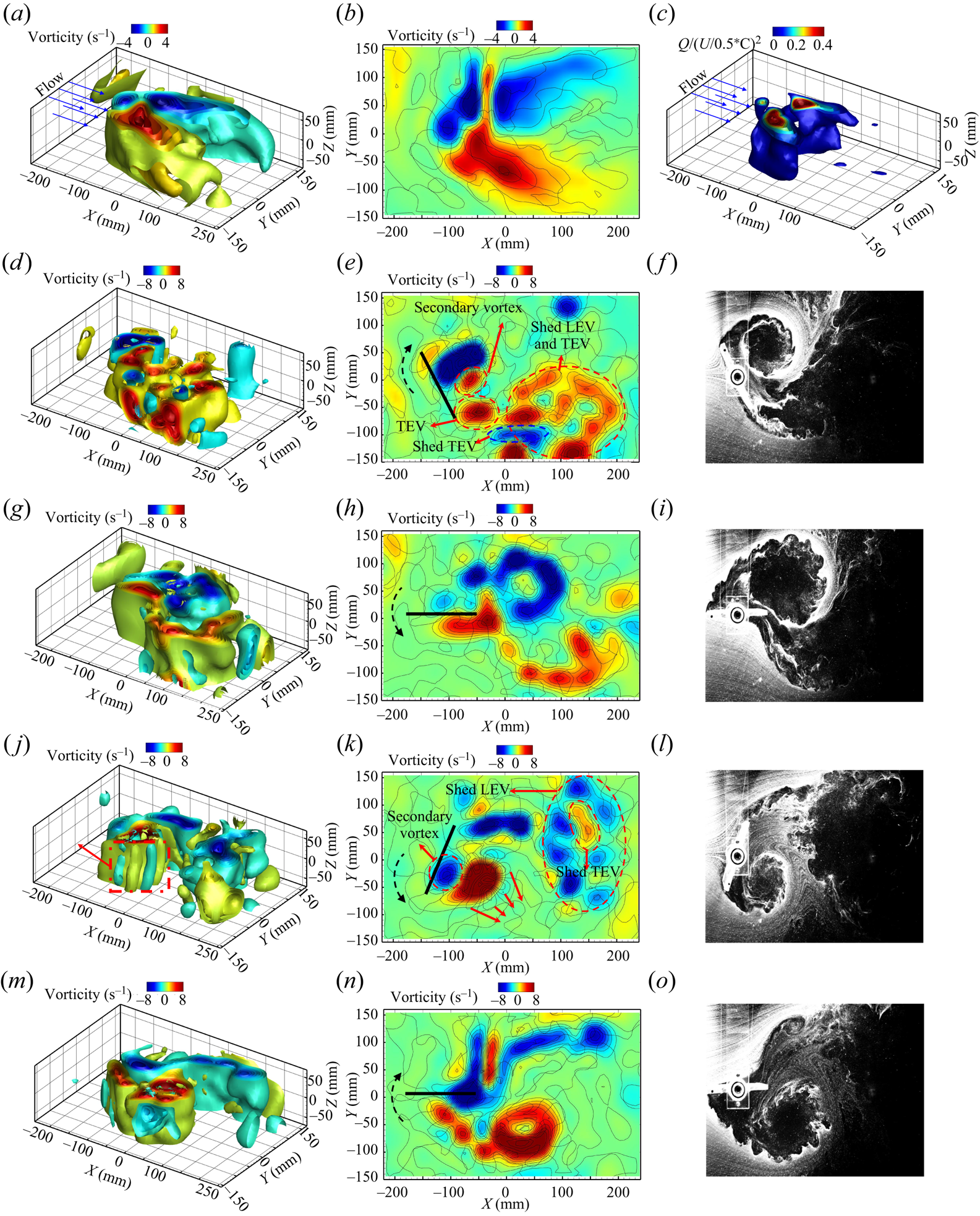
 $Q$-criterion contours and two-dimensional and three-dimensional vorticity. In addition, snapshots of hydrogen bubble flow visualisation were taken at the corresponding phases of the plate (upstroke and downstroke) to gain further insights into the flow evolution and the influence of the free surface. Detailed visualisations can be found in figures 21–23, offering insightful observations on the topic. In general, the formation of a LEV comes from flow separation happening at the sharp leading edge of the plate. This separation creates a low-pressure area at the leading edge, pulling the fluid from the top of the plate down and around the edge (the suction side of the plate). Initially, as the plate starts to show static deflection, a shear layer is created by vorticity at the edge, quickly rolling up into the LEV. As the LEV grows, it forms a region of reversed flow and secondary vorticity forms on the plate's surface under the LEV. When the plate starts oscillating, the shear layer feeds the LEV, causing it to grow in size and strength. After traveling about three chord-lengths, the LEV separates from the plate, shown in figures 21(d–f), and convects into the wake.
Time-averaged three-dimensional vorticity (a,c,e,g) and normalised  $Q$-criterion (b,d,f,g) for the 1DoF system at different reduced velocities: (a,b)
 $U^*=3.01$, (c,d)
 $U^*=3.76$, (e,f)
 $U^*=4.32$ and (g,h)
 $U^*=5.26$, all at
 $H^*=26$.
Time-averaged three- and two-dimensional vorticity field and  $Q$-criterion (a–c), instantaneous three- and two-dimensional vorticity (a,d,g,j,m and b,e,h,k,n) and hydrogen bubble snapshots of the 1DoF system at
 $U^*=4.32$ and
 $H^*=26$.
Time-averaged three- and two-dimensional vorticity field and  $Q$-criterion (a–c), instantaneous three- and two-dimensional vorticity (a,d,g,j,m and b,e,h,k,n) and hydrogen bubble snapshots of the 1DoF system at
 $U^*=4.32$ and
 $H^*=10$.

Time-averaged three- and two-dimensional vorticity field and  $Q$-criterion (a–c), instantaneous three- and two-dimensional vorticity (a,d,g,j,m and b,e,h,k,n) and hydrogen bubble snapshots of the 1DoF system at
 $U^*=4.32$ at
 $H^*=5$.

The first row of figure 21(a–c) shows two symmetric vortices of equal size and strength. This is evident from the analysis of the time-averaged vorticity field and the  $Q$-criterion. The second row of figure 21 shows the growth of negative (clockwise [CW] rotation) LEVs during the upstroke motion and the positive (counterclockwise [CCW] rotation) shed LEV from the previous cycle during the downstroke motion, together with a positive starting vortex at the trailing edge, also known as trailing-edge vortex. These LEVs and TEVs are subsequently convected downstream by the cross-flow and interact with the shed LEV. In the downstroke motion, the fourth row of figure 21(j–l) shows the shedding of positive LEVs of the same size. These symmetric vortex structures of negative and positive LEVs align with the relatively small mean value of oscillation as shown in figure 2(b). In addition, secondary vortices and Kelvin–Helmholtz (K–H) instabilities are observed in both the upstroke and downstroke motions, as shown in figure 21(e,j,k). Shed LEVs and TEVs are visible in the third and fifth rows of figure 21, respectively, representing an almost
 $\theta =0^\circ$ when the plate rotates back from the upstroke and downstroke positions.
In the case of the 1DoF system, as discussed in § 3.1, when the plate is brought closer to the surface, ( $H^*\le 10$), the plate interacts with the free surface. This interaction leads to a shift in the onset of instabilities to higher reduced velocities and a decrease in the oscillation amplitude.
Figure 22(a,b) help us understand the flow dynamics through the time-averaged vorticity field for the plate at the submerged depth of  $H^*=10$. The results show the influence of the plate and free surface on the flow patterns. Notably, this interaction leads to an elongated upstroke LEV compared with the intact LEV observed during the downstroke motion. Figure 22(c) shows the time-averaged
 $Q$-criterion contour, offering further insights into the flow characteristics. It shows a smaller and weaker vortex during the upstroke motion in contrast to the downstroke motion, highlighting the effect of the plate–free surface interaction on the size and strength of the vortices.
During the upstroke motion, shown in figure 22(d–f), the plate, and free surface interaction generate a CCW vortex beneath the free surface. This CCW vortex pairs with the CW growing LEV and interacts with the growing TEV and oblique shed TEV from the previous downstroke motion. The shed upstroke LEV then interacts with the CCW vortex on the free surface and elongates as it is convected downstream by the cross-flow, as shown in figure 22(g–i). Similarly, during the downstroke motion (figure 22j–l), the CW TEV interacts with the free surface and elongates downstream. The hydrogen bubble visualisation and two-dimensional vorticity contour in figure 22(k,l) show that the shed TEV exhibits a distinct downward inclination, resembling an oblique downward jet. This oblique downward jet phenomenon has also been reported in experimental and numerical studies of cylinders in close proximity to the free surface (Sheridan, Lin & Rockwell Reference Sheridan, Lin and Rockwell1997; Carberry, Sheridan & Rockwell Reference Carberry, Sheridan and Rockwell2004; Reichl et al. Reference Reichl, Hourigan and Thompson2005). Figure 22(g,h) show the plate's phase during its downward motion, revealing the presence of paired CCW and CW vortices near the free surface, which are subsequently convected downstream of the plate. Notably, figure 22(h), along with the elongated time-averaged vorticity field displayed in figure 22(a,b), demonstrates that the interaction between the LEV and the free surface leads to the fragmentation of the shed LEV into three smaller CW vortices along the suction side of the plate. In addition, figure 22(i), showcasing a snapshot of the hydrogen bubble, highlights the interaction between the shed LEV and the free surface. As the plate returns from its maximum point in the downstroke motion, the oblique TEV can be observed alongside the intact shed LEV in figure 22(m–o). To summarise, the smaller and elongated LEV during the upstroke motion compared to the downstroke motion, resulting from the fragmentation and pairing of vortices near the free surface, is demonstrated in figure 22. The reduction in oscillation amplitude and the increase in the dominant frequency of oscillation, as discussed in § 3.1.1, can be interpreted as a consequence of the asymmetry shown here in the vortices generated during the upstroke and downstroke motions.
As the plate is placed closer to the free surface ( $H^*=5$), the influence of the free surface on the vortices over and in the wake of the plate becomes more pronounced. This is because the presence of the free surface introduces surface waves and disturbances that interact with the vortices and create pressure gradients, leading to alterations in the flow around the plate and affecting both the vortices and the structural response of the plate.
Figure 23 shows similar plots to figure 22 but for  $H^*=5$. The time-averaged vorticity and
 $Q$-criterion in figure 23(a–c) show significant modifications to the vortices in the vicinity of the free surface, resulting in a non-symmetric LEV during the upstroke and downstroke motions. Figure 23(a,b) show that the time-averaged vortex during the upstroke motion is convected downstream compared with the downstroke undisturbed vortex. In the upstroke motion, when the plate reaches its maximum angle, the LEV is convected downstream and becomes fragmented, as shown in figure 23(d–f). During the downstroke motion, shed LEV and a CCW vortex from the free surface interact with the plate at
 $\theta =0^\circ$, as shown in figure 23(g–i). In addition, a vortex is entrained from the free surface by the plate during the downstroke motion, along with the growing LEV with embedded K–H instabilities, as shown in figure 23(j–l). The interaction between the trailing edge of the plate and the oblique vortices that exhibit a downward orientation almost perpendicular to the plate. The downstream convection of the free surface vortices, paired with the shed TEV from the previous cycle, can be observed in figure 23(m–o). The asymmetry in the vortex structures, characterised by net positive vorticity (CCW vortex), is likely responsible for the net negative lift force exerted on the plate. This observation is supported by the large negative mean oscillation amplitude shown in figure 2(b) and the increase in the dominant frequency of oscillation accompanied by superharmonic frequencies shown in figure 3(d).
3.2.2. Flow analysis for a plate with two DoFs
In this section, we examine the fluid flow behaviour around a plate undergoing 2DoF in both pitching and plunging directions. The investigation involved the analysis of three- and two-dimensional flow using TR-PTV and hydrogen bubble visualisation techniques.
We focused on the analysis of the sample reduced velocity of  $U^*=4.32$ at different submerged heights:
 $H^*=26$,
 $H^*=10$ and
 $H^*=5$. Figures 24–26 present the time-averaged vorticity,
 $Q$-criterion contours, two- and three-dimensional instantaneous vorticity, as well as hydrogen bubble flow visualisation snapshots of one full cycle of oscillation, respectively. When the plate is allowed to oscillate in both pitching and plunging modes, the plunging oscillation causes the TEV to roll up on the suction side of the plate shown in figure 24(e,f). These vortices grow in size compared with the 1DoF system. In addition, due to the increased interaction between the plate and the cross-flow, the wake of the plate in the 2DoF system contains more small vortices compared with the 1DoF system. Figure 24(d,e) highlights the presence of a noisier wake compared with the 1DoF system (figure 21), with numerous small vortices caused by the intense interaction of shed TEVs and LEVs with the wake vortices.
Time-averaged three- and two-dimensional vorticity field and  $Q$-criterion (a–c), instantaneous three- and two-dimensional vorticity (a,d,g,j,m and b,e,h,k,n) and hydrogen bubble snapshots of the 2DoF system at
 $U^*=4.32$ at
 $H^*=26$.

Time-averaged three- and two-dimensional vorticity field and  $Q$-criterion (a–c), instantaneous three- and two-dimensional vorticity (a,d,g,j,m and b,e,h,k,n) and hydrogen bubble snapshots of the 2DoF system at
 $U^*=4.32$ at
 $H^*=10$.

Time-averaged three- and two-dimensional vorticity field and  $Q$-criterion (a–c), instantaneous three- and two-dimensional vorticity (a,d,g,j,m and b,e,h,k,n) and hydrogen bubble snapshots of the 2DoF system at
 $U^*=4.32$ at
 $H^*=5$.
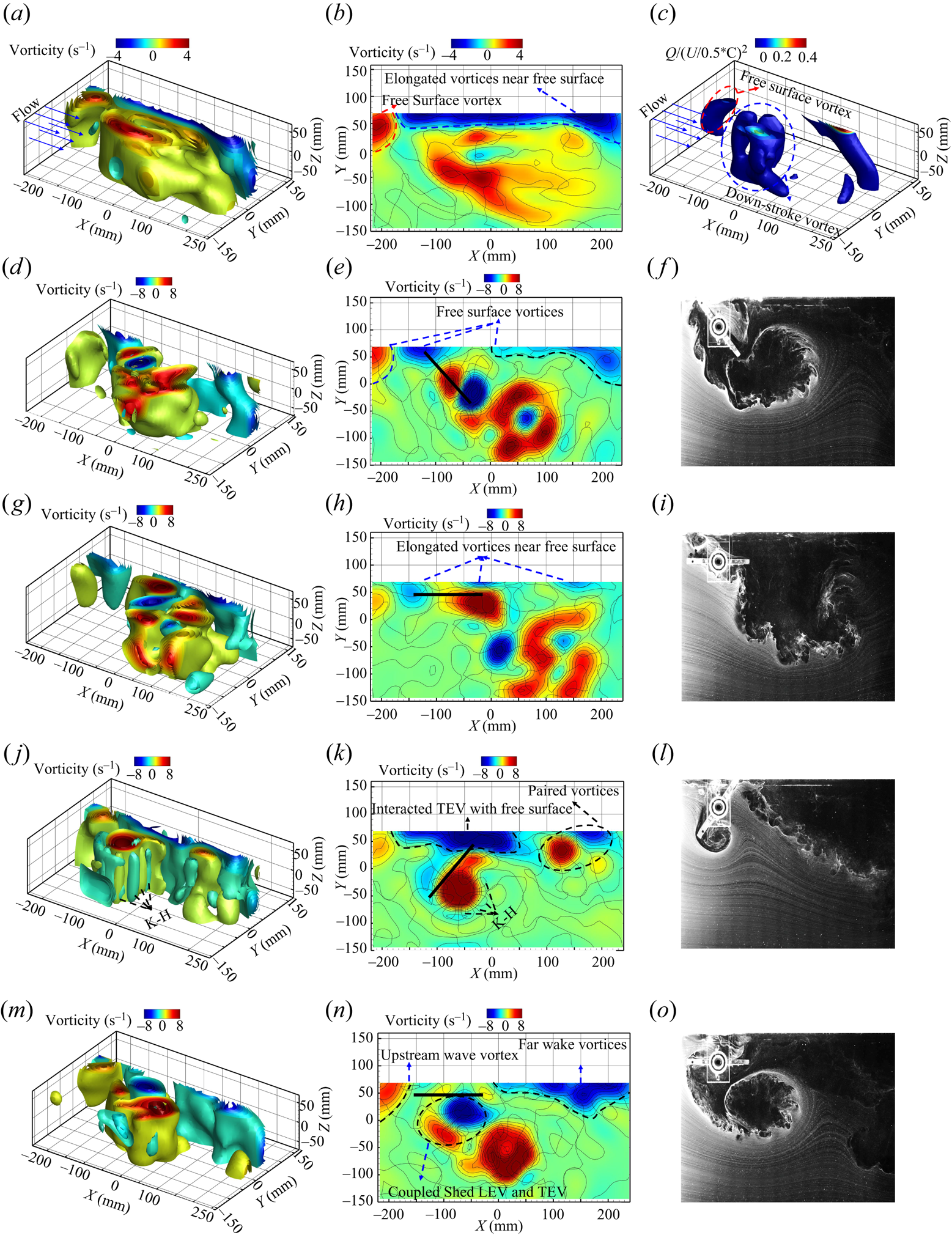
Similar to the 1DoF system shown in figures 22 and 23, as the submerged heights decrease, there is an interaction between the shed LEVs and TEVs with the free surface during both the upstroke and downstroke motions. However, in the case of the 2DoF system, where both pitching and plunging motions are involved, the plate is brought closer to the free surface compared to a pure pitching mode (1DoF). This proximity results in a greater interaction between the plate and the free surface.
Figure 25 shows the time-averaged vorticity and  $Q$-criterion for a submerged height of
 $H^*=10$. In the time-averaged vorticity vector field (figure 25a,b), a higher number of vorticity cores are observed during the upstroke motion, indicating an increased interaction between the 2DoF plate and the free surface. This interaction leads to a more elongated and fragmented vorticity structure near the free surface compared with the 1DoF system (figure 22a,b). In addition, the shed vortices during the downstroke motion exhibit greater size and strength in comparison with the pure pitching mode (figure 22b). The inclined shed TEV is observed during the upstroke motion (figure 25e), aligning closely with the downward angle of the plate.
In this work, we qualitatively observed the deformation of the free surface induced by the plate's proximity. This proximity led to the generation of surface waves both upstream and downstream of the plate. Although our current experimental set-up does not facilitate a detailed and quantitative analysis of these surface deformations, our primary focus is on investigating the dynamic flow patterns. The surface deformations and resulting waves are presumed to be responsible for the formation of vortices beneath the free surface, a phenomenon quantified in our study, revealing the complex dynamics of the system involving the plate, the free surface and the flow. Notably, we recognise a likely correlation between the observed vortex dynamics and the qualitative surface deformation. Figure 25(d–f) shows the interplay between the shed vortices and the qualitatively noted free surface deformation. The formation of counter-rotating vortices in the far-wake region, positioned between the shed vortices and surface wave vortices near the free surface, suggests a compelling association with the qualitatively observed surface deformation.
As the plate is brought even closer to the free surface, the interaction between the plate and the free surface becomes significantly stronger. Figure 26 shows similar plots to figure 25 but for  $H^*=5$ for the 2DoF system. The time-averaged vorticity field in figure 26(a,b) reveals that the vorticity near the free surface becomes highly elongated and continues downstream of the plate. This contrasts the nearly dissipated vorticity observed in the 1DoF system (figure 23a,b) which highlighting increased interaction between the deformed free surface, corresponding surface waves and vortices, with the plate and shed LEVs and TEVs. The time-averaged
 $Q$-criterion (figure 26c) shows the presence of the downstroke vorticity core and a small contribution of upstream and downstream vorticity near the free surface. The instantaneous vector fields in figure 26(d–o) show various flow phenomena, including the generation of upstream vortices through the coupling and pairing of vortices near the free surface and the near-field wake, K–H instabilities, the interaction between shed LEVs and TEVs, and the formation of vortices in the far-wake region. It is noteworthy that these near-surface vortices (shown in figures 25 and 26), such as coupled and surface wave vorticity, appear in the time-averaged measurements because they persist throughout the plate's oscillation and are strong enough to survive the averaging process. These vortices can be associated with the presence of superharmonic frequencies and the reduction in the amplitude of the structural response, as discussed and demonstrated in figure 7 and 9.
3.2.3. Analysis using POD
This section focuses on the application of the POD method to analyse the flow visualisation results and understand the influence of coherent structures, particularly shed vortices along the flat plate affected by the free surface. The POD method, a modal decomposition technique, enables the extraction of dominant modes of variation by reducing the dimensionality of large data sets. It was initially proposed by Lumley (Reference Lumley2007) to identify coherent structures in turbulent flows and has since become a widely used approach to investigate flow dynamics (Berkooz, Holmes & Lumley Reference Berkooz, Holmes and Lumley1993; Sieber, Paschereit & Oberleithner Reference Sieber, Paschereit and Oberleithner2016; Taira et al. Reference Taira, Brunton, Dawson, Rowley, Colonius, McKeon, Schmidt, Gordeyev, Theofilis and Ukeiley2017). By employing singular value decomposition (SVD) on the data matrix, the POD method generates a set of orthogonal basis vectors and singular values. These basis vectors represent the most energetic structure in the data. The leading basis vectors, associated with the largest singular values, capture the majority of the data's fluctuations and allow for the reconstruction of the original data with minimal information loss. Therefore, POD can effectively reduce the dimensionality of the data by projecting it onto the subspace spanned by the dominant basis vectors.
To apply POD, the unsteady flow field, denoted as  $u$, is decomposed using the Reynolds decomposition approach into a time-averaged flow field,
 $\bar {U}$, and fluctuating flow,
 $u^\prime$, as (Taira et al. Reference Taira, Brunton, Dawson, Rowley, Colonius, McKeon, Schmidt, Gordeyev, Theofilis and Ukeiley2017)
 \begin{equation} u=\bar{U}+u^\prime. \end{equation}
In this study, the snapshot POD method, originally proposed by Sirovich (Reference Sirovich1987), is employed to analyse the fluctuation of a vector field by linearly combining orthonormal modes obtained from solving an eigenvalue problem. Following the approach described in Meyer, Peder & Özcan (Reference Meyer, Peder and Özcan2007), the POD modes are calculated based on the velocity fluctuations. However, it has been shown that using the vorticity vector field yields comparable results (Ma, Karamanos & Karniadakis Reference Ma, Karamanos and Karniadakis2000).
In the snapshots approach, the spatiotemporal fluctuation velocity field, denoted as  $u_i^\prime (x,t)$, can be decomposed into two components: one related to the unsteady spatial basis functions
 $\phi _k(x)$ and their corresponding temporal characteristics
 $a_k(t)$, as expressed by the equation
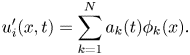 \begin{equation} u_i^\prime(x,t) = \sum_{k=1}^{N} a_k(t)\phi_k(x). \end{equation}
Here,  $k$ can take value from 1 to
 $N$, where
 $N$ represents the number of snapshots used in the calculation and
 $i$ shows the dimensions of the velocity field. This equation represents the fluctuation flow field using a set of basis functions
 $\phi _k$, which form an orthonormal basis. SVD is applied to the obtained three-dimensional fluctuation velocity field
 $(u-\bar {U})$ to calculate the spatial modes (
 $\phi _k(x)$) and their corresponding temporal modes (
 $a_k(t)$) (Saad Reference Saad2011), given by
 \begin{equation} (\phi, \sqrt{\lambda}, a) = svd(u-\bar{U}). \end{equation}
In the above equation, the eigenvalues  $\lambda$ represent the energy collected from the POD modes
 $\phi (x)$. The resulting eigenvalues
 $\lambda$ are arranged in descending order to ensure that the energy-intensive modes are prioritised. The zeroth mode corresponds to the time-averaged flow field, with a temporal coefficient of one, which is subsequently removed from the flow field for further analysis.
Figure 27 presents the energy distribution of the first 60 POD modes as a percentage of the total energy at three submerged heights,  $H^*=26$,
 $H^*=10$ and
 $H^*=5$, for both the 1DoF and 2DoF systems at a sample reduced velocity of
 $U^*=4.32$, which was previously discussed in terms of the structural response and flow visualisations. It can be observed that the higher POD modes beyond the fourth mode contain less than
 $5\,\%$ of the total energy. However, as explained in the upcoming section, these modes still possess significant spatial structures that represent coherent patterns, and their temporal coefficients exhibit a coherent temporal pattern over time. Although these higher modes have a lower energy content, indicating their minor contribution to the overall flow field, they capture smaller and less-prominent structures. In this study, our focus is on investigating the first eight POD modes, which is discussed in detail in the following section.
Energy distribution for the first 60 POD modes of (a) the 1DoF system and (b) the 2DoF system at  $U^*=4.32$ for three submerged heights:
 $H^*=26$,
 $H^*=10$ and
 $H^*=5$.
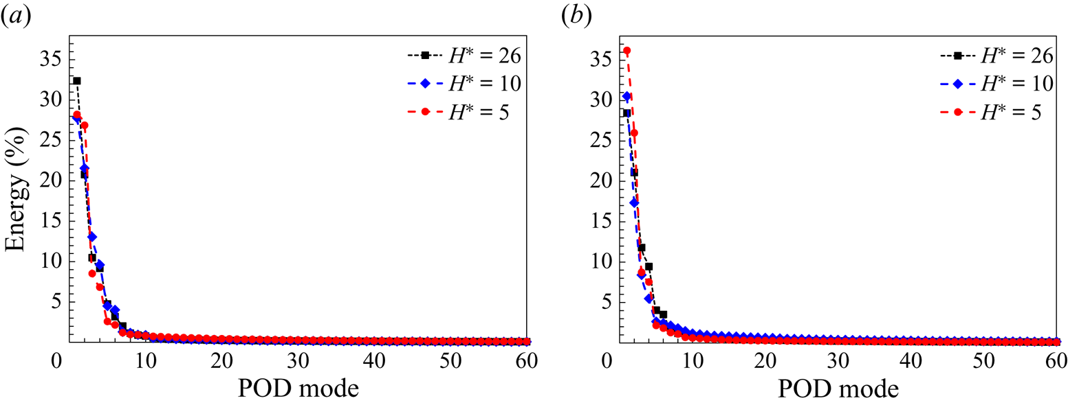
Figure 28 shows the three-dimensional spatial structure of the first eight POD modes, represented by the vorticity field, for the 1DoF system. The modes are shown for three submerged heights,  $H^*=26$,
 $H^*=10$ and
 $H^*=5$, at a sample reduced velocity of
 $U^*=4.32$. The figures labelled as (a i–a viii), (b i–b viii) and (c i–c viii) correspond to the modes for each respective submerged height. Figures 29–31 present additional information about the temporal behaviour of the POD modes. In the first row of these figures, phase plots of consecutive temporal modes are displayed. The second row shows the time evolution of the first eight POD temporal coefficients, along with their corresponding frequency contents. The third row presents phase portraits of the first POD mode plotted against the higher POD modes for each of the three submerged heights.
Spatial structure of the vorticity vector field for the first eight POD modes of the 1DoF system at  $U^*=4.32$ for three submerged heights: (a i–a viii)
 $H^*=26$, (b i–b viii)
 $H^*=10$ and (c i–c viii)
 $H^*=5$.
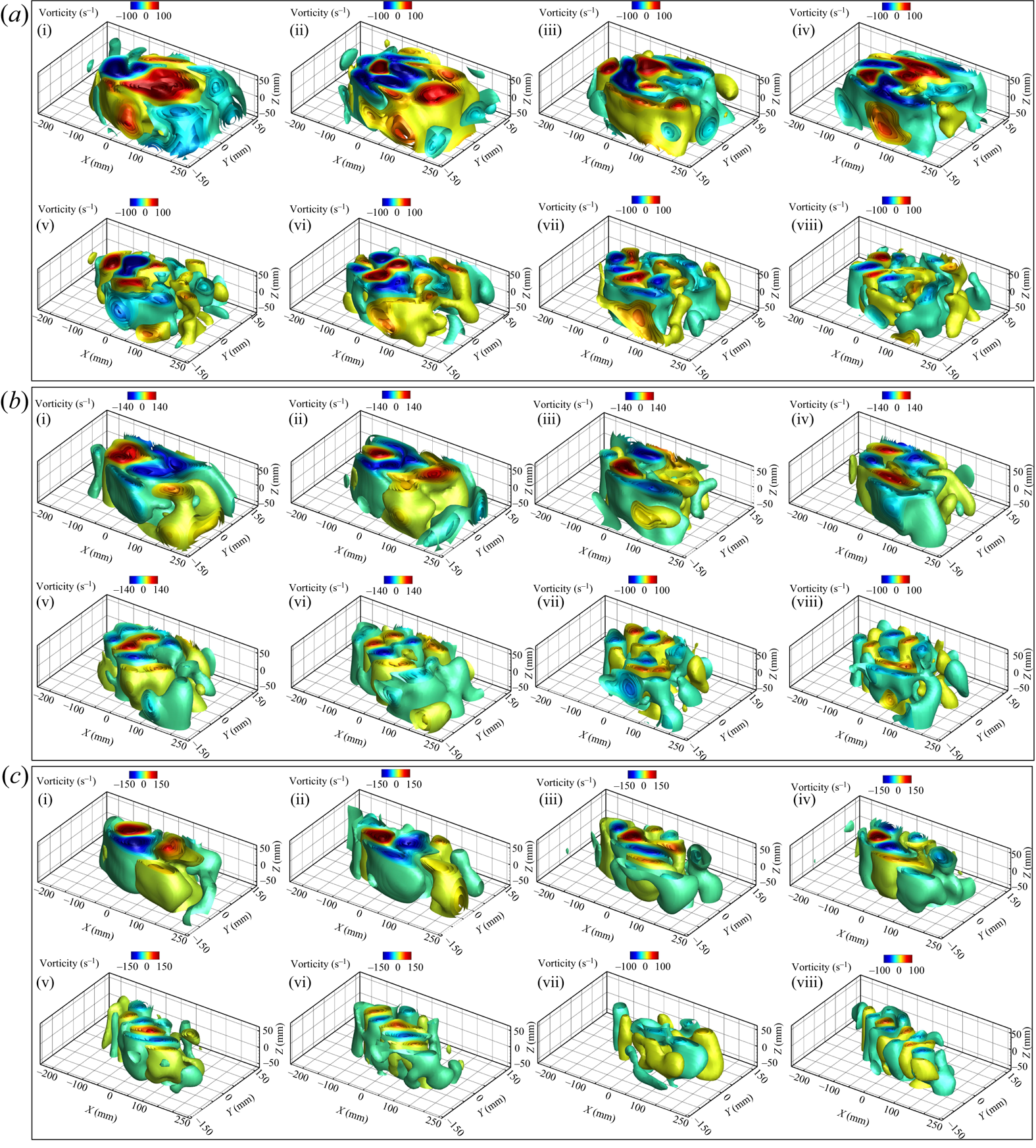
Phase portraits of temporal modes (a i–a iv), time evolution of the first eight temporal coefficients with their corresponding frequency contents (FFT plots) (b i–b iv) and phase portraits of  $a_1$ vs higher POD modes (c i–c iii) of the 1DoF system at
 $U^*=4.32$ for
 $H^*=26$.

Phase portraits of temporal modes (a i–a iv), time evolution of the first eight temporal coefficients with their corresponding frequency contents (FFT plots) (b i–b iv) and phase portraits of  $a_1$ vs higher POD modes (c i–c iii) of the 1DoF system at
 $U^*=4.32$ for
 $H^*=10$.

Phase portraits of temporal modes (a i–a iv), time evolution of the first eight temporal coefficients with their corresponding frequency contents (FFT plots) (b i–b iv) and phase portraits of  $a_1$ vs higher POD modes (c i–c iii) of the 1DoF system at
 $U^*=4.32$ for
 $H^*=5$.

Based on the spatial structure, the POD modes can be divided into two groups:  $A_1$ and
 $A_{-1}$. The
 $A_1$ group consists of modes 1, 2, 5 and 6, which exhibit a symmetric spatial structure. The
 $A_{-1}$ group includes the mean flow and modes 3, 4, 7 and 8, which display an antisymmetric structure. These spatial modes capture the dominant coherent structures associated with the shedding of LEVs and TEVs during the upstroke and downstroke motion. Previous studies, such as Konstantinidis, Balabani & Yianneskis (Reference Konstantinidis, Balabani and Yianneskis2007), have noted that the antisymmetric vorticity field is represented by the symmetric spatial structure of the POD vorticity field, and vice versa. Therefore, the first and second POD modes are believed to represent the dominant coherent structures related to the shed LEVs and TEVs during the plate's oscillation, whereas the higher POD modes reveal more intricate coherent structures, including secondary vortices and interacting vortices observed over and within the wake of the plate.
The periodic motion of the plate during oscillation, whether in a 1DoF or 2DoF system, leads to a periodic flow across the plate. This periodic flow allows for the formation of paired mode patterns in the flow field. Paired modes are characterised by similar spatial structures and a  ${\rm \pi} /2$ radian phase shift in the distribution of their temporal coefficients. These characteristics can be represented by circular shapes in the amplitude correlation between the temporal coefficients of the POD modes.
For  $H^*=26$, the POD modes 1 and 2, 3 and 4, 5 and 6, and 7 and 8 exhibit similar vortical structures. This visual similarity is evident in figure 29(a i–a iv), where the phase portraits display circular shapes with a
 ${\rm \pi} /2$ phase difference. The frequency contents of the temporal coefficients for (
 $a_1$ and
 $a_2$), (
 $a_3$ and
 $a_4$), (
 $a_5$ and
 $a_6$) and (
 $a_7$ and
 $a_8$) align closely, indicating synchronised oscillatory behaviour. Thus, these modes can be considered as paired modes. The dominant frequency observed in the first and second POD modes, as shown in figure 29(b i), is similar to the frequency observed in the structural response of the system (figure 4c i). The pairs (
 $a_1$ and
 $a_2$), (
 $a_3$ and
 $a_4$), (
 $a_5$ and
 $a_6$) and (
 $a_7$ and
 $a_8$) have frequencies of
 $f^*_1$,
 $2f^*_1$,
 $3f^*_1$ and
 $4f^*_1$, respectively. This indicates that the frequencies of the temporal coefficients in groups
 $A_1$ and
 $A_{-1}$ are odd and even multiples of the dominant frequency
 $f^*_1$.
Figures 29(a i) and 29(c i–c iii) show the phase portraits of the higher temporal POD modes with respect to the first mode. These phase portraits show trajectories in the shape of circles, lemniscates (or infinity signs) and interlocked loops. They highlight the odd and even multiples of the dominant frequency  $f^*_1$ and demonstrate the harmonic nature of the temporal coefficients, as well as the phase differences between the temporal coefficients. Therefore, the different signs of spatial structure, symmetric and antisymmetric, can be attributed to the frequency characteristics of the temporal coefficients of
 $A_1$ and
 $A_{-1}$.
As discussed in the previous section (§ 3.2.1), the vortical structure of the plate undergoing LCO is significantly influenced when the plate approaches the free surface. Figure 28(b i–b viii) presents the spatial structure of the POD modes at  $H^*=10$ and
 $U^*=4.32$. As observed in figure 22, the interaction between the shed vortices and the free surface leads to the fragmentation of vortices, as seen in the instantaneous vorticity contours and hydrogen bubble visualisation. This breakup is also evident in the time-averaged vorticity contours (figure 22a–c), where the symmetric structure of the two vortex tubes is disrupted. A similar observation can be made from the spatial structure of the POD modes shown in figure 28(b i–b viii), where the vortical structures of the shed vortices during the downstroke motion appear larger than those during the upstroke motion (figure 22a,d,j). Nevertheless, symmetric and antisymmetric spatial structures are still observed in the groups
 $A_1$ and
 $A_{-1}$.
The structural response of the 1DoF system, as shown in figure 5, reveals the presence of superharmonic frequency contents as the plate approaches the free surface. Moreover, these superharmonic frequency contents are also observed in the higher POD modes, specifically in modes (3 and 4) and (7 and 8), as shown in figure 30(b ii,b iv). The phase portrait of  $a_3$ and
 $a_4$ shown in figure 30(a ii) shows two distinct closed loops with different amplitudes, indicating the presence of superharmonic frequency content in the temporal coefficients.
When the plate is brought closer to the free surface at  $H^*=5$, the influence of the free surface on the shed vortices becomes even more pronounced, as shown in figure 23. Figure 28(c i–c viii) shows the spatial structure of the POD modes for
 $H^*=5$ at
 $U^*=4.32$. Notably, oblique downward vortical structures are observed in the POD spatial patterns emphasising the negative mean oscillation amplitude observed in figure 2(b). The presence of paired POD modes is confirmed by the phase portraits of the temporal coefficients shown in figure 31. However, the phase portrait of temporal coefficient of
 $a_7$ and
 $a_8$ exhibits scattered and irregular patterns, reflecting the non-harmonic time history of
 $a_7$ shown in figure 31(c iv). Consequently, reducing
 $H^*$ to 5 for the 1DoF system results in the degradation of these two higher POD modes. In addition, the strength of the vortical structures in modes 5 to 8 decreases compared with the higher submerged depth, indicating the dissipation of vortices due to the influence of the free surface.
Figures 32–37 present similar plots to figures 28–31, but for the 2DoF system. In the 2DoF system, as in the 1DoF system, the spatial structures obtained through POD can be categorised into symmetric ( $A_1= 1, 2, 5\mbox { and 6}$) and antisymmetric (
 $A_{-1}={\text {mean flow}, 3, 4, 7\text { and }8}$) patterns, as observed in figure 32. Moreover, the spatial structures and phase portraits of consecutive temporal modes show the presence of paired modes in the 2DoF system as well.
Spatial structure of the vorticity vector field for the first eight POD modes of the 2DoF system at  $U^*=4.32$ for three submerged heights: (a i–a viii)
 $H^*=26$, (b i–b viii)
 $H^*=10$ and (c i–c viii)
 $H^*=5$.
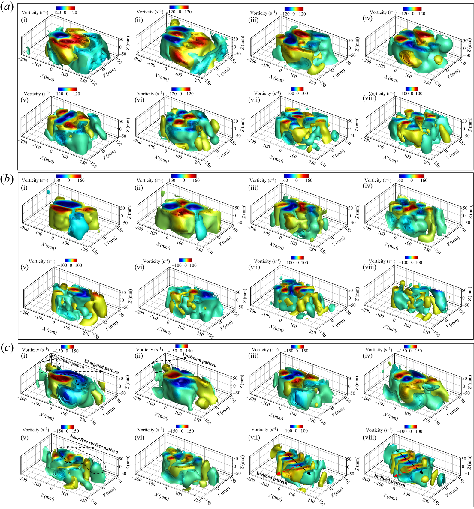
Phase portraits of temporal modes (a i–a iv), time evolution of the first eight temporal coefficients with their corresponding frequency contents (FFT plots) (b i–b iv) and phase portraits of  $a_1$ vs higher POD modes (c i–c iii) of the 2DoF system at
 $U^*=4.32$ for
 $H^*=26$.

Phase portraits of temporal modes (a i–a iv), time evolution of the first eight temporal coefficients with their corresponding frequency contents (FFT plots) (b i–b iv) and phase portraits of  $a_1$ vs higher POD modes (c i–c iii) of the 2DoF system at
 $U^*=4.32$ for
 $H^*=10$.
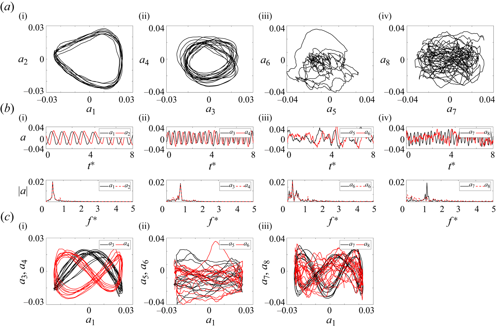
Spatial structure of the vorticity vector field for first eight POD modes of the 2DoF system at  $U^*=4.70$ for three submerged height
 $H^*=10$.

Phase portraits of temporal modes (a i–a iv), time evolution of the first eight temporal coefficients with their corresponding frequency contents (FFT plots) (b i–b iv) and phase portraits of  $a_1$ vs higher POD modes (c i–c iii) of the 2DoF system at
 $U^*=4.70$ for
 $H^*=10$.

Phase portraits of temporal modes (a i–a iv), time evolution of the first eight temporal coefficients with their corresponding frequency contents (FFT plots) (b i–b iv) and phase portraits of  $a_1$ vs higher POD modes (c i–c iii) of the 2DoF system at
 $U^*=4.32$ for
 $H^*=5$.

The dominant frequency of  $f^*_1$ observed in the first pair of (
 $a_1$ and
 $a_2$) is multiplied by odd and even integers in the higher POD modes of (
 $a_3$ and
 $a_4$), (
 $a_5$ and
 $a_6$) and (
 $a_7$ and
 $a_8$). The phase portraits of the higher temporal POD modes with respect to the first mode of the 2DoF system show trajectories of circular, lemniscate (or infinity sign) and infinity with triple and four interlocked loops, similar to the 1DoF system.
The superharmonic frequencies observed in the structural response of the 2DoF system in figures 12 and 11 are also observed in the higher temporal POD modes of ( $a_5$ and
 $a_6$) and (
 $a_7$ and
 $a_8$) shown in figure 33(c iii,c iv). At
 $H^*=10$, the onset of instabilities is shifted to higher reduced velocities, as discussed in § 3.1. Hence, LCO starts only at this particular sample reduced velocity (
 $U^*=4.32$) for this submerged height in which the higher POD modes (modes 5–8) exhibit small-scale turbulent vortical structures. Therefore, the POD results of another sample of reduced velocity of
 $U^*=4.70$ were shown in figures 36 and 35 to indicate the coherent structure and corresponding superharmonic frequencies which are consistent with the structural results discussed in figures 15 and 16. The higher POD modes of the 2DoF system, unlike the 1DoF system at
 $H^*=5$, exhibit significant coherent spatial structures. This observation is reinforced by the analysis of time evaluation of the frequency content, and the identification of paired modes in the phase portraits shown in figure 37. Notably, these spatial modes display an inclined vortical pattern, an elongated structure, and the presence of vorticity near the free surface shown in figure 35. These characteristics suggest a strong coupling between shed vorticity and the free surface, as well as the existence of surface wave vorticity at a submerged height of
 $H^*=5$. These findings align with the previous discussion and are consistent with the observations in figure 25.
In summary, the analysis of POD modes and flow characteristics in both 1DoF and 2DoF systems has provided valuable insights into the vortical structures and their interactions with the free surface. The POD results have revealed distinct spatial patterns, temporal behaviours and frequency content of the coherent structures present in the flow field. The presence of paired modes, as identified through phase portraits and frequency analysis, highlights the periodic nature and harmonics of the flow. Furthermore, the influence of the free surface on the shed vortices is evident in the POD modes, with the vortical structures exhibiting variations in size, shape and vorticity distribution near the free surface. These findings contribute to a deeper understanding of the complex dynamics of the fluid–structure interaction and the role played by coherent structures in shaping the flow characteristics.
4. Conclusion
In this experimental study, the dynamic response of a flexibly-mounted rigid flat plate, oscillating freely in both pitching and plunging directions, has been investigated. The study has focused on the influence of submerged heights ( $H^*=1-26$) on the plate's behaviour, including oscillation amplitudes and wake structures. Experiments have been conducted across a range of reduced velocities
 $U^*=0.29\unicode{x2013}8.73$, corresponding to Reynolds numbers
 $Re=218\unicode{x2013}15{\,}331$.
The study aimed to understand the onset of instability, analyse fluid–structure–surface interactions response, and examine vortex dynamics in the plate's wake. For a deeply submerged plate with 1DoF in pitching direction, divergence instabilities were observed at the first critical flow velocity, with increasing reduced velocity causing amplitude amplification. Beyond a critical reduced velocity, the plate underwent periodic LCOs, with increasing amplitudes up to a third critical reduced velocity where LCOs were fully suppressed. Higher flow velocities led to divergence instability and an increase in the static divergence angle of the plate.
The fluid–structure–surface interaction response of the system was significantly influenced by the submerged height. For  $H^*\geq 15$, the overall fluid–structure–surface interactions response in the 1DoF system was consistent. However, reducing
 $H^*$ shifted the onset of instabilities to higher reduced velocities, decreased amplitude, width, the mean value of oscillation, and occurrence of the second range of divergence instability. Oscillations initiated with higher-frequency content compared with
 $H^*\geq 15$. Superharmonic frequencies were detected near the free surface in the 1DoF system. Static divergence instabilities were encountered at all tested reduced velocities for
 $H^*\leq 2.5$ and
 $H^*\leq 1$.
For the 2DoF system, synchronisation of pitching and plunging oscillation frequencies was observed for the tested submerged heights. Increasing reduced velocity revealed the contribution of superharmonic frequencies. Broad-banded frequency response in both modes was observed at high reduced velocities. Similar to the 1DoF system, oscillations in pitching and plunging directions initiated with higher frequency content compared to  $H^*\geq 15$. Decreasing submerged height below
 $H^*\leq 10$ significantly enhanced the influence of the free surface. The range of LCOs expanded, with an increase in plunging amplitude despite a decrease in pitching amplitude. The onset of oscillation and the second range of static divergence occurred at higher reduced velocities. The widest oscillation region was observed for the 2DoF system at
 $H^*=5$. Oscillations were minimal for
 $H^*=2.5$. In addition, the FIV response of the 2DoF system exhibited non-periodic oscillations with larger amplitude at high reduced velocities and lower submerged height.
To investigate vortex dynamics, qualitative and quantitative flow visualisation techniques were employed. Hydrogen bubble visualisation provided insights into overall flow behaviour, whereas TR-PTV allowed for detailed analysis of flow field dynamics at different reduced velocities. In the deeply submerged case, symmetric shedding LEV and TEV indicated negligible free surface influence on plate response in both 1DoF and 2DoF systems. Decreasing submerged height intensified the interaction between shed vortices and the free surface, resulting in the breakdown of the symmetric wake. Elongated and fragmented vortices near the free surface were observed for  $H^*\leq 10$, influenced by surface waves and coupled with shed vortices downstream of the plate.
The POD technique has been employed to analyse the spatiotemporal characteristics of coherent structures. Based on energy levels, temporal coefficients and spatial structures, symmetric and antisymmetric patterns have been identified. Analysis of temporal POD coefficients demonstrated synchronisation of dominant shed vortex frequencies with plate's oscillation. The first eight modes displayed significant and coupled coherent structures, including interaction with the free surface, surface wave vortices and an oblique downward structure in the plate's wake. Temporal POD mode analysis revealed the presence of superharmonic frequencies associated with the plate's oscillation.
This comprehensive investigation of vortex dynamics, combined with the application of the POD technique, has provided valuable insights into the complex flow phenomena surrounding the oscillating plate. The observed coherent structures, their spatial and temporal characteristics, and the identification of superharmonic frequencies contribute to a deeper understanding of the fluid–structure–surface interactions response of the system.
Funding
We gratefully acknowledge the support provided by the National Science Foundation (NSF) through the CAREER CBET program under grant number 2143263.
Declaration of interests
The authors report no conflict of interest.



