Introduction
Bayesian decision theory (BDT; Blackwell & Girshick, Reference Blackwell and Girshick1954) is a mathematical theory of decision making based on game theory (von Neumann & Morgenstern, Reference von Neumann and Morgenstern1944/1953) that has proven to be a powerful tool in mathematical statistics (Ferguson, Reference Ferguson1967; Berger, Reference Berger1985; O’Hagan, Reference O’Hagan1994; Gelman et al., Reference Gelman, Carlin, Stern and Rubin2003; Jaynes, Reference Jaynes2003). It also serves as a useful framework for developing models of biological perceptual processing (Knill & Richards, Reference Knill and Richards1996; Maloney, Reference Maloney, Heyer and Mausfeld2002; Mamassian et al., Reference Mamassian, Landy, Maloney, Rao, Lewicki and Olshausen2002), in part because its mathematical structure is evocative of the ordinary “perceptual cycle” (Neisser, Reference Neisser1976).
The elements of BDT
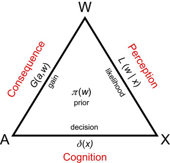
The elements of BDT are summarized in Fig. 1 as three sets and four functions. The three sets are W, the states of the world; X, possible sensory states; and A, possible actions. On every “turn,” the world is in some specific state,  , unknown to the organism. The organism is given access to a sensory state,
 , and must decide what action,
 , to select.
(Color online) The elements of BDT. The three vertices correspond to W, the possible states of the world; X, the possible sensory states; and A, the available actions. The three edges correspond to the gain function G(a,w), the likelihood function  , and the decision rule δ(x), where
 denotes a sensory state,
 a particular action, and
 a particular state of the world. The last element is the prior distribution π(w) on the possible states of the world.

There are four functions that serve to complete the description of the BDT task. Typically, the first is the prior π(w), the probability densityFootnote 1 that any particular state of the world is the current state. The second is the likelihood function  , the probability density of sensory states which as written depends on the state of the world. This function is typically written as
 to emphasize that it provides information about possible states of the world given a particular sensory state x. Remarkably, it can be shown that the likelihood function captures all of the sensory information relevant to the state of the world (Berger & Wolpert, Reference Berger and Wolpert1988; Maloney, Reference Maloney, Heyer and Mausfeld2002), a result known as the likelihood principle.
The third function is the gain function G(a,w) that determines the gain or loss experienced by the organism on a particular trial. It is also referred to as loss function or value function in the literature. We use the term gain function with the understanding that losses are coded as negative gains. The last function is the decision function a = δ(x) that captures the strategy of a particular BDT observer. Given a sensory state (the only novel information available on a particular trial), the observer selects an action. Each possible decision function corresponds to a different possible observer.
The Bayes observer, by definition, selects the action that maximizes expected gain on any turn by choice of the decision rule:

If it is not plausible that the organism has access to the prior in a particular task, then BDT becomes statistical decision theory (Maloney, Reference Maloney, Heyer and Mausfeld2002), and it is still possible to develop criteria for selection of “good” actions. Here we confine attention to BDT.
In any application of BDT, the elements of BDT play roles that are fairly obvious. The prior captures the statistical structure of the environment, the likelihood function characterizes the instantaneous sensory information that is available, and the gain function specifies the task at hand. The gain function, in particular, represents the consequences to the organism of its actions, and there are as many gain functions as there are natural tasks we might ask an organism to undertake. In an experimental context, the gain function is imposed by the experimenter, and in natural contexts, it is imposed by the environment. The gain function links the organism to objective possibilities of reward and punishment in any particular context. It is typically not under the control of the organism.
One way to organize the Bayesian computation in eqn. (1) is to first multiply prior and likelihood function to form a posterior distribution that summarizes all the information available about the likely distribution of the state of the world but which lacks any information about possible costs and benefits associated with specific actions (the gain function). As we present BDT, we assume that selection of action depends on both this posterior and the gain function. The information in this posterior is a summary of the available information about the state of the world but divorced from the demands of any specific task. Maloney (Reference Maloney, Heyer and Mausfeld2002) speculated that the visual representation of the scene could be identified with this posterior but provided no clear way to test such a claim. The claim that there is a separate visual representation is an intriguing one, but a skeptic might argue that such a claim has no evident consequences for behavior and therefore is not empirically testable. We will not consider this issue further.
Operationalizing perception as Bayesian inference
It is not obvious that any biological organism can solve eqn. (1) and compute δ(x). Researchers have argued that biological organisms are unable to compute eqn. (1) because of its computational complexity and the knowledge presupposed (Shimojo & Nakayama, Reference Shimojo and Nakayama1992).
However, applications of BDT in specific tasks can be rather modest, and part of the opposition to BDT as a process model of human visuomotor performance is typically terminological. In particular applications of BDT, rather grandiose terms such as “states of the world” can simply comprise the location in depth of a visual target or just the presence or absence of such a target. In particular applications of BDT, we will find that the solution is sometimes very simple. Signal detection theory (Green & Swets, Reference Green and Swets1966/1974) and its generalizations (Duda et al., Reference Duda, Hart and Stork2000, Chapter 2) are applications of BDT (Maloney, Reference Maloney, Heyer and Mausfeld2002) with remarkably simple solutions. See Maloney (Reference Maloney, Heyer and Mausfeld2002) for a discussion of the complexity of Bayesian computation.
The terminology of BDT can be misleading in another sense. Researchers familiar with the term prior, for example, may come to think of it as a probability density function applied to events outside the observer or that actions are simple binary decisions or at most univariate estimates of depth, curvature, and so forth. We will describe applications where a single action corresponds to selection of motor plans of great complexity in neural terms and where the prior uncertainty encodes the unavoidable uncertainty in the outcome of speeded movements as well as perceptual uncertainty (Trommershäuser et al., Reference Trommershäuser, Maloney and Landy2008). While the sources of motor uncertainty are endogenous, this uncertainty is beyond the control of the organism and is better modeled as part of the states of the world.
The simplicity of the ideas underlying BDT does not imply that the theory is only appropriate for trivial tasks. Conversely, the apparent complexity of eqn. (1) need not exceed the computational capacities of biological organisms.
Eqn. (1) specifies an ideal observer or actor where the sense in which the observer is optimal is well defined: this Bayes’ observer maximizes expected gain for whatever gain function is specified. We can use eqn. (1) to determine the optimal performance in specific tasks and then compare human performance to this benchmark. Geisler (Reference Geisler1989, p. 30) proposed using statistical models as benchmarks in this way: “… the ideal discriminator measures all the information available to the later stages of the visual system … [M]easuring the information available … with a model of the sort I have described here should be done as routinely as measuring the luminance with a photometer. In other words, we should not use only a light meter but we should also use the appropriate information meter.” This benchmark approach is traceable to earlier work by Barlow and colleagues (Barlow, Reference Barlow1972, Reference Barlow and Gazzaniga1995), and it has proven to be a remarkably fruitful tool in the study of human perception (see, e.g., Najemnik & Geisler, Reference Najemnik and Geisler2005).
Use of BDT as a benchmark model does not imply that human visuomotor processing is in any sense Bayesian inference, even when human performance is close to ideal. As we show in the next section, it is possible to match the performance of the Bayes’ observer without computations that mimic eqn. (1).
Nevertheless, we can consider the hypothesis that “elements of human visual processing can be described as elements of BDT” or that “perception is Bayesian inference,” but we are left with the problem of deciding exactly what is meant by such claims and how they can be tested. It is possible that such claims are meaningless and that the proper use of BDT should be limited to computing benchmark ideal observers for visual tasks.
One evident difficulty is that the Bayesian ideal observer is an idealization and it is implausible that any observer conforms exactly to the ideal. BDT is a framework for developing models of actual observers, and the resulting model is probably best thought of as an idealization akin to the notion of a fair coin. In reality, no coin is ever perfectly fair, but Feller (Reference Feller1968, p. 19) justifies the use of such models: “… we preserve the model not merely for its logical simplicity, but essentially for its usefulness and applicability. In many applications it is sufficiently accurate to describe reality.”
However, even if we accept that Bayesian process models are intended as idealized descriptions, we are still left with a basic stumbling block. What does it mean to say that perception is Bayesian inference? Is the claim meaningful? Empirically testable?
A physicist would recognize our problem as the problem of operationalization: “… the proper definition of a concept is not in terms of its properties but in terms of actual operations ….” (Bridgman, Reference Bridgman1927). In the 1960s, within psychology, the development of criteria for testing whether human visual or cognitive performance could be described by optimal models such as expected utility theory was a focus of research (Krantz et al., Reference Krantz, Luce, Suppes and Tversky1971). In this article, we propose methods for testing the claim that perception is Bayesian inference that go beyond matching of performance. Before describing these methods, we first consider the benchmark criterion above. If the observer’s performance is close to ideal or indistinguishable from ideal, what conclusions, if any, can we draw about BDT as a process model for the observer? As the following example demonstrates, very simple observers that engage in little more than table-lookup can achieve levels of performance that closely approximate ideal.
Optimal cue combination
Consider the visual task of estimating depth given two sources of depth information or depth cues. The depth cues are random variables X 1, X 2 whose distributions are assumed to be Gaussian  . The parameter d is unknown, and in terms of BDT, the possible values of d correspond to states of the world. The sensory state is the bivariate vector X = (X 1, X 2), and the possible actions, we will assume, are estimates of depth
 . The variances of the cues
 are assumed to be known, and as a notation choice, we can simply replace these variances by reliabilities
 (Backus & Banks, Reference Backus and Banks1999). A reliability near 0 corresponds to a cue that contains little information about depth; a large value of reliability corresponds to a “useful” depth cue. We make one last assumption about the sensory state, that the two cue values are statistically independent (Landy et al., Reference Landy, Maloney, Johnston and Young1995; the dependent case is treated in Oruç et al., Reference Oruç, Maloney and Landy2003). For convenience, we assume that the prior is also Gaussian d ~ Φ(d 0, r 0) where
 is the reliability (Backus & Banks, Reference Backus and Banks1999) of the prior. The prior has fixed mean d 0 and a reliability r 0 that corresponds to the weight given to it in combining cues (below). To formulate cue combination in terms of BDT, we must specify a gain function, and the typical choice in the cue combination literature is

The negative sign in eqn. (2) and eqn. (1) allows us to minimizing quadratic loss by maximizing gain.
The solution to eqn. (1) is a decision function  that is remarkably simple,

where  . The cues (including the prior cue) are weighted according to their reliability and combined linearly (see Maloney, Reference Maloney, Heyer and Mausfeld2002; Oruç et al., Reference Oruç, Maloney and Landy2003, for details). There are many reports of near-optimal performance in combining depth cues such as Ernst and Banks (Reference Ernst and Banks2002), consistent with the claim that observers combine cues linearly with the choice of weights that minimize quadratic loss.
However, any observer that can combine cues linearly and somehow select the correct weights for the linear combination can duplicate the performance of the Bayesian observer. One way to compute these weights is to solve eqn. (1) with the functions and distributions that characterize the cue combination problem. However, a second possibility is that they can be learned through experience and that the problem of cue combination can be solved by simply learning the function  . There is considerable evidence that cue weights can be gradually learned. We will refer to such a solution as a table-lookup decision rule or table-lookup observer.
Bayesian transfer
Table-lookup observers can approximate the performance of the Bayesian observer very well, but it is difficult to argue that an observer using a table-lookup decision rule is engaged in perception as Bayesian inference. This highlights the problem of testing perception as Bayesian inference by looking at measures of performance alone: the conclusions we draw would be similar in spirit to declaring that anyone who speaks French well must be French.
We propose additional tests of the claim that perception is Bayesian inference that go beyond benchmark comparison and that involve comparison of performance across multiple tasks to evaluate whether observers can store information equivalent to gain functions, likelihoods, and priors and combine them according to eqn. (1). We are defining experimental criteria that allow us to operationalize what it means to be able to encode and make use of information corresponding to the elements of BDT.
Two thought experiments will illustrate the reasoning behind these criteria. Imagine that an observer engages in a task that can be described by BDT and, after considerable practice, gradually reaches a level of performance close to ideal as dictated by eqn. (1). The observer makes judgments consistent with a specific gain function G 1(a,w), a specific likelihood  , and a specific prior π 1(w) and receives immediate feedback in the form of rewards or penalties dictated by the gain function. Such an observer may have extracted and encoded representations of gain, likelihood, and prior and used eqn. (1) to combine them on each trial—or he may have developed a large lookup table mapping each sensory event x to the action a dictated by eqn. (1). The apparently optimal performance in the latter case can be credited to the power of reinforcement learning.
But now, suppose that we change only the gain function in the task to G 2(a,w) and ask the observer to continue in the now modified task. The table-lookup observer must now relearn the table “from scratch,” and we would expect that the performance of the table-lookup observer would only gradually improve over trials in the new task with the novel gain function. But what if that is not what occurs? What if we observe instead an immediate switch of behavior from the choice of actions that maximized expected gain with the old gain function to novel actions that maximize expected gain under the new? If this occurs, the observer has evidently transferred knowledge about the likelihood and prior from one task to the other and has effectively combined this knowledge with knowledge of the new gain function according to eqn. (1).
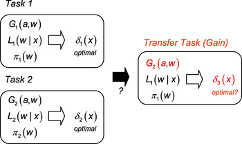
Of course, we need to be able to signal the change in gain function to the observer, or it is unreasonable to expect transfer. In the experiments described in the next section, observers accepted symbolic specifications of altered gain functions and did show transfer. But a lack of transfer may simply indicate a lack of familiarity with the novel gain function. In Fig. 2, we schematize a series of tasks that form a second thought experiment. In Task 1 and Task 2, the observer slowly or quickly learns to select actions that come close to maximizing expected gain. The observer is now familiar with all of the gain, likelihood, and loss functions associated with both tasks but has not experienced them in all possible combinations.
(Color online) Bayesian transfer. An observer practices two BDT tasks, Task 1 and Task 2, to criterion and comes close to maximizing expected gain in both. In the transfer task, we test whether the observer can transfer acquired knowledge about gain functions, likelihood, and priors. In the example shown, the observer is given a new version of Task 1 but with the gain function G 1(a,w) of Task 1 replaced by the gain function G 2(a,w) of Task 2. The observer is familiar with the gain function, likelihood, and prior in the resulting transfer task, but the combination of gain, likelihood, and prior is novel. Is the observer’s performance in the transfer task immediately close to ideal without further practice or learning?

The table-lookup observer in such a thought experiment has learned two tables. We can imagine an alternative observer that has encoded all of the relevant functions. We now present this observer with a novel task that combines the gain function of Task 2, G 2(a,w)with the likelihood  and the prior π 1(w) of Task 1. The table-lookup observer has little choice but to begin to learn a new table. An observer that has access to separate representations of gain, likelihood, and prior and can combine them according to eqn. (1) could, however, work out actions that maximize expected gain in the transfer task. This observer has thereby exhibited an ability to separately encode multiple gains, likelihoods, and priors and “mix and match” them to achieve near-ideal performance without practice or learning. We will demonstrate that human observers do have such transfer capabilities in the next section for one particular class of motor tasks, and these results will help to clarify what is implied in Fig. 2.
There are obviously two other transfer criteria based on substitution of prior and on substitution of likelihood function, respectively. The former criterion, based on prior, is particularly relevant to natural scene statistics applications where the prior is a summary of statistical dependencies in the environment. We illustrate what a prior transfer test might involve.
We cannot hope to test prior transfer if subjects cannot learn new priors as might be the case if priors are either genetically determined or learned very early in development. However, work by Adams et al. (Reference Adams, Graf and Ernst2004) shows that in visual processing of shape, organisms can rapidly learn new priors on illuminant direction. Consequently, it is possible to test prior transfer for two priors on illuminant distribution by embedding subjects in virtual environments with different priors on illumination direction. In the first scene with prior π 1(w), subjects carry out a specific task dictated by gain function G 1(a,w). We could also vary likelihood, but it is not necessary to do so. They learn this combination of task and prior until their performance comes close to maximizing expected gain. They then are placed into second virtual environment with a different prior π 2(w) on illuminant direction and a different task specified by gain function G 2(a,w). They learn this combination of task and prior until their performance comes close to maximizing expected gain. If they succeed in adapting to two different priors with two different tasks, we can then test prior transfer by asking them to carry out a task with gain function G 1(a,w) and the environment corresponding to prior π 2(w) or vice versa. If subjects can immediately maximize expected gain in this third task, they pass the prior transfer test.
The last transfer criterion involves transfer when the likelihood function is changed. The likelihood function is typically interpreted as the operating characteristic of the sensory apparatus, and a test of transfer would in effect test whether the observer could continue to perform optimally when sensory information is degraded or enhanced. Intuitive examples involve losing one’s glasses and attempting to carry out a task for which one has always worn glasses or trying to play soccer at night for the first time. We emphasize that the observer is not expected to carry out tasks as well without glasses or at night but that the transfer criterion contains the prediction that performance without glasses or at night will immediately be close to maximizing expected gain after the transfer.
Cues to context
In the discussion above, we considered how subjects might perform in multiple tasks with objectively different priors, gain functions, and likelihoods. We assume that, with every transition, the subject is able to identify that he is confronted with a previously encountered gain function, prior, or likelihood, and in the experiments discussed next, the subject is simply told about changes in gain functions. The question as to how an organism equipped with representations of multiple gain functions, priors, or likelihoods might decide which choice of gain, prior, or likelihood is appropriate is one we raise but do not further address. Our goal here is to propose tests that could assess whether organism can in fact save, restore, and combine representations of previously encountered gains, priors, and likelihoods at all.
Movement under risk
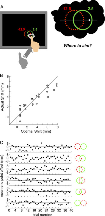
The stimuli represented in Fig. 3A were used in a series of experiments by Trommershäuser and colleagues to test whether human observers can cope with arbitrary gain functions in a simple visuomotor task. When the stimuli appeared on a computer touch screen, the observer had 700 ms to reach out and touch the screen. If the observer was late, he incurred a large monetary penalty (Trommershäuser et al., Reference Trommershäuser, Maloney and Landy2003a,Reference Trommershäuser, Maloney and Landyb, Reference Trommershäuser, Maloney and Landy2008). Otherwise, the location of the touch on the screen determined the observer’s reward or penalty. These rewards and penalties were signaled by colored circles on the screen. In Fig. 3, we draw red circles as dashed and green as solid, so that they be readily differentiated in black and white versions of the article. The stimuli are in color in the online version of the article. Hitting within a red circle resulted in a penalty that varied from condition to condition, and hitting within a green circle resulted in a small reward. Touching outside both circles but within the time limit resulted in neither reward nor penalty.
(Color online) Six tests of transfer with a spatial gain function. (A) A stimulus configuration such as the one shown appears on a computer screen in front of the observer who was instructed to reach out and touch the screen within 700 ms. The gain function is coded by colored circles whose position and relative orientation change from trial to trial. A hit within the solid green circle results in a gain of 2.5 cents, within the dashed red circle, and a loss of 12.5 cents. The observer moves rapidly and cannot completely control his movement. Even if he aims at a particular point on the screen, the result is a probability distribution of actual end points that induce probabilities of hitting within each region. A possible aim point in marked by a white dot. How much should the observer aim away from the dashed red circle to maximize expected gain? (B) Actual choice of aim point (horizontal deviation along the white line) plotted versus optimal choice of end point computed via BDT. (C) Trial-by-trial deviation of movement end point (in the horizontal direction), a function of trial number after introduction of rewards and penalties for six different gain functions. The online version of this figure is in color. Figure reproduced with permission from Trommershäuser et al. (Reference Trommershäuser, Maloney and Landy2008).

The observer could not completely control his speeded movement, and a movement aimed at the center of the green circle had a substantial probability of missing the green circle altogether. This probability varied from observer to observer depending on each observer’s intrinsic motor accuracy. The location of the red circle with respect to the green varied from trial to trial as did the degree of overlap of the circles. There were a total of six experimental conditions each with a distinct gain function but, in terms of BDT, with the same prior and the same likelihood functions. There are two sources of prior uncertainty, motor error and visual error in locating the target. Trommershäuser et al. (Reference Trommershäuser, Maloney and Landy2008) derive a modified form of eqn. (1) that serves as a BDT model for this task. In terms of BDT, the observer carries out interleaved tasks with six different loss functions but the same likelihood and prior.
Prior to the experimental session, however, the observer practiced the movement by hitting identical stimuli where there was a small reward associated with hitting within the green circle (within the time limit) but no reward or penalty associated with the red circle which was nevertheless always present. After several hundred trials, observers learned to respond within the time window of 700 ms, and their motor uncertainty had improved and stabilized.
In the main part of the experiment, the observer was effectively asked to transfer from the gain function in training to each of the six interleaved penalty conditions. The observer’s strategy may be represented by choice of where to aim, and for any value of penalty and relative position of red and green circles, the aim point that maximized gain fell on the white line bisecting the two circles in Fig. 3A. We can therefore compare observers’ performance by plotting the mean end point of reaches in each condition to the aim point that maximizes expected gain, and this is shown for all observers in Fig. 3B. The observers’ performance shows no obvious deviations or trends from that which would maximize expected gain as predicted by BDT.
The purpose of the experiment of Trommershäuser et al. (Reference Trommershäuser, Maloney and Landy2003a) was not to test a transfer property, but if we take into account the gain function imposed in the training session, we find that the design of the experiment was appropriate to test transfer to novel gain functions. The observer had the opportunity to maximize expected gain during training and did so. We would expect the same good performance from a table-lookup observer who simply learned to maximize gain by aiming at the center of the green circle (all observers exhibited isotropic Gaussian motor error, and aiming at the center of the green circle did maximize expected gain).
We can then examine observers’ performance on the first few trials when exposed to the six interleaved experimental conditions in the main part of the experiment and look for any evidence that observers are adjusting aim point. The evidence for such adjustment would be trends in aim point, especially along the white line. In Fig. 3C, we plot horizontal displacement of end points versus trials where displacement is coded with respect to the mean horizontal end point for each condition. The prediction of transfer is then that these displacements will show no trends but will be instead symmetrically distributed around zero (the asymptotic aim point), as appears to be the case. We found no evidence of patterned trends across the first few trials across subjects, and the correlation between successive trials was not significantly different from zero.
The implication is that observers who have learned to aim the center of targets in training are able to transfer their experience of their own visuomotor error to novel conditions with gain functions involving penalties. It is difficult to explain this performance unless observers have spontaneously encoded information about their own visuomotor performance during training and combined this information with novel gain functions. In terms of Fig. 2, we did not even need to employ a second task. Observers made use of the symbolic encoding in terms of colored circles, again with no prior experience of regions that incurred penalty.
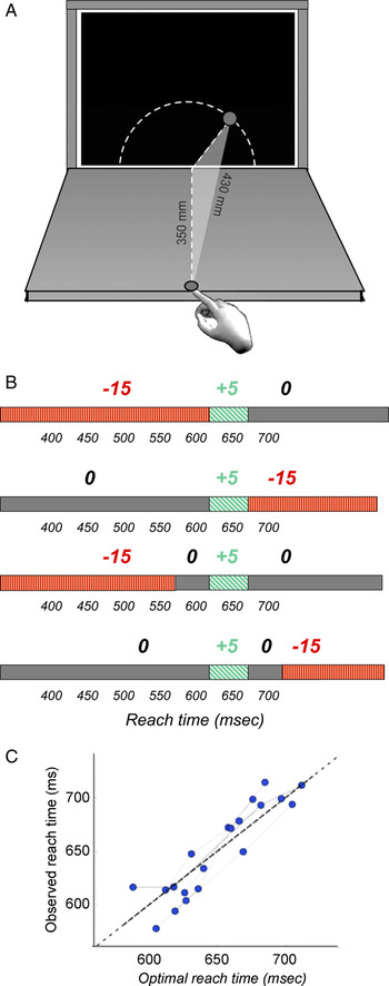
More recent work has extended these basic results to analogous experiments where the gain function is specified in the temporal domain (Hudson et al., Reference Hudson, Maloney and Landy2008). Observers attempted to hit small targets on a computer screen (Fig. 4A), but no time limit was imposed. In the experimental task, the observer saw a time line specifying the reward or penalty associated with movements to touch the target differing in duration (Fig. 4B). The rewards associated with green temporal windows and the penalties associated with red temporal windows were coded in terms of points, and the observers knew that they would receive a monetary reward at the end of the experiment proportional to total points earned. In the print version of this article, we represent penalty windows by red vertical hatching and reward windows by green slanted hatching (Fig. 4B). The stimuli are in color in the online version of the article.
(Color online) Four tests of transfer with a temporal gain function. (A) Observers had to reach out and touch small targets presented at random on a computer screen along the arc of a circle equidistant from the start point. Rewards and penalties were determined by the time of arrival at the target. (B) Four temporal gain functions were used in four different experimental conditions. The horizontal axis is movement time, and the rewards or penalties associated with each possible movement time were displayed as a time line similar to those shown here. If the observer touched the target in the time window marked in green (slanted hatching), he received a reward of 5 points. If instead he arrived in the time window marked in red (vertical hatching), he lost 15 points. (C) A plot of actual movement durations versus the mean movement time that maximized expected gain for each condition and each observer. The online version of this figure is in color. Figure reproduced with permission from Hudson et al. (Reference Hudson, Maloney and Landy2008).

As in Trommershäuser et al. (Reference Trommershäuser, Maloney and Landy2003a), observers first completed an extensive training session where they were challenged to complete movements of specified durations to the target and given extensive feedback specifying their actual movement times.
We can therefore examine how well observers transferred their experience in training to the four experimental conditions each with a different temporal penalty function. The summary of actual versus optimal movement times across the four conditions and all observers is shown in Fig. 4C. There were no obvious trends consistent with learning in the transfer (Hudson et al., Reference Hudson, Maloney and Landy2008). Hudson et al. (Reference Hudson, Maloney and Landy2008, pp. 4–5) compared observed performance across time to reinforcement learning models and found that such models did not predict observed performance: “To investigate the possibility that subjects used a hill-climbing strategy during the main experiment, instead of maximizing expected gain by taking account of their own temporal uncertainty function and experimentally imposed gain function, we performed a hill-climbing simulation using each subject's temporal uncertainty function. In the simulation, intended duration was moved away from the penalty region by 3 Δt ms after each penalty and towards the center of the target region by Δt ms for each miss of the target that occurred on the opposite side from the penalty (corresponding to the 3:1 ratio of penalty to reward). The value of Δt was initially set to be relatively large. With each change of direction of step, Δt was reduced by 25% to a minimum step size of 1.5 ms. While this simulation approximately reproduced the final average reach times observed experimentally, it does not provide a good model of subject performance. First, there were significant autocorrelations of reach durations beyond lag zero in the simulation data but not in the experimental data. Second, a learning algorithm would be expected to produce substantially higher σ values during test than those observed during training. This is what we found with our hill-climbing simulation. Using subjects’ training σ values to produce the simulated data, the simulation produced 17 out of 20 main-experiment σ values that were above the training values, whereas our subjects’ main-experiment σ values … were entirely consistent with temporal uncertainty functions measured during training.”
Riesz representation theorem
The transfer criteria that we propose embody experimental tests that allow us to determine whether observers can separately encode and manipulate gain functions, likelihoods, and priors according to eqn. (1). We have in effect proposed three additional criteria (beyond near-ideal performance) for what it might mean to separately represent and manipulate these functions in accordance with BDT.
We do not assume that an observer who has passed one of the transfer tests will pass the other two. If, for example, human observers can transfer gain and prior functions but not likelihood functions, then we will have learned something important about the limitations of the human visuomotor system.
We can also characterize how much information each kind of transfer task can give us about the observer’s representation of the elements of BDT. Consider, for example, the transfer task where we substitute a novel gain function for one learned. We can combine the unchanging likelihood function and prior into a posterior distribution  by Bayes’ theorem. Then, eqn. (1) can be written as:
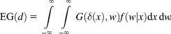
and changing the order of integration,
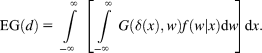
To maximize eqn. (5), we need to only maximize
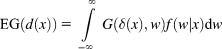
for each specific choice of x (Maloney, Reference Maloney, Heyer and Mausfeld2002). Intuitively, on each trial, we have only one specific choice of x and if we choose an action that maximizes expected gain on that trial, then we maximize overall expected gain across all trials. If the observer can compute eqn. (6) for any choice of action, then he or she can compute
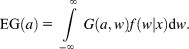
Eqn. (6) is an inner product of functions (Apostol, Reference Apostol1969, Chapters 1–2) analogous to an inner product of finite-dimensional vectors  . Suppose that we freely vary G(a,w), the gain function as a function of w while holding a and
 constant. What can we learn about
 by observing EG(a)? The reader familiar with the finite-dimensional case likely recognizes that, after a finite number of choice of G, w is determined by the values
 . This result is the basis for the method of classification images (Ahumada & Lovell, Reference Ahumada and Lovell1971; Ahumada, Reference Ahumada2002). In the infinite-dimensional case as well, observing the output of free variation of G(a,w) for fixed a also determines the posterior
 , a result known as the Riesz representation theorem (Riesz, Reference Riesz1907, Reference Riesz1909; Rudin, Reference Rudin1966, pp. 129–131). If the observer has the ability to combine arbitrary gain functions with a fixed posterior following eqn. (7), then the values of EG(a) that result determine the posterior distribution.
We propose the derivation above in order to characterize how changes in gain function constrain the performance of the BDT observer. Another way to summarize the result just derived is to imagine an observer who has an incorrect estimate of the posterior distribution but selects actions according to eqn. (1). We have shown that for some choices of gain function, his performance will fail to maximize expected gain.
We do not propose the thought experiment above as an experiment that can be carried out practically. As stated, the resulting experiment would involve testing performance with infinitely many gain functions, an impossibility. However, it would be of interest to examine human performance with multiple gain functions as a means of gaining partial information about the observer's estimate of posterior distribution (e.g., its low-pass components). Variations in prior could serve a similar role in probing how observers decide how to act.
Conclusions
BDT is a mathematical framework used to model ideal performance in a wide range of visuomotor tasks. Its elements (gain function, likelihood, and prior) are readily interpretable in terms of information available to the observer, and BDT allows the experimenter to compute ideal performance in specific tasks and compare human performance to ideal.
Recently, several researchers have proposed BDT as a process model of perception as Bayesian inference (Knill & Richards, Reference Knill and Richards1996), while others have questioned whether it is relevant as a process model (Shimojo & Nakayama, Reference Shimojo and Nakayama1992). We described how reinforcement learning could be used to explain near-ideal performance in a table-lookup observer that combined cues and argued that good performance alone is not strong evidence that “perception is Bayesian inference.”
We proposed additional experimental “transfer criteria” intended as experimental tests of the claim that perception is Bayesian inference. These tests go beyond a simple benchmark comparison of the observer’s performance to ideal and employ a novel comparison of performance in a series of experimental tasks. Across the series of tasks, the observer is exposed to several gain functions, priors, and likelihood functions, and we examined whether observers can transfer knowledge about gain functions, priors, and likelihood functions from one task to another without additional learning.
We can distinguish the transfer tests we propose here from measures of generalization across tasks. It is plausible that the nervous system, having learned a task with gain function G 1(a,w), likelihood function  , and prior π 1(x), can more rapidly learn an immediately following task with a novel gain function G 2(a,w) but with the same likelihood and prior. We could refer to this acceleration in learning as generalization, but it is not an example of transfer.
In the gain transfer task, we ask for evidence that the nervous system, having first learned to carry out an initial task with G 1(a,w), likelihood function  , and prior π 1(x), and then, having learned a second task with distinct choices of gain function G 2(a,w), likelihood function
 , and prior π 2(x), can immediately carry out tasks corresponding to novel combinations of the two gains, two likelihoods, and two priors. The transfer task effectively tests whether the nervous system can save and restore representations of multiple gain functions independent of the specific likelihoods and priors present in the tasks where the gain functions were first encountered. The conclusion we draw is stronger than the conclusion we would draw given only evidence of generalization.
We described experiments where human observers are asked to switch from one gain function to another (Trommershäuser et al., Reference Trommershäuser, Maloney and Landy2003a; Hudson et al., Reference Hudson, Maloney and Landy2008). They are able to do so without evident trends in performance that would suggest learning. An intuitive summary of what we have learned is that human observers can separately represent stochastic information corresponding to likelihood and prior and combine this information with novel, arbitrary gain functions according to BDT. The series of experiments involved in testing transfer allows us to draw this conclusion, while a benchmark comparison of performance in any single experiment would not. It is of interest to determine whether human observers can also transfer knowledge of likelihoods and of priors as they do knowledge of gains.
Operationalization and representation
Suppose that the organism fails one or more of our transfer tests. Can we conclude that the organism has no “separate” representation of gain functions or cannot save multiple representations of gain functions across tasks? We would argue no. What we have established is that whatever the structure and content of the organism’s representation of BDT tasks, we see no evidence in behavior that the organism can save and restore representations of gain functions independent of the prior and likelihood functions present when each gain function was first learned. An analogy may be found in long-term memory where a memory trace may be present but not accessible because of interference.
We can imagine an artificial learning system whose programmer is certain that gain, likelihood, and prior are learned in separate data structures and where the combined gain, likelihood, and prior for any previous task are stored indefinitely and can be recalled when needed again to carry out the identical task. Because of a programming oversight, however, there is no way to extract gain from the representation of one task and likelihood and prior from the representation of a second and combine them to create the representation of a new task which the organism can immediately use to solve the task corresponding to the novel combination of gain, likelihood, and prior. The information is there, but the architecture of the system cannot make use of it, and this artificial learning system will fail the gain transfer task.
The necessity of transfer?
The evident advantage of transfer is that it allows organisms to achieve near-optimal performance rapidly in novel tasks. It is possible that transfer plays a second critical role in allowing organisms to learn complex tasks as a series of tasks increasing in complexity. In Trommershäuser et al., for example, observers first were given the opportunity to learn their own visual and motor uncertainties in a training task involving gain functions specifying only reward regions. Only then were they asked to address tasks involving gain functions with both penalty and reward regions. How would these observers have fared if asked to start with the experimental task directly without any previous training?
Mamassian (Reference Mamassian2008) reported a visuomotor synchrony task where participants had to press a key in anticipation of a visual target. In that experiment, participants were not offered the possibility to practice on a simpler version of the task prior to the main experimental task. Even though motor learning was observed over the course of the experiment, there was no evidence of optimal use of the gain function. These observers failed the benchmark criterion. Could they have done better if the experiment had first allowed observers to train with simpler gain functions? We advance the conjecture that prior experience with a simpler version of the experimental task may lead to performance that more rapidly converges to ideal. Results in the animal learning literature concerning learning by chaining simple tasks together are analogous to this claim (Mackintosh, Reference Mackintosh1974).
Mixture models
Several groups of researchers are currently investigating whether selection of actions can be modeled as a mixture of experts (Jordan & Jacobs, Reference Jordan and Jacobs1994; Meila & Jordan, Reference Meila, Jordan, Murray-Smith and Johanssen1996; Yuille & Rangarajan, Reference Yuille and Rangarajan2003), and we can consider whether such a model could exhibit transfer. If, for example, the organism has learned appropriate table-lookup strategies for a task with gain function G 1(a,w), likelihood function  , and prior π 1(x) and a second task with distinct choices of gain function G 2(a,w), likelihood function
 , and prior π 2(x), could it exhibit transfer by mixing actions in action space? Evidently, there are two conditions that must be satisfied for transfer to be possible. The first is that the choice of actions in the transfer task that maximizes expected gain must be expressible as a weighted mixture of the actions in the two previously learned tasks, and the second is that the organism can somehow arrive at the correct choice of weights used in mixing actions. We emphasize, though, that such “mixture of actions” models are not in conflict with BDT. Indeed, if the resulting actions are those dictated by eqn. (1), the “mixture of actions” model would simply be an implementation of BDT.
We end by emphasizing the importance of operationalization of models of BDT. We sought to define concepts such as gain functions, prior, and likelihood functions in terms of performance in experimental tasks. The question of whether the observer represents the elements of BDT and combines them by means of some analogue of eqn. (1) is then addressable experimentally. “If a specific question has meaning, it must be possible to find operations by which an answer may be given to it. It will be found in many cases that the operations cannot exist, and the question therefore has no meaning.” (Bridgman, Reference Bridgman1927).
Acknowledgments
Supported in part by NIH EY02866 (L.T.M.) and a chair of excellence from the French Ministry of Research (P.M.).