1. Introduction
Magnetic reconnection is a plasma process in which topological changes of magnetic field lines release the energy stored in the magnetic field in the form of kinetic energy and heat. It is considered to be the cause of the release of magnetic energy in solar flares, sub-storms in the Earth’s magnetosphere, sawtooth crashes in tokamaks and many astrophysical systems, e.g. accretion disks. The topological changes of magnetic field lines take place in a current sheet and require dissipation in the current sheet. In the absence of collisions, lack of dissipation allows the current sheet to thin down to microscopic scales, such as the electron and ion inertial lengths, and an effective dissipation is provided by micro-physical plasma processes. As a result, the reconnecting current sheet develops a two scale structure (along its thickness), viz., an electron current sheet with thickness of the order of an electron inertial length,
 $d_{e}=c/{\it\omega}_{pe}$
embedded inside an ion current sheet with thickness of the order of an ion inertial length,
 $d_{i}=c/{\it\omega}_{pi}$
. Reconnection of field lines takes place in electron current sheets and couples to ions, and then further, to very large MHD scales.
The electron and ion current sheets are susceptible to a variety of instabilities. These instabilities have potential to affect the rate and structure of reconnection. The role of ion scale instabilities in reconnection has been discussed in a review by Büchner & Daughton (Reference Büchner, Daughton, Birn and Priest2006). On electron scales, the electron current sheet (ECS) can be unstable to electromagnetic instabilities driven by the gradients in the ECS or to an electrostatic Buneman instability (Buneman Reference Buneman1958) driven by the relative drift of electrons and ions. The electrostatic Buneman instability grows (typical growth rates
 ${\sim}$
fraction of
 ${\it\omega}_{pe}$
) much faster than the electromagnetic instabilities without affecting the magnetic fields. Growth of the electromagnetic tearing and non-tearing instabilities leads to the generation of flux ropes/plasmoids (Daughton et al.
Reference Daughton, Roytershteyn, Karimabadi, Yin, Albright, Bergen and Bowers2011; Markidis et al.
Reference Markidis, Henri, Lapenta, Divin, Goldman, Newman and Laure2013) and filamentation of the ECS (Che, Drake & Swisdak Reference Che, Drake and Swisdak2011), respectively. The conditions under which an ECS filaments or generates flux ropes/plasmoids depend on the presence of an external guide field and the thickness of the current sheet. Recently, it was shown that, depending on the thickness of the ECS, electron shear flow instabilities (ESFI) can grow both as 3-D oblique tearing modes which generate flux ropes/plasmoids and/or as non-tearing modes which filament the ECS (Jain & Büchner Reference Jain and Büchner2014a
,Reference Jain and Büchner
b
). Without an external guide field, the tearing mode instability dominates the non-tearing modes only if the sheet is thin, with a half-thickness close to an electron inertial length (Jain & Büchner Reference Jain and Büchner2014a
,Reference Jain and Büchner
b
). Otherwise non-tearing mode instabilities dominate.
In this paper, we numerically perform linear stability analysis for ESFI of an ECS in the presence of an external guide field in the limit of
 ${\it\beta}_{e}\ll 1$
, where
 ${\it\beta}_{e}$
is the ratio of the electron and magnetic pressures. We employ an electron-magnetohydrodynamic (EMHD) (Kingsep, Chukbar & Yan’kov Reference Kingsep, Chukbar and Yan’kov1990) model. Studies of electron shear flow instabilities in EMHD approximation have earlier been reported but without a guide field (Basova et al.
Reference Basova, Varentsova, Gordeev, Gulin and Shuvaev1991; Drake, Kleva & Mandt Reference Drake, Kleva and Mandt1994; Das & Kaw Reference Das and Kaw2001; Jain et al.
Reference Jain, Das, Kaw and Sengupta2003, Reference Jain, Das, Sengupta and Kaw2012; Jain, Das & Kaw Reference Jain, Das and Kaw2004; Gaur & Das Reference Gaur and Das2012). These instabilities have also been referred to as current driven sausage and kink instabilities, because in EMHD, electron flow is equivalent to current (Das & Kaw Reference Das and Kaw2001; Jain et al.
Reference Jain, Das, Kaw and Sengupta2003, Reference Jain, Das and Kaw2004).
In the next section we briefly describe the EMHD model and obtain the linearized EMHD equations for ESFI. Section 3 discuss effects of the guide field on ESFI. We conclude this paper in § 4.
2. EMHD model
The EMHD model is a fluid model for electron dynamics in a stationary background of ions. It is valid for spatial scales smaller than
 $d_{i}$
and time scales smaller than
 ${\it\omega}_{ci}^{-1}$
. In EMHD, electron dynamics is described by the electron momentum equation coupled with Maxwell’s equations. An evolution equation for the magnetic field
 $\boldsymbol{B}$
can be obtained by eliminating the electric field from the electron momentum equation using Faraday’s law (Kingsep et al.
Reference Kingsep, Chukbar and Yan’kov1990).
 $$\begin{eqnarray}\displaystyle \frac{\partial }{\partial t}(\boldsymbol{B}-d_{e}^{2}{\rm\nabla}^{2}\boldsymbol{B})=\boldsymbol{{\rm\nabla}}\times [\boldsymbol{v}_{e}\times (\boldsymbol{B}-d_{e}^{2}{\rm\nabla}^{2}\boldsymbol{B})], & & \displaystyle\end{eqnarray}$$
where,
 $\boldsymbol{v}_{e}=-(\boldsymbol{{\rm\nabla}}\times \boldsymbol{B})/{\it\mu}_{0}n_{0}e$
is the electron fluid velocity. In addition to ignoring the ion dynamics, (2.1) assumes uniform electron number density
 $n_{0}$
and incompressibility of the electron fluid. The displacement current is ignored under the assumption
 ${\it\omega}\ll {\it\omega}_{pe}^{2}/{\it\omega}_{ce}$
. In EMHD, the frozen-in condition of magnetic field breaks down due to electron inertia (which is contained in the definition of
 $d_{e}\propto \sqrt{m_{e}}$
). Inclusion of electron inertia extends the validity of the EMHD model to spatial scales smaller than
 $d_{e}$
. In the absence of electron inertia (
 $d_{e}\rightarrow 0$
), (2.1) represents the condition that magnetic field is frozen in the electron fluid.
The equilibrium magnetic field is taken to be
 $\boldsymbol{B}_{0}=B_{y0}\tanh (x/L){\hat{y}}+B_{z0}\hat{z}$
corresponding to a current density
 $\boldsymbol{J}_{0}=(B_{y0}/{\it\mu}_{0}L)\text{sech}^{2}(x/L)\hat{z}$
, where
 $L$
is the half-thickness of the electron current sheet. For stationary ions, electron fluid velocity is related to current density by the relation
 $\boldsymbol{J}=-n_{0}e\boldsymbol{v}_{e}$
. In the limit of cold electrons, a bipolar electrostatic electric field collocated with the electron current sheet balances the Lorentz force in the current sheet. Small deviations from charge neutrality in the electron current sheet can support the bipolar electric field (Li & Horiuchi Reference Li and Horiuchi2008). This force balance is different from the force balance between the pressure gradient and Lorentz force as in the case of a Harris current sheet. The bipolar electrostatic electric field and the new force balance in the electron current sheet have been observed in particle-in-cell (PIC) simulations (Li & Horiuchi Reference Li and Horiuchi2008; Chen et al.
Reference Chen, Daughton, Lefebvre and Torbert2011), laboratory experiments (Yoo et al.
Reference Yoo, Yamada, Ji and Myres2013) and space observations (Chen et al.
Reference Chen, Bessho, Lefebvre, Vaith, Asnes, Santolik, Fazakerley, Puhl-Quinn, Bhattacharjee, Khotyaintsev, Daly and Torbert2009).
Note that the EMHD model cannot describe finite-Larmor-radius (FLR) effects which may be important in electron current sheets with thickness
 $L\sim {\it\rho}_{e}$
, where
 ${\it\rho}_{e}=m_{e}v_{the}/eB_{z0}$
is the electron Larmor radius in the guide field
 $B_{z0}$
and
 $v_{the}$
is electron thermal velocity. We consider electron current sheets with thicknesses
 $L\sim d_{e}$
, and thus our results are valid for electron plasma with
 ${\it\beta}_{e}=\sqrt{{\it\rho}_{e}/d_{e}}\ll 1$
.
For the linear stability analysis of ESFI in ECS, we linearize the EMHD equation (2.1) about the current sheet equilibrium and then Fourier transform them in
 $y$
,
 $z$
and
 $t$
. This yields two coupled equations in velocity and magnetic field perturbations,
 $v_{x}(x,k_{y},k_{z},{\it\omega})$
and
 $b_{x}(x,k_{y},k_{z},{\it\omega})$
, where
 $k_{y}$
and
 $k_{z}$
are the respective wavenumbers along
 $y$
and
 $z$
directions and
 ${\it\omega}={\it\omega}_{r}+\text{i}{\it\gamma}$
is the complex frequency.
 $$\begin{eqnarray}\displaystyle d_{e}^{2}\frac{\text{d}^{2}v_{x}}{\text{d}x^{2}}-(1+k^{2}d_{e}^{2})v_{x} & = & \displaystyle -\frac{d_{e}^{2}{\it\omega}_{ce}^{2}}{B_{y0}^{2}}\frac{F-d_{e}^{2}F^{\prime \prime }}{\bar{{\it\omega}}}b_{x}-\frac{d_{e}^{2}{\it\omega}_{ce}^{2}}{B_{y0}^{2}}\frac{F(F-d_{e}^{2}F^{\prime \prime })}{\bar{{\it\omega}}^{2}}v_{x}\nonumber\\ \displaystyle & & \displaystyle +\,\frac{k_{z}(v_{0}-d_{e}^{2}v_{0}^{\prime \prime })}{\bar{{\it\omega}}}v_{x}\end{eqnarray}$$
 $$\begin{eqnarray}\displaystyle & \displaystyle d_{e}^{2}\frac{\text{d}^{2}b_{x}}{\text{d}x^{2}}-(1+k^{2}d_{e}^{2})b_{x}=\frac{F-d_{e}^{2}F^{\prime \prime }}{\bar{{\it\omega}}}v_{x}. & \displaystyle\end{eqnarray}$$
Here
 $\bar{{\it\omega}}={\it\omega}-k_{z}v_{0}$
,
 $k^{2}=k_{y}^{2}+k_{z}^{2}$
,
 ${\it\omega}_{ce}=eB_{y0}/m_{e}$
and
 $F=\boldsymbol{k}\boldsymbol{\cdot }\boldsymbol{B}_{0}$
. The sub-script ‘
 $e$
’ is dropped from the electron flow velocity and a prime (
 $\prime$
) over an equilibrium variable denotes a derivative with respect to
 $x$
.
Equations (2.2) and (2.3) are discretized in
 $x$
, reducing them to algebraic equations which can be cast in a form of matrix eigenvalue problem with
 ${\it\omega}$
as the eigenvalue. The resulting matrix eigenvalue problem is solved numerically using a MATLAB code to obtain eigenvalues
 ${\it\omega}$
corresponding to the confined eigenfunctions
 $v_{x}$
and
 $b_{x}$
.
The current sheet equilibrium has two parameters, viz., half-thickness
 $L$
of the electron current sheet and the guide field
 $B_{z0}$
. The values of
 $L/d_{e}=0.5{-}6$
and
 $B_{z0}/B_{y0}=0{-}10$
relevant for the electron current sheets formed in collisionless magnetic reconnection are chosen. The spectrum of the unstable modes over a wide range of values of
 $k_{y}$
and
 $k_{z}$
is obtained for each set of the values of
 $L/d_{e}=0.5{-}6$
and
 $B_{z0}/B_{y0}=0{-}10$
.
Results are presented in normalized variables. The magnetic field is normalized by
 $B_{y0}$
, length by the electron inertial length
 $d_{e}$
, time by the inverse electron cyclotron frequency
 ${\it\omega}_{ce}^{-1}=(eB_{y0}/m_{e})^{-1}$
and velocity by the electron Alfven velocity
 $v_{Ae}=d_{e}{\it\omega}_{ce}$
. Under this normalization,
 $\boldsymbol{J}=-\boldsymbol{v}_{e}$
holds.
3. Electron shear flow instabilities
Electron shear flow instabilities can grow both as tearing or non-tearing modes, depending upon the wavenumbers (
 $k_{y},k_{z}$
), current sheet half-thickness (
 $L$
) and the guide field (
 $B_{z0}$
). In this paper, our objective is to identify regions in
 $L$
–
 $B_{z0}$
parameter space where tearing or non-tearing modes dominate. We first define the characteristic features of the tearing mode in order to distinguish it from other non-tearing modes. Then we study how the nature (tearing or non-tearing) of the fastest growing mode changes as we change
 $L$
and/or
 $B_{z0}$
.
3.1. Tearing versus non-tearing modes
The growth of the tearing mode leads to the development of magnetic islands. For this to happen, the normal magnetic field
 $B_{x}$
must not be zero at the mode resonance surface at
 $x=x_{0}$
. At the same time, inflow must change the sign at
 $x=x_{0}$
and thus
 $v_{x}(x_{0})=0$
. Otherwise a magnetic island will not develop.
We define an unstable mode to be a tearing mode if (1)
 $v_{x}$
is an odd function of
 $x$
about the mode resonance surface
 $x=x_{0}\leqslant L$
(inside the ECS) so that
 $v_{x}(x_{0})=0$
and (2)
 $b_{x}(x_{0})\neq 0$
. All other modes are considered to be of the non-tearing type. Note that the free energy source for all the unstable modes (both tearing and non-tearing) is the electron shear flow, which is equivalent to electric current for stationary ions.
Applying the tearing mode conditions, viz.,
 $v_{x}(x_{0})=0$
and
 $b_{x}(x_{0})\neq 0$
, in (2.2) and (2.3), we obtain the necessary conditions for the existence of tearing eigenfunctions.
 $$\begin{eqnarray}\displaystyle & \displaystyle [F-d_{e}^{2}F^{\prime \prime }]_{x=x_{0}}=0, & \displaystyle\end{eqnarray}$$
 $$\begin{eqnarray}\displaystyle & \displaystyle \left[\frac{1}{b_{x}}\frac{\text{d}^{2}b_{x}}{\text{d}x^{2}}\right]_{x=x_{0}}=1+k^{2}d_{e}^{2}, & \displaystyle\end{eqnarray}$$
where we have used
 $[\text{d}^{2}v_{x}/\text{d}x^{2}]_{x=x_{0}}=0$
as
 $v_{x}$
is an odd function about
 $x=x_{0}$
. Equations (3.1) and (3.2) are only necessary conditions for the existence of tearing type eigenfunctions which could either be stable or unstable. Since the right-hand side of (3.2) is always finite,
 $b_{x}(x_{0})$
and
 $[\text{d}^{2}b_{x}/\text{d}x^{2}]_{x_{0}}$
cannot be zero, except when both
 $b_{x}(x_{0})$
and
 $[\text{d}^{2}b_{x}/\text{d}x^{2}]_{x_{0}}$
approach zero simultaneously.
Equation (3.1) is the mode resonance condition and its solution provides the mode resonance surfaces
 $x=x_{0}$
. Note that (3.1) is different from the usual resonance condition (
 $F=\boldsymbol{k}\boldsymbol{\cdot }\boldsymbol{B}_{0}=0$
) for the tearing mode. Equation (3.1) has a term due to the electron inertia (
 $d_{e}^{2}F^{\prime \prime }$
) which in EMHD provides an effective dissipation for the growth of tearing instability. It reduces to
 $\boldsymbol{k}\boldsymbol{\cdot }\boldsymbol{B}_{0}=0$
only for equilibrium scale lengths much larger than the electron inertial length (scale length of the effective dissipation). In fact, the mode resonance condition for the MHD tearing mode should also be different from
 $\boldsymbol{k}\boldsymbol{\cdot }\boldsymbol{B}_{0}=0$
and have terms due to the plasma resistivity which provides dissipation for the growth of the MHD tearing instability. This can be seen by applying conditions for the tearing mode eigenfunctions in equation (14) of Furth, Killeen & Rosenbluth (Reference Furth, Killeen and Rosenbluth1963). Assuming uniform density, we obtain for MHD
 $$\begin{eqnarray}\displaystyle \boldsymbol{k}\boldsymbol{\cdot }(\boldsymbol{B}_{0}-L_{{\it\eta}}^{2}\boldsymbol{B}_{0}^{\prime \prime })=0, & & \displaystyle\end{eqnarray}$$
where
 $L_{{\it\eta}}={\it\eta}/4{\rm\pi}{\it\omega}$
is the resistive scale length and
 ${\it\eta}$
is the resistivity. Equation (3.3) reduces to
 $\boldsymbol{k}\boldsymbol{\cdot }\boldsymbol{B}_{0}=0$
only when the equilibrium scale length is much larger than the resistive scale length.
Substituting for the equilibrium magnetic field
 $\boldsymbol{B}_{0}$
in (3.1), the values of
 $x_{0}$
can be obtained from following equation
 $$\begin{eqnarray}\displaystyle \tanh ^{3}\left(\frac{x_{0}}{L}\right)-\left(1+\frac{L^{2}}{2d_{e}^{2}}\right)\tanh \left(\frac{x_{0}}{L}\right)-\frac{k_{z}B_{z0}L^{2}}{2k_{y}B_{y0}d_{e}^{2}}=0. & & \displaystyle\end{eqnarray}$$
For zero guide field,
 $B_{z0}=0$
, the only real solution of (3.4) is
 $x_{0}=0$
, as expected. For finite guide field,
 $x_{0}\leqslant 0$
, as
 $x_{0}>0$
is not allowed by (3.4) for
 $B_{z0}>0$
. The real root of (3.4),
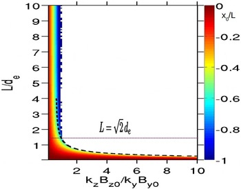
 $x_{0}/L\leqslant 1$
, is plotted in
 $L/d_{e}$
–
 $k_{z}B_{z0}/k_{y}B_{y0}$
parameter space in figure 1. The white space in this plot identifies the regions of
 $L/d_{e}$
–
 $k_{z}B_{z0}/k_{y}B_{y0}$
space where no real solution of (3.4) exist. In the limit
 $L\gg \sqrt{2}d_{e}$
and
 $k_{z}B_{z0}/k_{y}B_{y0}\gg 1$
, (3.4) reduces to
 $\tanh ^{3}(x_{0}/L)=k_{z}B_{z0}L^{2}/2k_{y}B_{y0}d_{e}^{2}$
which has no real solution because
 $\tanh (x_{0}/L)\leqslant 1$
. When
 $k_{z}B_{z0}/k_{y}B_{y0}<1$
, real solutions of
 $x_{0}$
exist for any value of
 $L$
. In this limit, the value of
 $x_{0}/L$
does not depend on
 $L$
for
 $L\gg \sqrt{2}d_{e}$
but does depend on
 $k_{z}B_{z0}/k_{y}B_{y0}$
. For
 $L\gg \sqrt{2}d_{e}$
and
 $k_{z}B_{z0}/k_{y}B_{y0}<1$
, (3.4) can be simplified by neglecting the cubic term to give
 $x_{0}/L=-\tanh ^{-1}(k_{z}B_{z0}/k_{y}B_{y0})$
, which is independent of
 $L$
. This result can be derived from the condition
 $\boldsymbol{k}\boldsymbol{\cdot }\boldsymbol{B}_{0}=0$
which can be obtained from the resonance condition, (3.1), in the limit
 $L\gg d_{e}$
. We find that the relation,
 $k_{z}B_{z0}/k_{y}B_{y0}=(1/\sqrt{3})(1+4d_{e}^{2}/3L^{2})$
, approximates very well the boundary (black dashed line in figure 1) between the regions of the existence and non-existence of the mode rational surface for
 $L<\sqrt{2}d_{e}$
.
Real root
 $|x_{0}/L|\leqslant 1$
of (3.4). Colour scales are saturated at
 $x_{0}/L=-1$
. The black dashed line is the plot of
 $k_{z}B_{z0}/k_{y}=(1/\sqrt{3})(1+4/3L^{2})$
. No real root exists in the white regions in
 $L$
–
 $k_{z}B_{z0}/k_{y}$
space.

The resonance condition, (3.1), is only a necessary condition for the existence of tearing eigenfunctions. Therefore it cannot be used with certainty to predict the existence of tearing instability. However, its violation guarantees that a tearing mode cannot exist. The conditions for the non-existence of the tearing mode, obtained from the non-existence of the resonance surface, can be stated as follows.
 $$\begin{eqnarray}\displaystyle \frac{k_{z}B_{z0}}{k_{y}B_{y0}} & {>} & \displaystyle 1,\quad \text{if }L>\sqrt{2}d_{e}\end{eqnarray}$$
 $$\begin{eqnarray}\displaystyle & {>} & \displaystyle \frac{1}{\sqrt{3}}\left(1+\frac{4d_{e}^{2}}{3L^{2}}\right),\quad \text{if }L<\sqrt{2}d_{e}.\end{eqnarray}$$
3.2. Growth rates
In general, the 3-D unstable modes driven by electron shear flow in EMHD have both an oscillatory and growing nature, i.e. both the real and imaginary parts of the eigenvalue
 ${\it\omega}$
are finite. However, the 2-D mode with
 $k_{z}=0$
is purely growing. This follows from (2.2) and (2.3) in the limit
 $k_{z}=0$
. Adding and integrating (2.2) and (2.3) (for
 $k_{z}=0$
) after multiplying
 ${\it\omega}B_{y0}^{2}v_{x}^{\ast }/d_{e}^{2}{\it\omega}_{ce}^{2}$
(asterisk denotes complex conjugate) to (2.2) and
 ${\it\omega}b_{x}$
to the complex conjugate of (2.3), we find
 $$\begin{eqnarray}\displaystyle & & \displaystyle -\!\int F(F-d_{e}^{2}F^{\prime \prime })|v_{x}|^{2}\,\text{d}x+\frac{{\it\omega}^{2}B_{y0}^{2}}{d_{e}^{2}{\it\omega}_{ce}^{2}}\int \left[d_{e}^{2}\left|\frac{\text{d}v_{x}}{\text{d}x}\right|^{2}+(1+k^{2}d_{e}^{2})|v_{x}|^{2}\right]\text{d}x\nonumber\\ \displaystyle & & \displaystyle \quad +\,|{\it\omega}|^{2}\int \left[d_{e}^{2}\left|\frac{\text{d}b_{x}}{\text{d}x}\right|^{2}+(1+k^{2}d_{e}^{2})|b_{x}|^{2}\right]\text{d}x=0.\end{eqnarray}$$
The imaginary part of (3.7) gives,
 $$\begin{eqnarray}\displaystyle \frac{2{\it\gamma}{\it\omega}_{r}B_{y0}^{2}}{d_{e}^{2}{\it\omega}_{ce}^{2}}\int \left[d_{e}^{2}\left|\frac{\text{d}v_{x}}{\text{d}x}\right|^{2}+(1+k^{2}d_{e}^{2})|v_{x}|^{2}\right]\text{d}x=0. & & \displaystyle\end{eqnarray}$$
The integrand in square brackets in (3.8) is always positive. Thus (3.8) is satisfied for non-zero
 ${\it\gamma}$
(
 ${\it\omega}_{r}$
) only if
 ${\it\omega}_{r}=0$
(
 ${\it\gamma}=0$
). As
 $k_{y}$
and
 $L$
vary, the modes change their character from unstable (
 ${\it\gamma}\neq 0$
,
 ${\it\omega}_{r}=0$
) to stable (
 ${\it\gamma}=0,{\it\omega}_{r}\neq 0$
). Setting
 ${\it\omega}=0$
in (2.2) and (2.3), a condition for the 2-D tearing instability can be obtined as
 $0<k_{y}L<1$
. In the case of 3-D perturbations with finite
 ${\it\omega}_{r}$
and
 ${\it\gamma}$
,
 ${\it\omega}_{r}$
is given by a modified whistler dispersion relation which takes into account the electron flow and its gradients (Gaur & Das Reference Gaur and Das2012). In this paper we focus on the growth rates of ESFI to find the dominant electron shear flow driven, tearing or non-tearing, modes as function of
 $L$
and
 $B_{z0}$
.
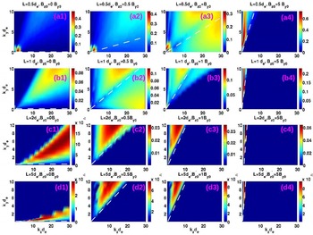
Growth rates in
 $k_{y}$
–
 $k_{z}$
space for various values of
 $L$
and
 $B_{z0}$
are shown in figure 2. In general, the modes with
 $kd_{e}\sim 1$
and/or
 $kd_{e}\gg 1$
have finite growth rates in select regions of
 $k_{y}$
–
 $k_{z}$
space. For example, in the panel for
 $L/d_{e}=0.5$
and
 $B_{z0}=B_{y0}$
, unstable modes can be seen in the bottom-left (
 $kd_{e}\sim 1$
) and top-right (
 $kd_{e}\gg 1$
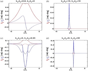
) corners of the panel. The eigenfunctions of the select modes chosen from the two corners of the panel are shown in figure 3. The typical signature of tearing mode can be seen in the eigenfunctions for
 $k_{y}d_{e}=0.8$
and
 $k_{z}d_{e}=0$
, figure 3. In fact, the 2-D modes with
 $k_{z}=0$
are always tearing modes and are not affected by the guide field. The eigenfunctions in the other three panels, figure 3(b–d), are different from tearing eigenfunctions. Although the mode with
 $k_{y}d_{e}=10$
and
 $k_{z}d_{e}=16$
, figure 3(b), falls in the region (above the white dashed line) of the
 $k_{y}$
–
 $k_{z}$
space where a mode rational surface exists, it is not a tearing mode. This is because the existence of mode rational surfaces is only a necessary condition for the tearing mode. The modes in figure 3(c) (
 $k_{y}d_{e}=0$
and
 $k_{z}d_{e}=2.25$
) and figure 3(d) (
 $k_{y}d_{e}=8$
and
 $k_{z}d_{e}=30$
) fall in the region of
 $k_{y}$
–
 $k_{z}$
space where mode resonance surfaces do not exist. This indicates that tearing modes exist only for very small values of
 $k_{z}$
when
 $0<k_{y}L<1$
for given values of
 $L$
and
 $B_{z0}$
.
Growth rates
 ${\it\gamma}/{\it\omega}_{ce}$
(colour) of ESFI in
 $k_{y}$
–
 $k_{z}$
space for
 $L/d_{e}=0.5$
, 1.0, 2.0 and 5.0 (along column). For each value of
 $L$
,
 $B_{z0}/B_{y0}=0$
, 0.5, 1.0 and 5.0. (along row). White dashed lines separate the regions of the existence (on the left or above the line) and non-existence (on the right or below the line) of mode rational surfaces according to the (3.5) and (3.6).

Real (solid) and imaginary (dashed) parts of eigenfunctions
 $v_{x}$
(blue) and
 $b_{x}$
(red) for various values of
 $k_{y}$
and
 $k_{z}$
when
 $L=0.5\,d_{e}$
and
 $B_{z0}=B_{y0}$
.

One distinctive feature of non-tearing modes is the even parity of
 $v_{x}$
in contrast to its odd parity for the tearing mode. Also, eigenfunctions become increasingly localized with increasing
 $k$
. In the limit of large
 $k$
, the first term on the right-hand side of (2.2) can be neglected (Jain & Büchner Reference Jain and Büchner2014a
). This gives us an equations for
 $v_{x}$
.
 $$\begin{eqnarray}\displaystyle d_{e}^{2}\frac{\text{d}^{2}v_{x}}{\text{d}x^{2}}-\left[1+k^{2}d_{e}^{2}-\frac{d_{e}^{2}{\it\omega}_{ce}^{2}}{B_{y0}^{2}}\frac{F(F-d_{e}^{2}F^{\prime \prime })}{\bar{{\it\omega}}^{2}}+\frac{k_{z}(v_{0}-d_{e}^{2}v_{0}^{\prime \prime })}{\bar{{\it\omega}}}\right]v_{x}=0. & & \displaystyle\end{eqnarray}$$
As
 $k$
increases, the decay length of the solution of (3.9) decreases and thus the eigenfunctions become increasingly localized. For non-tearing modes,
 $b_{x}<v_{x}$
which holds stronger as
 $k$
increases. This can be seen from (2.3) by comparing the left-hand side and right-hand side, giving,
 $$\begin{eqnarray}\displaystyle \frac{b_{x}}{v_{x}}=-\frac{F-d_{e}^{2}F^{\prime \prime }}{\bar{{\it\omega}}(1+k^{2}d_{e}^{2}+k_{x}^{2}d_{e}^{2})}, & & \displaystyle\end{eqnarray}$$
where
 $k_{x}^{-1}$
is the
 $x$
-scale length of the eigenfunctions. It is clear from (3.10) that the ratio
 $b_{x}/v_{x}$
drops as
 $k$
increases.
The effect of guide field can be understood by noting that the guide field appears in (2.2) and (2.3) through the terms involving
 $F=k_{z}B_{z0}+k_{y}B_{0}(x)$
and
 $F-d_{e}^{2}F^{\prime \prime }=k_{z}B_{z0}+k_{y}B_{0}(x)+k_{y}d_{e}^{2}v_{0}^{\prime }(x)$
, where
 $B_{0}(x)={\hat{y}}\boldsymbol{\cdot }\boldsymbol{B}_{0}$
. For
 $L\ll d_{e}$
,
 $d_{e}^{2}v_{0}^{\prime }\sim d_{e}^{2}B_{y0}/L^{2}\gg B_{y0}$
resulting in
 $F-d_{e}^{2}F^{\prime \prime }\approx k_{y}v_{0}^{\prime }+k_{z}B_{z0}$
. In the opposite limit
 $L\gg d_{e}$
,
 $d_{e}^{2}v_{0}^{\prime }\sim d_{e}^{2}B_{y0}/L^{2}\ll B_{y0}$
and
 $F-d_{e}^{2}F^{\prime \prime }\approx k_{y}B_{0}+k_{z}B_{z0}$
. Thus the conditions under which the guide field affects the growth rate can be stated as follows.
 $$\begin{eqnarray}\displaystyle & \displaystyle \frac{k_{y}}{k_{z}}\lesssim \frac{L^{2}}{d_{e}^{2}}\,\frac{B_{z0}}{B_{y0}},\quad L\ll d_{e} & \displaystyle\end{eqnarray}$$
 $$\begin{eqnarray}\displaystyle & \displaystyle \frac{k_{y}}{k_{z}}\lesssim \frac{B_{z0}}{B_{y0}},\quad L\gg d_{e}. & \displaystyle\end{eqnarray}$$
These conditions are similar to the conditions for the non-existence of the tearing mode given by (3.5) and (3.6). Thus, for given values of
 $L$
and
 $B_{z0}$
, the guide field affects the modes in the select region of
 $k_{y}{-}k_{z}$
space given by (3.11) and (3.12). For the modes with
 $k_{y}/k_{z}\ll B_{z0}/B_{y0}$
(for
 $L\gg d_{e}$
) or
 $k_{y}/k_{z}\ll (L^{2}/d_{e}^{2})(B_{z0}/B_{y0})$
(for
 $L\ll d_{e}$
), the guide field term dominates and
 $F=F-d_{e}^{2}F^{\prime \prime }=k_{z}B_{z0}$
. These modes can be unstable for
 $L\lesssim d_{e}$
as the term
 $\propto d_{e}^{2}v_{0}^{\prime \prime }\sim d_{e}^{2}v_{0}/L^{2}\gtrsim v_{0}$
(the only term left causing the instability) survives in the last term on the right-hand side of (2.2). For
 $L\gg d_{e}$
, these modes are stable as the term
 $\propto d_{e}^{2}v_{0}^{\prime \prime }\sim d_{e}^{2}v_{0}/L^{2}\ll v_{0}$
can be neglected.
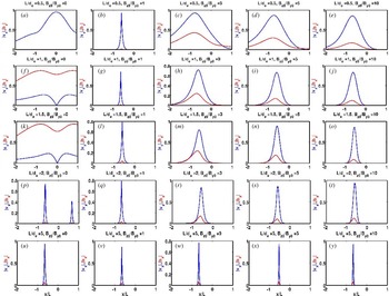
These effects of the guide field can be seen in figure 2. For
 $L>d_{e}$
, the growth rate is zero in the region where
 $k_{y}/k_{z}\ll B_{z0}/B_{y0}$
(below white dashed line). As a consequence, the domain of the unstable modes shifts to smaller values of
 $k_{z}$
as the strength of the guide field increases for a fixed
 $L$
. For
 $L<d_{e}$
, e.g.
 $L=0.5\,d_{e}$
and
 $B_{z0}=B_{y0}$
in figure 2, the modes with
 $k_{y}/k_{z}\lesssim (L^{2}/d_{e}^{2})(B_{z0}/B_{y0})=0.25$
(below and around the white dashed line) have finite growth rates. That is why panels (a3) and (b2) look different from the other panels in figure 2.
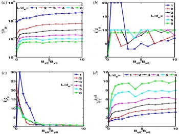
Growth rates
 ${\it\gamma}_{f}$
(a), wavenumbers
 $k_{y}^{f}$
(b) and
 $k_{z}^{f}$
(c) of the fastest growing mode as functions of guide field
 $B_{z0}$
for various current sheet thicknesses. In (d), ratio
 ${\it\gamma}_{f}/{\it\gamma}_{f}^{k_{z}=0}$
, where
 ${\it\gamma}_{f}^{k_{z}=0}$
is the growth rate of the fastest 2-D (
 $k_{z}=0$
) tearing mode as a function of the guide field.

The maximum growth rate drops rapidly with
 $L$
for a given value of the guide field, but increases slowly with the guide field for fixed current sheet thickness. An electron shear flow instability whose growth rate increases with the strength of the guide field was also reported in 3-D PIC simulations of electron current sheets (Che et al.
Reference Che, Drake and Swisdak2011). The variation of the growth rate (
 ${\it\gamma}_{f}$
) of the fastest growing mode (maximum growth rate in
 $k_{y}$
–
 $k_{z}$
space) with the strength of the guide field for various values of
 $L$
is shown in figure 4(a). The rate of increase of the growth rate with the guide field is faster for weak guide field (
 $B_{z0}/B_{y0}<1$
) as compared to the rate for strong guide field (
 $B_{z0}/B_{y0}>5$
). In between the fast and slow rise of the growth rate with the guide field, a plateau forms. The rate of the fast rise of
 ${\it\gamma}_{f}$
(for weak guide field) increases with
 $L$
, while the rate of the slow rise (for strong guide field) decreases with
 $L$
. The range of the guide field values for the plateau depends on
 $L$
.
The wavenumbers,
 $k_{y}^{f}$
and
 $k_{z}^{f}$
, of the fastest growing mode are shown in figure 4(b,c). The wavenumber
 $k_{y}^{f}$
makes a jump to large values as soon as the guide field becomes finite, and remains at this value for a range of the values of guide field. On further increasing the guide field,
 $k_{y}^{f}$
drops and then rises again. This trend of variation of
 $k_{y}^{f}$
with the guide field can be seen for all values of
 $L$
. The jump in the value of
 $k_{y}^{f}$
is largest for
 $L=d_{e}$
. The wavenumber
 $k_{z}^{f}$
has a large jump as soon as the guide field becomes finite only for
 $L=d_{e}$
. After the initial jump,
 $k_{z}^{f}$
drops. For
 $L>d_{e}$
,
 $k_{z}^{f}$
drops with increasing guide field. For all values of
 $L$
,
 $k_{z}^{f}$
saturates at
 $k_{z}^{f}d_{e}\approx 1$
for large values of guide field. The sudden changes in
 ${\it\gamma}_{f}$
,
 $k_{y}^{f}$
and
 $k_{z}^{f}$
as soon as the guide field becomes finite indicate that the inclusion of the guide field triggers a new kind of unstable mode, different from the tearing mode.
The eigenfunctions
 $v_{x}$
and
 $b_{x}$
obtained from (2.2) and (2.3) are, in general, complex and contain phase and magnitude information in their real and imaginary parts. The physical electron velocity (
 $V_{x}$
) and magnetic field (
 $B_{x}$
) perturbations are related to the complex eigenfunctions,
 $v_{x}(x)=|v_{x}|\exp (\text{i}{\it\theta}_{v})$
and
 $b_{x}(x)=|b_{x}|\exp (\text{i}{\it\theta}_{b})$
, as
 $V_{x}=\text{Re}[v_{x}(x)\text{e}^{\text{i}(k_{y}y+k_{z}z-{\it\omega}t)}]$
and
 $B_{x}=\text{Re}[b_{x}(x)\text{e}^{\text{i}(k_{y}y+k_{z}z-{\it\omega}t)}]$
. Here
 $|v_{x}|^{2}=[\text{Re}(v_{x})]^{2}+[\text{Im}(v_{x})]^{2}$
,
 $|b_{x}|^{2}=[\text{Re}(b_{x})]^{2}+[\text{Im}(b_{x})]^{2}$
,
 $\tan ({\it\theta}_{v})=\text{Im}(v_{x})/\text{Re}(v_{x})$
and
 $\tan ({\it\theta}_{b})=\text{Im}(b_{x})/\text{Re}(b_{x})$
. Substituting for
 $v_{x}$
and
 $b_{x}$
relates the physical variables
 $V_{x}$
and
 $B_{x}$
to the absolute values
 $|v_{x}|$
and
 $|b_{x}|$
which, for the fastest mode, are plotted in figure 5 in order to distinguish between tearing and non-tearing modes.
Absolute values of complex eigenfunctions
 $v_{x}$
(blue) and
 $b_{x}$
(red) corresponding to the fastest growing mode for
 $L/d_{e}=0.5,1,1.5,2$
and 5 (varying along a column), and
 $B_{z0}/B_{y0}=0,1,3,5$
and 10 (varying along a row). Horizontal axis is in units of
 $L$
and shows only a small region in
 $x$
.

For the tearing mode, the
 $x$
-component of the physical magnetic field (
 $B_{x}$
) and velocity (
 $V_{x}$
) should be finite and zero, respectively, at the mode rational surface. In figure 5, panels for
 $B_{z0}=0$
,
 $L/d_{e}=1$
( f) and
 $B_{z0}=0,L/d_{e}=1.5$
(k) show the typical signature of the tearing mode, namely,
 $|v_{x}|=0$
and
 $|b_{x}|\neq 0$
(therefore also for
 $V_{x}$
and
 $B_{x}$
) at the same location
 $x=0$
(mode resonance surface). No other panel shows the simultaneous occurrence of
 $|v_{x}|=0$
and
 $|b_{x}|\neq 0$
at a mode resonance surface. Therefore, the tearing mode is the fastest growing mode in a very small range (around
 $L=d_{e}$
and
 $B_{z0}=0$
) of
 $L{-}B_{z0}$
parameter space.
Although the fastest growing mode is non-tearing in the presence of a finite guide field, the 2-D tearing mode (
 $k_{z}=0$
) is not affected by the guide field because the guide field disappears from (2.2) and (2.3) for
 $k_{z}=0$
. For
 $L=d_{e}$
and
 $B_{z0}=B_{y0}$
, the growth rate of the fastest 2-D tearing mode (
 $k_{y}d_{e}=0.4$
) is comparable to that of the fastest growing 3-D non-tearing mode (figure 2). In order to determine the relative importance of the tearing and non-tearing modes as a function of
 $L$
and
 $B_{z0}$
, we compare the growth rate of the fastest 3-D mode (
 ${\it\gamma}_{f}$
) and that of the fastest 2-D (
 $k_{z}=0$
) tearing mode (
 ${\it\gamma}_{f}^{k_{z}=0}$
) in figure 4(d). The ratio
 ${\it\gamma}_{f}/{\it\gamma}_{f}^{k_{z}=0}$
increases with both the current sheet thickness and the strength of the guide field. For zero guide field, the ratio
 ${\it\gamma}_{f}/{\it\gamma}_{f}^{k_{z}=0}$
is of the order of unity (varies from 1 to 3 for
 $L/d_{e}=1$
to 6). The ratio increases with the strength of the guide field but remains of order unity for thinner current sheets (
 $L/d_{e}=1$
and 2) for guide fields as large as
 $B_{z0}/B_{y0}=10$
. The initial rate of increase of the ratio with guide field is larger for thicker current sheets. Therefore the ratio increases to much larger values even for
 $L>2\,d_{e}$
. It is expected that the tearing mode can grow simultaneously with the non-tearing modes for thin current sheets and small values of guide field.
4. Conclusion and discussion
Our results obtained in the limit of
 ${\it\beta}_{e}\ll 1$
from eigenvalue analysis of linear EMHD equations show that the conditions under which an ECS is unstable to tearing or non-tearing mode depends on the thickness of ECS, strength of the guide field and the wavenumber of the mode. The fastest growing mode is the 2-D (
 $k_{z}=0$
) tearing mode for current sheet thicknesses
 $1\leqslant L/d_{e}\leqslant 1.5$
and a very weak guide field
 $B_{z0}\approx 0$
. For all other values of
 $L$
and
 $B_{z0}$
, the non-tearing mode is the fastest growing. The growth rate of the fastest mode drops rapidly with current sheet thickness but increases slowly with the strength of the guide field. The wavenumber
 $k_{z}^{f}$
(along the direction of guide field) of the fastest growing non-tearing mode drops with the strength of the guide field. For current sheet thicknesses
 $L/d_{e}=1{-}6$
(considered in this paper), it is
 $k_{z}^{f}d_{e}\gg 1$
for
 $B_{z0}/B_{y0}\approx 1$
and drops to saturate at
 $k_{z}^{f}d_{e}\approx 1$
for guide fields above
 $B_{z0}/B_{y0}\approx 4$
. Thus the non-tearing instability remains 3-D for large guide fields.
A general mode resonance condition,
 $\boldsymbol{k}\boldsymbol{\cdot }(\boldsymbol{B}_{0}-d_{e}^{2}\boldsymbol{B}_{0}^{\prime \prime })$
, for the EMHD tearing mode was obtained. It was shown that the general resonance condition for the MHD tearing mode,
 $\boldsymbol{k}\boldsymbol{\cdot }(\boldsymbol{B}_{0}-L_{{\it\eta}}^{2}\boldsymbol{B}_{0}^{\prime \prime })$
, is different from the usual resonance condition
 $\boldsymbol{k}\boldsymbol{\cdot }\boldsymbol{B}_{0}=0$
. However, the general resonance condition for the EMHD (MHD) tearing mode reduces to
 $\boldsymbol{k}\boldsymbol{\cdot }\boldsymbol{B}_{0}=0$
if the equilibrium scale length is much larger than the electron inertial length (resistive scale length). The conditions for the non-existence of the tearing mode were obtained. These conditions relate wavenumbers, current sheet thickness and strength of the guide field.
Our results obtained by eigenvalue analysis of linear EMHD equations are consistent with the 2-D and 3-D PIC simulations of (Che et al.
Reference Che, Drake and Swisdak2011; Liu et al.
Reference Liu, Daughton, Karimabadi, Li and Roytershteyn2013), which show the growth of tearing and/or non-tearing instabilities in force-free electron current sheets depending upon the thickness of the sheet, strength of the guide field and available domain of unstable wavenumbers. In the limit of large guide field, the force-free electron current sheet is similar to the equilibrium electron current sheet in our studies. We shall discuss these PIC simulations (Che et al.
Reference Che, Drake and Swisdak2011; Liu et al.
Reference Liu, Daughton, Karimabadi, Li and Roytershteyn2013) in the coordinate system used to define the equilibrium (
 $\boldsymbol{B}_{0}=B_{y0}\tanh (x/L){\hat{y}}+B_{z0}\hat{z}$
) in this paper.
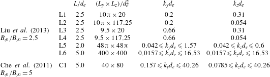
Parameters of PIC simulations of Liu et al. (Reference Liu, Daughton, Karimabadi, Li and Roytershteyn2013) and Che et al. (Reference Che, Drake and Swisdak2011).

Table 1 summarizes the 3-D PIC simulation parameters (relevant for our discussion) of Che et al. (Reference Che, Drake and Swisdak2011) and Liu et al. (Reference Liu, Daughton, Karimabadi, Li and Roytershteyn2013). The six simulations of Liu et al. are named L1–L6 while C1 is a single simulation of Che et al. The results of simulations L1, L2, L5 and L6 are shown in figures 2(a–c) and 3 of Liu et al. (Reference Liu, Daughton, Karimabadi, Li and Roytershteyn2013), respectively. Simulations L3 and L4 were carried out for the same parameters as L1 and L2, respectively, except for
 $L_{y}=3.8\,L$
. The wavenumbers for simulations L1–L4 are calculated as
 $k_{y}d_{e}=2{\rm\pi}/L_{y}$
and
 $k_{z}d_{e}=2{\rm\pi}/L_{z}$
(
 $L_{y}$
and
 $L_{z}$
are the simulation box sizes along the
 $y$
and
 $z$
directions, respectively) corresponding to the initial perturbation added to the equilibrium in the PIC simulations. Note that the simulations L1–L4 also contain wavemodes with higher wavenumbers, however, initialized modes dominate the evolution. The lower bounds of the range of the values of
 $k_{y}$
and
 $k_{z}$
for simulation L5 are calculated as
 $k_{y,z}^{min}=2{\rm\pi}/L_{y,z}$
while upper bounds are read from figure 2(c) of Liu et al. (Reference Liu, Daughton, Karimabadi, Li and Roytershteyn2013), assuming that it shows the fluctuation spectrum for the whole range of wavenumbers in the simulation. The wavenumber range for simulations L6 and C1 are obtained by calculating the minimum and maximum wavenumbers (
 $k_{y,z}^{min}=2{\rm\pi}/L_{y,z}$
and
 $k_{y,z}^{max}={\rm\pi}/{\it\Delta}_{y,z}$
, where
 ${\it\Delta}_{y,z}$
are the grid resolutions) present in these simulations.
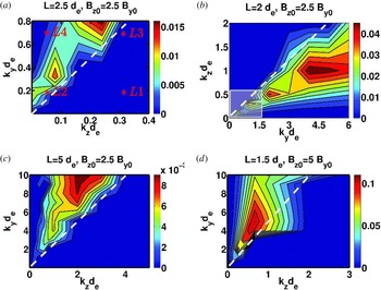
Simulations L1–L4 are marked by ‘
 $\ast$
’ in the wavenumber space in figure 6(a) which shows that the initialized mode for simulations L1, L3 and L4 are stable while it is tearing unstable for L2. In the case of L1, the unstable tearing mode with
 $k_{y}d_{e}=0.2$
but
 $k_{z}=0$
will grow in the simulations. This is consistent with the results of Liu et al. (Reference Liu, Daughton, Karimabadi, Li and Roytershteyn2013), which show growth of the tearing mode for L1 and L2 and no growth for L3 and L4. The range of wavenumbers covered in simulation L5 is enclosed by the white rectangle in figure 6(b). The fluctuations in L5 have finite power, corresponding to the unstable modes inside the rectangle (compare with figure 2c of Liu et al. (Reference Liu, Daughton, Karimabadi, Li and Roytershteyn2013)). In order to facilitate the comparison with figure 2(c) of Liu et al., the horizontal (
 $k_{y}d_{e}$
) and vertical (
 $k_{z}d_{e}$
) axes in figure 6(b) are interchanged. Note that simulation L5 does not include the faster growing modes (non-tearing) with larger values of
 $k_{y}d_{e}$
and
 $k_{z}d_{e}$
(see figure 6
b). However, simulation L6 covers an extensive range of wavenumbers and does include the fastest growing mode. The electron current sheets formed in L6 are at an angle of 11°, i.e.
 $k_{z}/k_{y}=\tan (11^{\circ })\approx 0.19$
. From the growth rate plot for the parameters of L6, figure 6(c), we find that
 $k_{z}/k_{y}\approx 2/10=0.2$
for the fastest growing mode, in close agreement with the simulation results.
Linear growth rates
 ${\it\gamma}/{\it\omega}_{ce}$
of ESFIs in wavevector space for the PIC simulation parameters of Che et al. (Reference Che, Drake and Swisdak2011) and Liu et al. (Reference Liu, Daughton, Karimabadi, Li and Roytershteyn2013). In (a), stars ‘
 $\ast$
’ labelled L1–L4 correspond to the PIC simulations L1–L4 listed in table 1. White dashed lines separate the regions of the existence (on the left or above the line) and non-existence (on the right or below the line) of mode rational surfaces according to the (3.5) and (3.6). Note that the horizontal and vertical axes in (b) are
 $k_{y}d_{e}$
and
 $k_{z}d_{e}$
, respectively, different from those in (a), (c) and (d).

In addition, Liu et al. (Reference Liu, Daughton, Karimabadi, Li and Roytershteyn2013) carried out 2-D PIC simulations in
 $x^{\prime }$
–
 $y^{\prime }$
planes rotated about the
 $x$
-axis by an angle
 ${\it\theta}$
. The wavenumber
 $k_{y}^{\prime }$
in the rotated coordinate system is related to
 $k_{y}$
and
 $k_{z}$
as
 $k_{z}=k_{y^{\prime }}\sin ({\it\theta})$
and
 $k_{y}=k_{y^{\prime }}\cos ({\it\theta})$
. For
 $0\leqslant {\it\theta}\leqslant 90^{\circ }$
and fixed
 $k_{y^{\prime }}L=0.5$
considered by Liu et al. (Reference Liu, Daughton, Karimabadi, Li and Roytershteyn2013),
 $0\leqslant k_{y}L$
,
 $k_{z}L\leqslant 0.5$
. For this range of
 $k_{y}$
and
 $k_{z}$
, the tearing mode is dominant (figure 2), consistent with the 2-D PIC simulations (Liu et al.
Reference Liu, Daughton, Karimabadi, Li and Roytershteyn2013).
Reconnection in the 3-D simulation C1 (Che et al.
Reference Che, Drake and Swisdak2011), which covers a wide range of wavenumbers, is initiated with a large-scale magnetic perturbation. The half-thickness of the force-free electron current sheet reduces from its initial value
 $L=5\,d_{e}$
to
 $L\approx 1.5\,d_{e}$
until the onset of the current filamentation instability at
 ${\it\omega}_{ci}t\approx 3.3$
. As a result of the instability, the current sheet broadens to have
 $L\approx 2\,d_{e}$
by
 ${\it\omega}_{ci}t=3.75$
. The evolution of the instability between
 ${\it\omega}_{ci}t\approx 3.3{-}3.5$
can be considered to be in the linear phase during which the half-thickness is not changing (see figure 1a of Che et al.
Reference Che, Drake and Swisdak2011). The growth rate of the filamentation instability in simulation C1 can be estimated from the linear phase as
 ${\it\gamma}^{che}/{\it\omega}_{ce}\approx 0.05$
(mass ratio
 $m_{i}/m_{e}=100$
in C1). The fastest growing mode for
 $L=1.5\,d_{e}$
and
 $B_{z0}=5\,B_{y0}$
, figure 6(d), has
 ${\it\gamma}^{f}\approx 0.1{\it\omega}_{ce}\sim {\it\gamma}^{che}$
and
 $k_{z}^{f}d_{e}\approx 0.65$
, giving wavelength
 ${\it\lambda}_{z}\approx 10d_{e}$
of the same order of magnitude as the length of the filaments in figure 3(b) of Che et al. (Reference Che, Drake and Swisdak2011).
Although the tearing modes are not the fastest growing mode, they may grow slowly and play an important role later in the nonlinear stage of the evolution of the electron current sheet. Our linear results have been obtained for an undriven electron current sheet. However, in cases where reconnection is driven from boundaries such as in laboratory experiments (Dorfman et al. Reference Dorfman, Ji, Yamada, Yoo, Lawrence, Myers and Tharp2013; Bohlin et al. Reference Bohlin, Stechow, Rahbarnia, Grulke and Klinger2014), the evolution of the current sheet may be dominated by the tearing mode even for large guide field and thicker current sheets.
Acknowledgements
This work was supported by Max-Planck/Princeton Center for Plasma Physics at the Max Planck Institute for Solar System Research, Justus-von-Liebig-Weg-3, Göttingen, Germany. One of the authors (J.B.) gratefully acknowledges the support of the German Science Foundation CRC 963 for this work. We thank Dr B. Bandow for his help to numerically optimize the EMHD code.