2.1 Particle number density function

Let $f_{p}(\boldsymbol{x},\boldsymbol{c}_{p},q_{p},t)$ denote the number density function of particles at position $\boldsymbol{x}$ with velocity $\boldsymbol{c}_{p}$ and charge $q_{p}$ . Hence, the number of particles with velocity between $\boldsymbol{c}_{p}$ and $\boldsymbol{c}_{p}+\text{d}\boldsymbol{c}_{p}$ and charge between $q_{p}$ and $q_{p}+\text{d}q_{p}$ at position $\boldsymbol{x}$ and time $t$ is given by $f_{p}\,\text{d}\boldsymbol{c}_{p}\,\text{d}q_{p}$ . The evolution of the particle number density function follows the Boltzmann equation:

(2.1) $$\begin{eqnarray}\displaystyle \frac{\unicode[STIX]{x2202}f_{p}}{\unicode[STIX]{x2202}t}+\frac{\unicode[STIX]{x2202}}{\unicode[STIX]{x2202}x_{j}}(c_{p,j}f_{p})+\frac{\unicode[STIX]{x2202}}{\unicode[STIX]{x2202}c_{p,j}}\left(\left\langle \left.\frac{\text{d}c_{p,j}}{\text{d}t}\right|\boldsymbol{c}_{p},q_{p}\right\rangle f_{p}\right)+\frac{\unicode[STIX]{x2202}}{\unicode[STIX]{x2202}\unicode[STIX]{x1D701}_{p}}\left(\left\langle \left.\frac{\text{d}q_{p}}{\text{d}t}\right|\boldsymbol{c}_{p},q_{p}\right\rangle f_{p}\right)=\left(\frac{\unicode[STIX]{x2202}f_{p}}{\unicode[STIX]{x2202}t}\right)_{coll}, & & \displaystyle \nonumber\\ \displaystyle & & \displaystyle\end{eqnarray}$$

where $\text{d}/\text{d}t$ is the rate of any particle property change along the particle path due to the exchange with the fluid and the influence of resolved fields. The notation $\langle {\mathcal{G}}|\boldsymbol{c}_{p},q_{p}\rangle$ is the expected value $\langle {\mathcal{G}}|c_{p,j}={\mathcal{C}}_{p,j},q_{p}={\mathcal{q}}_{p}\rangle$ , and $(\unicode[STIX]{x2202}f_{p}/\unicode[STIX]{x2202}t)_{coll}$ is the rate of distribution function change due to particle–particle interactions.

2.2 Discrete particle equations

The Lagrangian approach provides a direct description of discrete phases by tracking particles of the system. By following Gatignol (Reference Gatignol1983) and Maxey (Reference Maxey1983), the equation of motion for an isolated particle can be written as

(2.2) $$\begin{eqnarray}m_{p}\frac{\text{d}c_{p,i}}{\text{d}t}=-V_{p}\frac{\unicode[STIX]{x2202}p_{g}}{\unicode[STIX]{x2202}x_{i}}+m_{p}g_{i}-\frac{m_{p}}{\unicode[STIX]{x1D70F}_{p}^{\ast }}(c_{p,i}-u_{g,i})+F_{e,i},\end{eqnarray}$$

where the first term is the instantaneous undisturbed pressure gradient at the particle centre (Archimedes force) and $g_{i}$ is the acceleration due to gravity in the $i$ th direction. The third term represents the fluid–particle drag force. In (2.2), $m_{p}=\unicode[STIX]{x1D70C}_{p}V_{p}$ is the mass of a particle, $\unicode[STIX]{x1D70C}_{p}$ is the particle density, $V_{p}$ is the particle volume and $u_{g,i}$ is the gas velocity of the undisturbed flow. The relaxation time of a single particle $\unicode[STIX]{x1D70F}_{p}^{\ast }$ is given by

(2.3) $$\begin{eqnarray}\displaystyle \frac{1}{\unicode[STIX]{x1D70F}_{p}^{\ast }}=\frac{3}{4}\frac{\unicode[STIX]{x1D70C}_{g}}{\unicode[STIX]{x1D70C}_{p}}\frac{C_{D}}{d_{p}}|\boldsymbol{c}_{p}-\boldsymbol{u}_{g}|, & & \displaystyle\end{eqnarray}$$

where $\unicode[STIX]{x1D70C}_{g}$ is the fluid density, $C_{D}$ is the drag coefficient, given by Schiller & Naumann (Reference Schiller and Naumann1935) as

(2.4) $$\begin{eqnarray}C_{D}=\frac{24}{Re_{p}}(1+0.15\,Re_{p}^{0.687}),\end{eqnarray}$$

where

(2.5) $$\begin{eqnarray}Re_{p}=\frac{|\boldsymbol{c}_{p}-\boldsymbol{u}_{g}|d_{p}}{\unicode[STIX]{x1D708}_{g}}\end{eqnarray}$$

with $\unicode[STIX]{x1D708}_{g}$ the kinematic viscosity of the gas and $d_{p}$ the particle diameter. Here $F_{e,i}$ is the electrostatic force, which is given by

(2.6) $$\begin{eqnarray}F_{e,i}=q_{p}\,E_{i},\end{eqnarray}$$

where $E_{i}$ is the resolved electric field and dielectrophoretic forces are neglected (LaMarche et al. Reference LaMarche, Muzzio, Shinbrot and Glasser2010). The resolved electric field is computed by solving a Poisson equation

(2.7) $$\begin{eqnarray}\unicode[STIX]{x1D6FB}^{2}\unicode[STIX]{x1D719}=-\frac{\unicode[STIX]{x1D70C}}{\unicode[STIX]{x1D716}}\end{eqnarray}$$

for the electrical potential $\unicode[STIX]{x1D719}$ , where $\unicode[STIX]{x1D70C}$ is the charge density and $\unicode[STIX]{x1D716}$ is the (mixture) electrical permittivity. Then, the resolved electric field is obtained by taking the gradient of the electrical potential $\unicode[STIX]{x1D719}$ :

(2.8) $$\begin{eqnarray}E_{i}=-\unicode[STIX]{x1D735}\unicode[STIX]{x1D719}.\end{eqnarray}$$

2.3 Particle moment equations

The dispersed phase average of any function $\unicode[STIX]{x1D713}(\boldsymbol{c}_{p},q_{p})$ can be obtained by integrating over the particle property space as

(2.9) $$\begin{eqnarray}\langle \unicode[STIX]{x1D713}\rangle =\frac{1}{n_{p}}\int _{\mathbb{R}^{3}}\int _{\mathbb{R}}\unicode[STIX]{x1D713}f_{p}\,\text{d}q_{p}\,\text{d}\boldsymbol{c}_{p},\end{eqnarray}$$

where $n_{p}$ is the mean number of particles per unit volume, or namely particle number density given by

(2.10) $$\begin{eqnarray}n_{p}(\boldsymbol{x},t)=\int _{\mathbb{R}^{3}}\int _{\mathbb{R}}f_{p}\,\text{d}q_{p}\,\text{d}\boldsymbol{c}_{p}.\end{eqnarray}$$

By definition, the mean velocity of particles is

(2.11) $$\begin{eqnarray}U_{p,i}=\langle c_{p,i}\rangle =\frac{1}{n_{p}}\int _{\mathbb{R}^{3}}\int _{\mathbb{R}}c_{p,i}f_{p}\,\text{d}\boldsymbol{c}_{p}\,\text{d}q_{p}\end{eqnarray}$$

and the fluctuating part of the disperse phase velocity is

(2.12) $$\begin{eqnarray}c_{p,i}^{\prime }=c_{p,i}-U_{p,i}.\end{eqnarray}$$

The particle kinetic tensor is given by

(2.13) $$\begin{eqnarray}\langle c_{p,i}^{\prime }c_{p,j}^{\prime }\rangle =\frac{1}{n_{p}}\int _{\mathbb{R}^{3}}\int _{\mathbb{R}}(c_{p,i}-U_{p,i})(c_{p,j}-U_{p,j})f_{p}\,\text{d}\boldsymbol{c}_{p}\,\text{d}q_{p}.\end{eqnarray}$$

The mean particle charge is

(2.14) $$\begin{eqnarray}Q_{p}=\langle q_{p}\rangle =\frac{1}{n_{p}}\int _{\mathbb{R}^{3}}\int _{\mathbb{R}}q_{p}f_{p}\,\text{d}\boldsymbol{c}_{p}\,\text{d}q_{p}\end{eqnarray}$$

and the fluctuating part of the phase charge is

(2.15) $$\begin{eqnarray}q_{p}^{\prime }=q_{p}-Q_{p}.\end{eqnarray}$$

The charge variance is then given by

(2.16) $$\begin{eqnarray}\langle q_{p}^{\prime }q_{p}^{\prime }\rangle =\frac{1}{n_{p}}\int _{\mathbb{R}^{3}}\int _{\mathbb{R}}(q_{p}-Q_{p})^{2}f_{p}\,\text{d}\boldsymbol{c}_{p}\,\text{d}q_{p}.\end{eqnarray}$$

The correlations between the velocity fluctuations and the charge fluctuation are defined as

(2.17) $$\begin{eqnarray}\langle q_{p}^{\prime }c_{p,i}^{\prime }\rangle =\frac{1}{n_{p}}\int _{\mathbb{R}^{3}}\int _{\mathbb{R}}(q_{p}-Q_{p})(c_{p,i}-U_{p,i})f_{p}\,\text{d}\boldsymbol{c}_{p}\,\text{d}q_{p}.\end{eqnarray}$$

Enskog’s general equation for the change of a function $\unicode[STIX]{x1D713}(\boldsymbol{c}_{p},q_{p})$ can be derived from the transport equation of the number density function (2.1) by integrating over the particle property space and using the relation $n_{p}\,m_{p}=\unicode[STIX]{x1D6FC}_{p}\unicode[STIX]{x1D70C}_{p}$ , where $\unicode[STIX]{x1D6FC}_{p}$ is the solid phase volume fraction, as

(2.18) $$\begin{eqnarray}\frac{\unicode[STIX]{x2202}}{\unicode[STIX]{x2202}t}(\unicode[STIX]{x1D6FC}_{p}\unicode[STIX]{x1D70C}_{p}\langle \unicode[STIX]{x1D713}\rangle )+\frac{\unicode[STIX]{x2202}}{\unicode[STIX]{x2202}x_{i}}(\unicode[STIX]{x1D6FC}_{p}\unicode[STIX]{x1D70C}_{p}\langle c_{p,i}\unicode[STIX]{x1D713}\rangle )={\mathcal{C}}(m_{p}\unicode[STIX]{x1D713})+\unicode[STIX]{x1D6FC}_{p}\unicode[STIX]{x1D70C}_{p}\left\langle \frac{\text{d}c_{p,i}}{\text{d}t}\frac{\unicode[STIX]{x2202}\unicode[STIX]{x1D713}}{\unicode[STIX]{x2202}c_{p,i}}\right\rangle +\unicode[STIX]{x1D6FC}_{p}\unicode[STIX]{x1D70C}_{p}\left\langle \frac{\text{d}q_{p}}{\text{d}t}\frac{\unicode[STIX]{x2202}\unicode[STIX]{x1D713}}{\unicode[STIX]{x2202}q_{p}}\right\rangle .\end{eqnarray}$$

The mean collisional rate of change of the particle property ${\mathcal{C}}(m_{p}\unicode[STIX]{x1D713})$ is the change of $(m_{p}\unicode[STIX]{x1D713})$ due to all collisions. The particle charge is not changed by the resolved field except during the contact. Thus,

(2.19) $$\begin{eqnarray}\displaystyle \frac{\text{d}q_{p}}{\text{d}t}=0 & & \displaystyle\end{eqnarray}$$

and the last term in (2.18) drops outs.

2.4 Mass balance $(\unicode[STIX]{x1D713}=1)$

The mass balance equation for the solid phase is given by

(2.20) $$\begin{eqnarray}\frac{\unicode[STIX]{x2202}}{\unicode[STIX]{x2202}t}(\unicode[STIX]{x1D6FC}_{p}\unicode[STIX]{x1D70C}_{p})+\frac{\unicode[STIX]{x2202}}{\unicode[STIX]{x2202}x_{i}}(\unicode[STIX]{x1D6FC}_{p}\unicode[STIX]{x1D70C}_{p}U_{p,i})={\mathcal{C}}(m_{p}),\end{eqnarray}$$

where ${\mathcal{C}}(m_{p})$ represents the exchange of mass between particles during collisions due to breakup and coalescence. In this study, ${\mathcal{C}}(m_{p})=0$ . It is also assumed in this study that there is no mass exchange between the solid and gas phases.

2.5 Momentum balance $(\unicode[STIX]{x1D713}=u_{p,i})$

The transport equation for solid phase momentum is given by

(2.21) $$\begin{eqnarray}\displaystyle \unicode[STIX]{x1D6FC}_{p}\unicode[STIX]{x1D70C}_{p}\left[\frac{\unicode[STIX]{x2202}}{\unicode[STIX]{x2202}t}+U_{p,j}\frac{\unicode[STIX]{x2202}}{\unicode[STIX]{x2202}x_{j}}\right]U_{p,i} & = & \displaystyle {\mathcal{C}}(m_{p}c_{p,i}^{\prime })-\frac{\unicode[STIX]{x2202}}{\unicode[STIX]{x2202}x_{j}}(\unicode[STIX]{x1D6FC}_{p}\unicode[STIX]{x1D70C}_{p}\langle c_{p,i}^{\prime }c_{p,j}^{\prime }\rangle )-\unicode[STIX]{x1D6FC}_{p}\frac{\unicode[STIX]{x2202}P_{g}}{\unicode[STIX]{x2202}x_{i}}\nonumber\\ \displaystyle & & \displaystyle -\,\unicode[STIX]{x1D6FD}(U_{p,i}-U_{g,i})+\frac{\unicode[STIX]{x1D6FC}_{p}\unicode[STIX]{x1D70C}_{p}}{m_{p}}\,Q_{p}\,E_{i}+\unicode[STIX]{x1D6FC}_{p}\unicode[STIX]{x1D70C}_{p}g_{i},\end{eqnarray}$$

where $\unicode[STIX]{x1D6FD}=\unicode[STIX]{x1D6FC}_{p}\unicode[STIX]{x1D70C}_{p}/\unicode[STIX]{x1D70F}_{p}$ . The first two terms on the right-hand side represent the rate of exchange of momentum during collisions and the rate of transport of momentum by the velocity fluctuations, respectively. They are modelled together as the divergence of a solid phase effective stress tensor: $-\unicode[STIX]{x2202}\unicode[STIX]{x1D6F4}_{p,ij}/\unicode[STIX]{x2202}x_{j}$ , where

(2.22) $$\begin{eqnarray}\displaystyle \unicode[STIX]{x1D6F4}_{p,ij} & = & \displaystyle \left[P_{p}-\unicode[STIX]{x1D706}_{p}\frac{\unicode[STIX]{x2202}U_{p,m}}{\unicode[STIX]{x2202}x_{m}}\right]\unicode[STIX]{x1D6FF}_{ij}-\unicode[STIX]{x1D707}_{p}\left[\frac{\unicode[STIX]{x2202}U_{p,j}}{\unicode[STIX]{x2202}x_{i}}+\frac{\unicode[STIX]{x2202}U_{p,i}}{\unicode[STIX]{x2202}x_{j}}-\frac{2}{3}\unicode[STIX]{x1D6FF}_{ij}\frac{\unicode[STIX]{x2202}U_{p,m}}{\unicode[STIX]{x2202}x_{m}}\right].\end{eqnarray}$$

Assuming a Maxwellian velocity distribution, one can deduce (Ding & Gidaspow Reference Ding and Gidaspow1990) that

(2.23) $$\begin{eqnarray}\displaystyle & \displaystyle P_{p}=\unicode[STIX]{x1D6FC}_{p}\unicode[STIX]{x1D70C}_{p}\unicode[STIX]{x1D6E9}[1+2\unicode[STIX]{x1D6FC}_{p}g_{0}(1+e_{c})], & \displaystyle\end{eqnarray}$$

(2.24) $$\begin{eqnarray}\displaystyle & \displaystyle \unicode[STIX]{x1D707}_{p}=\frac{4}{5}\unicode[STIX]{x1D6FC}_{p}^{2}\unicode[STIX]{x1D70C}_{p}d_{p}g_{0}(1+e_{c})\sqrt{\frac{\unicode[STIX]{x1D6E9}}{\unicode[STIX]{x03C0}}}, & \displaystyle\end{eqnarray}$$

and

(2.25) $$\begin{eqnarray}\displaystyle \unicode[STIX]{x1D706}_{p}=\frac{4}{3}\unicode[STIX]{x1D6FC}_{p}^{2}\unicode[STIX]{x1D70C}_{p}d_{p}g_{0}(1+e_{c})\sqrt{\frac{\unicode[STIX]{x1D6E9}}{\unicode[STIX]{x03C0}}}. & & \displaystyle\end{eqnarray}$$

Here, $\unicode[STIX]{x1D6E9}$ is the granular temperature, defined as $\unicode[STIX]{x1D6E9}=\langle c_{p,i}^{\prime }c_{p,i}^{\prime }\rangle /3$ , $e_{c}$ is the coefficient of restitution for particle–particle collisions and $g_{0}$ is the value of the radial distribution function at contact. The third and forth terms represent the interfacial force between phases. The fifth term is the electrostatic force acting on the solid phase and the last term is the gravitational force.

2.6 Transport equation for granular temperature

The transport equation for granular temperature has been derived in the literature by many authors. For the assumed Maxwellian velocity distribution, one obtains (Ding & Gidaspow Reference Ding and Gidaspow1990)

(2.26) $$\begin{eqnarray}\displaystyle \frac{3}{2}\frac{\unicode[STIX]{x2202}}{\unicode[STIX]{x2202}t}(\unicode[STIX]{x1D6FC}_{p}\unicode[STIX]{x1D70C}_{p}\unicode[STIX]{x1D6E9})+\frac{3}{2}\frac{\unicode[STIX]{x2202}}{\unicode[STIX]{x2202}x_{i}}(\unicode[STIX]{x1D6FC}_{p}\unicode[STIX]{x1D70C}_{p}U_{p,i}\unicode[STIX]{x1D6E9}) & = & \displaystyle \frac{\unicode[STIX]{x2202}}{\unicode[STIX]{x2202}x_{i}}\left(\unicode[STIX]{x1D705}_{p}\frac{\unicode[STIX]{x2202}\unicode[STIX]{x1D6E9}}{\unicode[STIX]{x2202}x_{i}}\right)-\unicode[STIX]{x1D6F4}_{p,ij}\frac{\unicode[STIX]{x2202}U_{p,i}}{\unicode[STIX]{x2202}x_{j}}\nonumber\\ \displaystyle & & \displaystyle -\,12(1-e_{c}^{2})\frac{\unicode[STIX]{x1D6FC}_{p}^{2}\unicode[STIX]{x1D70C}_{p}\,g_{0}}{d_{p}\sqrt{\unicode[STIX]{x03C0}}}\unicode[STIX]{x1D6E9}^{3/2}-3\unicode[STIX]{x1D6FD}\unicode[STIX]{x1D6E9},\end{eqnarray}$$

with the granular temperature conductivity $\unicode[STIX]{x1D705}_{p}$ given by

(2.27) $$\begin{eqnarray}\unicode[STIX]{x1D705}_{p}=2\unicode[STIX]{x1D70C}_{p}\unicode[STIX]{x1D6FC}_{p}^{2}d_{p}(1+e_{c})g_{0}\sqrt{\frac{\unicode[STIX]{x1D6E9}}{\unicode[STIX]{x03C0}}}.\end{eqnarray}$$

The derivation of the last term on the right-hand side of (2.26) assumes that the fluctuations in gas and particle velocities are uncorrelated (Ding & Gidaspow Reference Ding and Gidaspow1990). Modifications to this term as well as additional terms arise when these fluctuations are not uncorrelated (Koch & Sangani Reference Koch and Sangani1999; Gobin et al. Reference Gobin, Neau, Simonin, Llinas, Reiling and Sélo2003; Garzó et al. Reference Garzó, Tenneti, Subramaniam and Hrenya2012). We do not consider these refinements in the present study, although one can extend the analysis to include these additional terms.

2.7 Transport equation for particle charge $(\unicode[STIX]{x1D713}=q_{p}/m_{p})$

Using (2.18), the balance equation for solid phase charge can be written as

(2.28) $$\begin{eqnarray}\displaystyle \frac{\unicode[STIX]{x2202}}{\unicode[STIX]{x2202}t}\left(\frac{\unicode[STIX]{x1D6FC}_{p}\unicode[STIX]{x1D70C}_{p}}{m_{p}}Q_{p}\right)+\frac{\unicode[STIX]{x2202}}{\unicode[STIX]{x2202}x_{i}}\left(\frac{\unicode[STIX]{x1D6FC}_{p}\unicode[STIX]{x1D70C}_{p}}{m_{p}}Q_{p}U_{p,i}\right)={\mathcal{C}}(q_{p})-\frac{\unicode[STIX]{x2202}}{\unicode[STIX]{x2202}x_{i}}\left[\frac{\unicode[STIX]{x1D6FC}_{p}\unicode[STIX]{x1D70C}_{p}}{m_{p}}\langle c_{p,i}^{\prime }q_{p}^{\prime }\rangle \right]. & & \displaystyle\end{eqnarray}$$

The first term on the right-hand side represents the change of charge during collisions and its analytical evaluation will be given in the next section. The second term on the right-hand side represents the correlation between charge and velocity fluctuations. In this study, we limit our attention to systems where these fluctuations are essentially uncorrelated.

2.7.1 Collision kernel for triboelectric charging, ${\mathcal{C}}(q_{p})$

Following Laurentie et al. (Reference Laurentie, Traoré and Dascalescu2013), the rate of triboelectric charge transfer from particle $i$ to particle $j$ is modelled as

(2.29) $$\begin{eqnarray}\dot{Q}_{ij}=H\left(\frac{\text{d}{\mathcal{A}}_{ij}}{\text{d}t}\right)\frac{\text{d}{\mathcal{A}}_{ij}}{\text{d}t}\unicode[STIX]{x1D700}_{0}\left(\frac{\unicode[STIX]{x1D711}_{i}-\unicode[STIX]{x1D711}_{j}}{\unicode[STIX]{x1D6FF}_{c}e}-\boldsymbol{E}_{ij}\boldsymbol{\cdot }\boldsymbol{k}\right),\end{eqnarray}$$

where $\boldsymbol{k}$ is the unit vector that points from particle $j$ to particle $i$ , $H(\cdot )$ is the Heaviside function, ${\mathcal{A}}_{ij}$ is the contact area between particles $i$ and $j$ during a collision, $\boldsymbol{E}_{ij}$ is the electric field at the contact point, $\unicode[STIX]{x1D711}_{i}$ is the effective work function of particle $i$ , $\unicode[STIX]{x1D6FF}_{c}$ is the electron transfer cutoff distance, $e$ is the elementary charge and $\unicode[STIX]{x1D700}_{0}$ is the electrical permittivity in a vacuum. Assuming that the contact area during the collision is independent of the charge transfer and the initial charge, one can solve equation (2.29) to obtain a formula for the charge transferred during the collision (see Kolehmainen et al. Reference Kolehmainen, Ozel, Boyce and Sundaresan2017a ):

(2.30) $$\begin{eqnarray}\unicode[STIX]{x0394}q_{ij}=\frac{\unicode[STIX]{x1D6FD}_{q}}{\unicode[STIX]{x1D6FC}_{q}}(1-\text{e}^{-\unicode[STIX]{x1D6FC}_{q}{\mathcal{A}}_{max}})\approx \unicode[STIX]{x1D6FD}_{q}{\mathcal{A}}_{max},\end{eqnarray}$$

where $\unicode[STIX]{x1D6FC}_{q}$ is a geometrical quantity depending on the type of collision (Kolehmainen et al. Reference Kolehmainen, Ozel, Boyce and Sundaresan2017a ) and ${\mathcal{A}}_{max}$ denotes the maximum contact area during the collision.

Let us consider a binary collision between monodisperse particles $p1$ and $p2$ ( $\unicode[STIX]{x0394}\unicode[STIX]{x1D711}=0$ ) with velocities $\boldsymbol{c}_{p1}$ and $\boldsymbol{c}_{p2}$ and charges $q_{p1}$ and $q_{p2}$ . The quantity $\unicode[STIX]{x1D6FD}_{q}$ in (2.30) for particle–particle collisions is given by

(2.31) $$\begin{eqnarray}\unicode[STIX]{x1D6FD}_{q}=\unicode[STIX]{x1D700}_{0}\,(\boldsymbol{E}_{12}^{+}\boldsymbol{\cdot }\boldsymbol{k}),\end{eqnarray}$$

where $\boldsymbol{E}_{12}^{+}$ is the total electric field given by

(2.32) $$\begin{eqnarray}\displaystyle \boldsymbol{E}_{12}^{+}=\boldsymbol{E}_{12}+\frac{q_{p2}-q_{p1}}{\unicode[STIX]{x03C0}\unicode[STIX]{x1D700}_{0}d_{p}^{2}}\boldsymbol{k}, & & \displaystyle\end{eqnarray}$$

with the resolved electric field $\boldsymbol{E}_{12}$ (see (2.8)) at the contact point. The particle charges $q_{p1}^{+}$ and $q_{p2}^{+}$ after collision are given by

(2.33) $$\begin{eqnarray}\displaystyle & \displaystyle q_{p1}^{+}=q_{p1}+\unicode[STIX]{x1D700}_{0}\,{\mathcal{A}}_{max}(\boldsymbol{w}\boldsymbol{\cdot }\boldsymbol{k})\,(\boldsymbol{E}_{12}^{+}\boldsymbol{\cdot }\boldsymbol{k}), & \displaystyle\end{eqnarray}$$

(2.34) $$\begin{eqnarray}\displaystyle & \displaystyle q_{p2}^{+}=q_{p2}-\unicode[STIX]{x1D700}_{0}\,{\mathcal{A}}_{max}(\boldsymbol{w}\boldsymbol{\cdot }\boldsymbol{k})\,(\boldsymbol{E}_{12}^{+}\boldsymbol{\cdot }\boldsymbol{k}). & \displaystyle\end{eqnarray}$$

The maximum overlapping area ${\mathcal{A}}_{max}(\boldsymbol{w}\boldsymbol{\cdot }\boldsymbol{k})$ can be estimated by a Hertzian collision model as given by Kolehmainen et al. (Reference Kolehmainen, Ozel, Boyce and Sundaresan2017a )

(2.35) $$\begin{eqnarray}{\mathcal{A}}_{max}(\boldsymbol{w}\boldsymbol{\cdot }\boldsymbol{k})=2\unicode[STIX]{x03C0}r^{\ast }\left(\frac{15m_{p}^{\ast }}{32Y^{\ast }\sqrt{r^{\ast }}}\right)^{2/5}(\boldsymbol{w}\boldsymbol{\cdot }\boldsymbol{k})^{4/5},\end{eqnarray}$$

where $\boldsymbol{w}=\boldsymbol{c}_{p2}-\boldsymbol{c}_{p1}$ is the relative velocity between particles. The effective Young’s modulus, radius and mass in the above equations are defined by

(2.36) $$\begin{eqnarray}\displaystyle & \displaystyle \frac{1}{Y^{\ast }}=\frac{1-\unicode[STIX]{x1D708}_{i}^{2}}{Y_{i}}+\frac{1-\unicode[STIX]{x1D708}_{j}^{2}}{Y_{j}}, & \displaystyle\end{eqnarray}$$

(2.37) $$\begin{eqnarray}\displaystyle & \displaystyle \frac{1}{r^{\ast }}=\frac{1}{r_{i}}+\frac{1}{r_{j}}, & \displaystyle\end{eqnarray}$$

(2.38) $$\begin{eqnarray}\displaystyle & \displaystyle \frac{1}{m_{p}^{\ast }}=\frac{1}{m_{p,i}}+\frac{1}{m_{p,j}}, & \displaystyle\end{eqnarray}$$

where $\unicode[STIX]{x1D708}$ is the particle Poisson ratio.

Following Jenkins & Richman (Reference Jenkins and Richman1985), the mean collisional rate of change of charge ${\mathcal{C}}(q_{p})$ can be written as

(2.39) $$\begin{eqnarray}{\mathcal{C}}(q_{p})=\int \int q_{p}\left(\frac{\unicode[STIX]{x2202}f_{p}}{\unicode[STIX]{x2202}t}\right)_{coll}\,\text{d}\boldsymbol{c}_{p}\,\text{d}q_{p}=-\frac{\unicode[STIX]{x2202}}{\unicode[STIX]{x2202}x_{i}}\unicode[STIX]{x1D703}_{i}(q_{p})+\unicode[STIX]{x1D712}(q_{p}),\end{eqnarray}$$

where the first term is collisional flux (representing the redistribution of $q_{p}$ by particle–particle collisions) given by

(2.40) $$\begin{eqnarray}\unicode[STIX]{x1D703}_{i}(q_{p})=-\frac{d_{p}^{3}}{2}\int _{\boldsymbol{w}\boldsymbol{\cdot }\boldsymbol{k}>0}(q_{p1}^{+}-q_{p1})[\boldsymbol{w}\boldsymbol{\cdot }\boldsymbol{k}]\boldsymbol{k}f_{p}^{\ast }\,\text{d}\boldsymbol{k}\,\text{d}\boldsymbol{c}_{p1}\,\text{d}\boldsymbol{c}_{p2}\,\text{d}q_{p1}\,\text{d}q_{p2}\end{eqnarray}$$

and the second term is collisional source (representing the transfer of $q_{p}$ during collisions) given by

(2.41) $$\begin{eqnarray}\unicode[STIX]{x1D712}(q_{p})=\frac{d_{p}^{2}}{2}\int _{\boldsymbol{w}\boldsymbol{\cdot }\boldsymbol{k}>0}(q_{p1}^{+}-q_{p1}+q_{p2}^{+}-q_{p2})\boldsymbol{w}\boldsymbol{\cdot }\boldsymbol{k}\,f_{p}^{\ast }\,\text{d}\boldsymbol{k}\,\text{d}\boldsymbol{c}_{p1}\,\text{d}\boldsymbol{c}_{p2}\,\text{d}q_{p1}\,\text{d}q_{p2},\end{eqnarray}$$

with the joint number density function $f_{p}^{\ast }$

(2.42) $$\begin{eqnarray}f_{p}^{\ast }\equiv f_{p}^{\ast }\left(\boldsymbol{x}-\frac{d_{p}}{2}\,\boldsymbol{k},\boldsymbol{c}_{1},q_{p1},\boldsymbol{x}+\frac{d_{p}}{2}\boldsymbol{k},\boldsymbol{c}_{2},q_{p2},t\right).\end{eqnarray}$$

The density function $f_{p}^{\ast }$ can be written as

(2.43) $$\begin{eqnarray}f_{p}^{\ast }=g_{0}(\unicode[STIX]{x1D6FC}_{p})f_{p1}\left(\boldsymbol{c}_{p1},q_{p1},\boldsymbol{x}-{\textstyle \frac{1}{2}}d_{p}\boldsymbol{k},t\right)f_{p2}\left(\boldsymbol{c}_{p2},q_{p2},\boldsymbol{x}+{\textstyle \frac{1}{2}}d_{p}\boldsymbol{k},t\right),\end{eqnarray}$$

with an assumption of an uncorrelated motion of particles and $g_{0}$ being the radial distribution function at the contact (see, for example, Jenkins & Savage Reference Jenkins and Savage1983). Approximating the number density functions via Taylor series and ignoring higher-order terms, one obtains

(2.44) $$\begin{eqnarray}\displaystyle f_{p}^{\ast }=g_{0}(\unicode[STIX]{x1D6FC}_{p})\left[(\unicode[STIX]{x1D6FC}_{p})f_{p1}f_{p2}+\frac{d_{p}}{2}f_{p1}f_{p2}\boldsymbol{k}\boldsymbol{\cdot }\unicode[STIX]{x1D735}\ln \frac{f_{p2}}{f_{p1}}\right]. & & \displaystyle\end{eqnarray}$$

As noted earlier, in this study we assume an uncorrelated Maxwellian distribution for both velocity and charge, and write

(2.45) $$\begin{eqnarray}f_{p}(\boldsymbol{c}_{p},q_{p},\boldsymbol{x},t)=n_{p}\underbrace{\frac{1}{(2\unicode[STIX]{x03C0}\unicode[STIX]{x1D6E9}_{p})^{3/2}}\exp \left[-\frac{(\boldsymbol{c}_{p}-\boldsymbol{U}_{p})^{2}}{2\unicode[STIX]{x1D6E9}_{p}}\right]}_{f_{p,c}}\underbrace{\frac{1}{(2\unicode[STIX]{x03C0}{\mathcal{Q}}_{p})^{1/2}}\exp \left[-\frac{(q_{p}-Q_{p})^{2}}{2{\mathcal{Q}}_{p}}\right]}_{f_{p,q}},\end{eqnarray}$$

where $\unicode[STIX]{x1D6E9}_{p}$ is the granular temperature and ${\mathcal{Q}}_{p}$ is the variance of charge. They are given by

(2.46) $$\begin{eqnarray}\displaystyle & \displaystyle \unicode[STIX]{x1D6E9}_{p}={\textstyle \frac{1}{3}}\langle c_{p,i}^{\prime }c_{p,i}^{\prime }\rangle , & \displaystyle\end{eqnarray}$$

(2.47) $$\begin{eqnarray}\displaystyle & \displaystyle {\mathcal{Q}}_{p}=\langle q_{p}^{\prime }q_{p}^{\prime }\rangle . & \displaystyle\end{eqnarray}$$

Substituting (2.31)–(2.38) into (2.40) and (2.41) and performing the integrations gives (see appendix A for details)

(2.48) $$\begin{eqnarray}\unicode[STIX]{x1D712}(q_{p})=0,\end{eqnarray}$$

and

(2.49) $$\begin{eqnarray}\unicode[STIX]{x1D703}_{i}(q_{p})=-\unicode[STIX]{x1D70E}_{q}E_{i}(\boldsymbol{x})-\unicode[STIX]{x1D705}_{q}\left(\frac{\unicode[STIX]{x2202}Q_{p}}{\unicode[STIX]{x2202}x_{i}}-Q_{p}\frac{\unicode[STIX]{x2202}\ln ({\mathcal{Q}}_{p})}{\unicode[STIX]{x2202}x_{i}}\right),\end{eqnarray}$$

where the triboelectric conductivity $\unicode[STIX]{x1D70E}_{q}$ and the triboelectric diffusivity $\unicode[STIX]{x1D705}_{q}$ are given by

(2.50) $$\begin{eqnarray}\unicode[STIX]{x1D70E}_{q}=2^{24/5}5\unicode[STIX]{x03C0}\sqrt{\unicode[STIX]{x03C0}}21\unicode[STIX]{x1D700}g_{0}(\unicode[STIX]{x1D6FC}_{p})d_{p}^{3}n_{p}^{2}\unicode[STIX]{x1D6E4}\left(\frac{12}{5}\right)r^{\ast }\left(\frac{15m_{p}^{\ast }}{16Y^{\ast }\sqrt{r^{\ast }}}\right)^{2/5}\unicode[STIX]{x1D6E9}_{p}^{9/10},\end{eqnarray}$$

and

(2.51) $$\begin{eqnarray}\unicode[STIX]{x1D705}_{q}=2^{14/5}\frac{5\sqrt{\unicode[STIX]{x03C0}}}{21}g_{0}(\unicode[STIX]{x1D6FC}_{p})d_{p}^{2}n_{p}^{2}\unicode[STIX]{x1D6E4}\left(\frac{12}{5}\right)r^{\ast }\left(\frac{15m_{p}^{\ast }}{16Y^{\ast }\sqrt{r^{\ast }}}\right)^{2/5}\unicode[STIX]{x1D6E9}_{p}^{9/10},\end{eqnarray}$$

where $n_{p}$ is the number density given by $\unicode[STIX]{x1D6FC}_{p}\unicode[STIX]{x1D70C}_{p}/m_{p}$ and $\unicode[STIX]{x1D6E4}(\cdot )$ is the gamma function. The Soret-like term (Rahman & Saghir Reference Rahman and Saghir2014) $Q_{p}(\unicode[STIX]{x2202}\ln ({\mathcal{Q}}_{p})/\unicode[STIX]{x2202}x_{i})$ is generally small compared to diffusion due to the gradient of the charge density, and will be neglected for the rest of this paper.

2.8 Self-diffusion of charge

The Maxwellian distribution is known to underpredict the diffusion coefficient $\unicode[STIX]{x1D705}_{q}$ as it only accounts for the diffusion resulting from transfer of charge from one particle to another during contact. In reality, charge diffusion occurs through random motion of particles as well (Yang et al. Reference Yang, Padding and Kuipers2016a ,Reference Yang, Padding and Kuipers b ), which could be captured by postulating a perturbed Maxwellian distribution. In the present study, where we have limited our attention to only a Maxwellian distribution, we simply add the contribution due to self-diffusion of particles derived by Hsiau & Hunt (Reference Hsiau and Hunt1993) for heat conduction, which takes the following form in the case of charge diffusion:

(2.52) $$\begin{eqnarray}\unicode[STIX]{x1D705}_{q}^{\ast }=\frac{\unicode[STIX]{x1D70C}_{p}d_{p}\sqrt{\unicode[STIX]{x1D6E9}}}{9\sqrt{\unicode[STIX]{x03C0}}g_{0}(\unicode[STIX]{x1D6FC}_{p})}.\end{eqnarray}$$

With these modifications the charge transport equation becomes

(2.53) $$\begin{eqnarray}\frac{\unicode[STIX]{x2202}}{\unicode[STIX]{x2202}t}\left(\frac{\unicode[STIX]{x1D6FC}_{p}}{V_{p}}Q_{p}\right)+\frac{\unicode[STIX]{x2202}}{\unicode[STIX]{x2202}x_{i}}\left(\frac{\unicode[STIX]{x1D6FC}_{p}}{V_{p}}U_{i}Q_{p}\right)=\frac{\unicode[STIX]{x2202}}{\unicode[STIX]{x2202}x_{i}}(\unicode[STIX]{x1D70E}_{q}E_{i})+\frac{\unicode[STIX]{x2202}}{\unicode[STIX]{x2202}x_{i}}\left((\unicode[STIX]{x1D705}_{q}+\unicode[STIX]{x1D705}_{q}^{\ast })\frac{\unicode[STIX]{x2202}Q_{p}}{\unicode[STIX]{x2202}x_{i}}\right).\end{eqnarray}$$

2.9 Charge transfer boundary conditions

We now formulate boundary conditions for charge transfer at a conducting wall. Following Sakiz & Simonin (Reference Sakiz and Simonin1999), the particle velocity space in the immediate vicinity of the wall is split into two subdomains: particles moving towards the wall and particles moving away from the wall:

(2.54) $$\begin{eqnarray}D^{-}=\left\{\boldsymbol{c}_{p}\in \mathbb{R}^{3}\mid c_{p,j}k_{j}<0\right\},\end{eqnarray}$$

and

(2.55) $$\begin{eqnarray}D^{+}=\left\{\boldsymbol{c}_{p}\in \mathbb{R}^{3}\mid c_{p,j}k_{j}>0\right\},\end{eqnarray}$$

where $\boldsymbol{k}$ is the normal vector at the wall pointing into the flow domain. The density function $f_{p}$ can be also split in the same way into $f_{p}=f_{p}^{+}+f_{p}^{-}$ , where functions $f_{p}^{\pm }$ are given by

(2.56) $$\begin{eqnarray}\displaystyle f_{p}^{+}=\left\{\begin{array}{@{}ll@{}}f_{p}(\boldsymbol{x},\boldsymbol{c}_{p},q_{p},t),\quad & \text{if }\boldsymbol{c}_{p}\in D^{+},\\ 0,\quad & \text{if }\boldsymbol{c}_{p}\in D^{-}\end{array}\right. & & \displaystyle\end{eqnarray}$$

and

(2.57) $$\begin{eqnarray}\displaystyle f_{p}^{-}=\left\{\begin{array}{@{}ll@{}}f_{p}(\boldsymbol{x},\boldsymbol{c}_{p},q_{p},t),\quad & \text{if }\boldsymbol{c}_{p}\in D^{-},\\ 0,\quad & \text{if }\boldsymbol{c}_{p}\in D^{+}.\end{array}\right. & & \displaystyle\end{eqnarray}$$

The numbers of reflected and incident particles are obtained by

(2.58) $$\begin{eqnarray}n_{p}^{\pm }=\int _{\mathbb{ R}\times D^{\pm }}f_{p}\,\text{d}\boldsymbol{c}_{p}\,\text{d}q_{p},\end{eqnarray}$$

and the corresponding partial averages are

(2.59) $$\begin{eqnarray}\langle \unicode[STIX]{x1D713}\rangle ^{\pm }=\frac{1}{n_{p}^{\pm }}\int _{\mathbb{R}\times D^{\pm }}\unicode[STIX]{x1D713}f_{p}\,\text{d}\boldsymbol{c}_{p}\,\text{d}q_{p}.\end{eqnarray}$$

The reflected and incident density functions $f_{p}^{\pm }$ are connected by the kernel $R(\boldsymbol{c}^{-},q_{p}^{-},\boldsymbol{c}^{+},q_{p}^{+})$ that denotes the probability of an incident particle with charge $q_{p}^{-}$ and velocity $\boldsymbol{c}_{p}^{-}$ being reflected with charge $q_{p}^{+}$ and velocity $\boldsymbol{c}_{p}^{+}$ (Cercignani Reference Cercignani1975):

(2.60) $$\begin{eqnarray}f_{p}^{+}(\boldsymbol{x},\boldsymbol{c}_{p}^{+},q_{p}^{+},t)|\boldsymbol{c}_{p}^{+}\boldsymbol{\cdot }\boldsymbol{k}|=\int _{\mathbb{ R}^{4}}R(\boldsymbol{c}_{p}^{-},q_{p}^{-},\boldsymbol{c}_{p}^{+},q_{p}^{+})f_{p}^{-}(\boldsymbol{x},\boldsymbol{c}_{p}^{-},q_{p}^{-},t)|\boldsymbol{c}_{p}^{-}\boldsymbol{\cdot }\boldsymbol{k}|\,\text{d}q_{p}^{-}\,\text{d}\boldsymbol{c}_{p}^{-}.\end{eqnarray}$$

As the reflected particle velocity and charge depend only on the incident quantities, we can write

(2.61) $$\begin{eqnarray}R(\boldsymbol{c}_{p}^{-},q_{p}^{-},\boldsymbol{c}_{p}^{+},q_{p}^{+})=\unicode[STIX]{x1D6FF}(q_{p}^{+}-\unicode[STIX]{x1D6EC}(\boldsymbol{c}_{p}^{-},q_{p}^{-}))\prod \unicode[STIX]{x1D6FF}(\mathop{c}_{i}^{+}-\unicode[STIX]{x1D6F9}_{i}(\boldsymbol{c}_{p}^{-})),\end{eqnarray}$$

where $\unicode[STIX]{x1D6FF}(\cdot )$ stands for Dirac’s delta function; and $\unicode[STIX]{x1D6EC}(\cdot )$ and $\unicode[STIX]{x1D6F9}(\cdot )$ are functions depending on the particle–wall interaction model. For velocity $\unicode[STIX]{x1D6F9}(\cdot )$ satisfies

(2.62) $$\begin{eqnarray}\unicode[STIX]{x1D6F9}_{j}(\boldsymbol{c}_{p}^{-})k_{j}=-e_{w}c_{p,j}^{-}k_{j},\end{eqnarray}$$

where $e_{w}$ is the particle–wall restitution coefficient.

According to the model by Laurentie et al. (Reference Laurentie, Traoré and Dascalescu2013) the reflected charge is (analogous to (2.33))

(2.63) $$\begin{eqnarray}\unicode[STIX]{x1D6EC}(\boldsymbol{c}_{p}^{-},q_{p}^{-})=q_{p}^{-}-\unicode[STIX]{x1D700}_{0}A_{max}(\boldsymbol{c}_{p}^{-})\left(\frac{\unicode[STIX]{x0394}\unicode[STIX]{x1D711}}{\unicode[STIX]{x1D6FF}_{c}e}-\frac{2q_{p}^{-}}{\unicode[STIX]{x03C0}\unicode[STIX]{x1D700}_{0}d_{p}^{2}}+E_{w,j}k_{j}\right),\end{eqnarray}$$

where $\unicode[STIX]{x0394}\unicode[STIX]{x1D711}$ refers to the difference in the effective work functions of the wall material and the particle, and $E_{w}$ is the prevailing electric field due to all sources other than the particle under consideration. Inserting (2.61), (2.62) and (2.63) into (2.60) gives

(2.64) $$\begin{eqnarray}f_{p}^{+}(\boldsymbol{x},\boldsymbol{c}_{p}^{+},q_{p}^{+},t)=\frac{1}{e_{w}J_{\unicode[STIX]{x1D6F9},\unicode[STIX]{x1D6EC}}}f_{p}^{-}(\boldsymbol{x},\unicode[STIX]{x1D6F9}^{-1}(\boldsymbol{c}_{p}^{+}),\unicode[STIX]{x1D6EC}^{-1}(\unicode[STIX]{x1D6F9}^{-1}(\boldsymbol{c}_{p}^{+}),q_{p}^{+}),t),\end{eqnarray}$$

where $J_{\unicode[STIX]{x1D6F9},\unicode[STIX]{x1D6EC}}$ is the determinant of the Jacobian matrix $\unicode[STIX]{x2202}(\unicode[STIX]{x1D6F9},\unicode[STIX]{x1D6EC})/\unicode[STIX]{x2202}(\boldsymbol{c}_{p}^{-},q_{p}^{-})$ . Multiplying both sides of (2.64) by $\text{d}q_{p}^{+}\,\text{d}\boldsymbol{c}_{p}^{+}$ , integrating, and invoking $n_{p}=n_{p}^{+}+n_{p}^{-}$ leads to following connection between number density $n_{p}$ and the incident number density $n_{p}^{-}$ (for details, see Sakiz & Simonin Reference Sakiz and Simonin1999):

(2.65) $$\begin{eqnarray}\displaystyle n_{p}=\frac{1+e_{w}}{e_{w}}n_{p}^{-}. & & \displaystyle\end{eqnarray}$$

Furthermore, equation (2.64) can be used to connect the mean quantities:

(2.66) $$\begin{eqnarray}\displaystyle \langle \unicode[STIX]{x1D713}(\boldsymbol{c}_{p},q_{p})\rangle & = & \displaystyle \frac{n_{p}^{-}}{n_{p}}\langle \unicode[STIX]{x1D713}(\boldsymbol{c}_{p},q_{p})\rangle ^{-}+\frac{n_{p}^{+}}{n_{p}}\langle \unicode[STIX]{x1D713}(\boldsymbol{c}_{p},q_{p})\rangle ^{+}\nonumber\\ \displaystyle & = & \displaystyle \frac{e_{w}}{1+e_{w}}\langle \unicode[STIX]{x1D713}(\boldsymbol{c}_{p},q_{p})\rangle ^{-}+\frac{1}{1+e_{w}}\langle \unicode[STIX]{x1D713}(\unicode[STIX]{x1D6F9}(\boldsymbol{c}_{p}),\unicode[STIX]{x1D6EC}(\boldsymbol{c}_{p},q_{p}))\rangle ^{-}.\end{eqnarray}$$

Assuming an uncorrelated Maxwellian distribution for $f_{p}^{-}(\boldsymbol{c}_{p},q_{p},\boldsymbol{x},t)$ and inserting $\unicode[STIX]{x1D713}=q_{p}$ into (2.66) we obtain the following relation for the incident mean charge $\langle q_{p}\rangle ^{-}$ and the mean charge $Q_{p}$ :

(2.67) $$\begin{eqnarray}Q_{p}=\langle q_{p}\rangle ^{-}+\frac{\unicode[STIX]{x1D700}_{0}d_{p}\sqrt{\unicode[STIX]{x03C0}}\unicode[STIX]{x1D6E4}\left(\frac{19}{10}\right)}{2^{8/5}(1+e_{w})}\left(\frac{15\,m_{p}}{16Y^{\ast }\sqrt{r}}\right)^{2/5}\unicode[STIX]{x1D6E9}^{2/5}\left(\frac{\unicode[STIX]{x0394}\unicode[STIX]{x1D711}}{\unicode[STIX]{x1D6FF}_{c}e}-\frac{2\langle q_{p}\rangle ^{-}}{\unicode[STIX]{x03C0}\unicode[STIX]{x1D700}_{0}d_{p}^{2}}+E_{w,j}k_{j}\right).\end{eqnarray}$$

To estimate the charge transfer from a wall to particles we first write:

(2.68) $$\begin{eqnarray}\unicode[STIX]{x1D703}_{i}(q_{p})=-\langle \unicode[STIX]{x0394}q\rangle ^{-}{\dot{n}}_{w}k_{i},\end{eqnarray}$$

where $\langle \unicode[STIX]{x0394}q\rangle ^{-}$ is the average charge transferred per collision, $k_{i}$ is the wall normal unit vector pointing into the flow domain and ${\dot{n}}_{w}$ is the number of collisions per unit time per unit area. Equation (2.68) does not account for the correlation between the transferred charge and the likelihood of a particle experiencing a wall collision. We link the collision frequency to granular pressure divided by the average momentum transferred to the wall by a single particle:

(2.69) $$\begin{eqnarray}{\dot{n}}_{w}=\frac{P_{p}}{\langle m_{p}c_{i}k_{i}(1+e_{w})\rangle ^{-}}=\frac{6\sqrt{2}\unicode[STIX]{x1D6FC}_{p}\sqrt{\unicode[STIX]{x1D6E9}}}{\sqrt{\unicode[STIX]{x03C0}}(1+e_{p})d_{p}^{3}}(1+2(1+e_{w})\unicode[STIX]{x1D6FC}_{p}g_{0}).\end{eqnarray}$$

The average charge transferred by a wall collision becomes

(2.70) $$\begin{eqnarray}\displaystyle \langle \unicode[STIX]{x0394}q\rangle ^{-} & = & \displaystyle \frac{\unicode[STIX]{x1D700}_{0}}{n_{p}^{-}}\int _{\mathbb{R}\times D^{-}}{\mathcal{A}}_{max}(c_{i}k_{i})\left(\frac{\unicode[STIX]{x0394}\unicode[STIX]{x1D711}}{\unicode[STIX]{x1D6FF}_{c}e}-\frac{2q_{p}}{\unicode[STIX]{x03C0}\unicode[STIX]{x1D700}_{0}d_{p}^{2}}+E_{w,i}k_{i}\right)f_{p}\,\text{d}q_{p}\,\text{d}\boldsymbol{c}_{p}\end{eqnarray}$$

(2.71) $$\begin{eqnarray}\displaystyle & = & \displaystyle \unicode[STIX]{x1D700}_{0}\langle {\mathcal{A}}_{max}(c_{i}k_{i})\rangle ^{-}\left(\frac{\unicode[STIX]{x0394}\unicode[STIX]{x1D711}}{\unicode[STIX]{x1D6FF}_{c}e}-\frac{2\langle q_{p}\rangle ^{-}}{\unicode[STIX]{x03C0}\unicode[STIX]{x1D700}_{0}d_{p}^{2}}+E_{w,i}k_{i}\right)\end{eqnarray}$$

(2.72) $$\begin{eqnarray}\displaystyle & = & \displaystyle \unicode[STIX]{x1D700}_{0}\left(\frac{\displaystyle \sqrt{2\unicode[STIX]{x03C0}}d_{p}\left(\frac{15\,m_{p}}{16Y^{\ast }\sqrt{r}}\right)^{2/5}\unicode[STIX]{x1D6E4}\left(\frac{9}{10}\right)}{2\sqrt[10]{2}}\unicode[STIX]{x1D6E9}^{2/5}\right)\nonumber\\ \displaystyle & & \displaystyle \times \,\left(\frac{\unicode[STIX]{x0394}\unicode[STIX]{x1D711}}{\unicode[STIX]{x1D6FF}_{c}e}-\frac{2\langle q_{p}\rangle ^{-}}{\unicode[STIX]{x03C0}\unicode[STIX]{x1D700}_{0}d_{p}^{2}}+E_{w,i}k_{i}\right).\end{eqnarray}$$

Collecting all the terms and rearranging yields

(2.73) $$\begin{eqnarray}\unicode[STIX]{x1D703}_{i}(q_{p})=-\unicode[STIX]{x1D70E}_{q,w}\left(\frac{\unicode[STIX]{x0394}\unicode[STIX]{x1D711}}{\unicode[STIX]{x1D6FF}_{c}e}k_{i}-\frac{2\langle q_{p}\rangle ^{-}k_{i}}{\unicode[STIX]{x03C0}\unicode[STIX]{x1D700}_{0}d_{p}^{2}}+E_{w,j}k_{j}k_{i}\right),\end{eqnarray}$$

where the triboelectric conductivity at the wall $\unicode[STIX]{x1D70E}_{q,w}$ is given by

(2.74) $$\begin{eqnarray}\unicode[STIX]{x1D70E}_{q,w}=\unicode[STIX]{x1D700}_{0}\unicode[STIX]{x1D6FC}_{p}\left(1+2(1+e_{w})\unicode[STIX]{x1D6FC}_{p}g_{0}\right)\left(\frac{\displaystyle 6\left(\frac{15\,m_{p}}{16Y^{\ast }\sqrt{r}}\right)^{2/5}\unicode[STIX]{x1D6E4}\left(\frac{9}{10}\right)}{\sqrt[10]{2}(1+e_{w})d_{p}^{2}}\right)\unicode[STIX]{x1D6E9}^{9/10}.\end{eqnarray}$$

Equating the fluxes given by (2.49) and (2.73), and taking the dot product with the wall normal vector $\boldsymbol{k}$ , yields a boundary condition for particle charge:

(2.75) $$\begin{eqnarray}-\frac{\unicode[STIX]{x1D70E}_{q,w}}{1-\tilde{\unicode[STIX]{x1D6FE}}_{q}}\left(\frac{\unicode[STIX]{x0394}\unicode[STIX]{x1D711}}{\unicode[STIX]{x1D6FF}_{c}e}\right)+\frac{\unicode[STIX]{x1D70E}_{q,w}}{1-\tilde{\unicode[STIX]{x1D6FE}}_{q}}\left(\frac{2Q_{p}}{\unicode[STIX]{x03C0}\unicode[STIX]{x1D700}_{0}d_{p}^{2}}\right)=-\left(\unicode[STIX]{x1D70E}_{q}-\frac{\unicode[STIX]{x1D70E}_{q,w}}{1-\tilde{\unicode[STIX]{x1D6FE}}_{q}}\right)E_{i}k_{i}-(\unicode[STIX]{x1D705}_{q}+\unicode[STIX]{x1D705}_{q}^{\ast })\frac{\unicode[STIX]{x2202}Q_{p}}{\unicode[STIX]{x2202}x_{i}}k_{i}\end{eqnarray}$$

with the non-dimensional coefficient $\tilde{\unicode[STIX]{x1D6FE}}_{q}$ being

(2.76) $$\begin{eqnarray}\tilde{\unicode[STIX]{x1D6FE}}_{q}=\frac{\displaystyle \frac{\sqrt{\unicode[STIX]{x03C0}}\unicode[STIX]{x1D6E4}(19/10)}{2^{3/5}(1+e_{w})}\left(\frac{15m_{p}}{16Y^{\ast }\sqrt{r^{\ast }}}\right)^{2/5}\unicode[STIX]{x1D6E9}^{2/5}}{\unicode[STIX]{x03C0}d_{p}}.\end{eqnarray}$$

It should be noted that assuming $\tilde{\unicode[STIX]{x1D6FE}}_{q}\approx 0$ would be equivalent to assuming that $\langle q_{p}\rangle ^{-}\equiv Q_{p}$ . The case when $\tilde{\unicode[STIX]{x1D6FE}}_{q}\geqslant 1$ describes physically a case where the particle charge transfer due to charge itself at conducting wall would be larger than the charge on the particle. In context of the present model, it would require the contact area during a wall collision to become comparable to or exceed the particle surface area, which is clearly not physically possible due to geometrical constraints. Hence, $\tilde{\unicode[STIX]{x1D6FE}}_{q}$ is much smaller than unity for real systems.

2.10 Summary of model equations

The model equations are cast in dimensionless form using length $L$ , velocity $U_{c}$ , density $\unicode[STIX]{x1D70C}_{p}$ , charge $q_{eq}=\unicode[STIX]{x03C0}\unicode[STIX]{x1D700}_{0}d_{p}^{2}\unicode[STIX]{x0394}\unicode[STIX]{x1D711}/(2\unicode[STIX]{x1D6FF}_{c}e)$ (Kolehmainen et al. Reference Kolehmainen, Ozel, Boyce and Sundaresan2017a ) and electric potential $\unicode[STIX]{x1D719}_{c}=q_{eq}L^{2}/(V_{p}\unicode[STIX]{x1D700}_{0})$ as characteristic quantities to obtain the following set of equations:

(2.77) $$\begin{eqnarray}\displaystyle & \displaystyle \frac{\unicode[STIX]{x2202}\unicode[STIX]{x1D6FC}_{g}}{\unicode[STIX]{x2202}\tilde{t}}+\frac{\unicode[STIX]{x2202}}{\unicode[STIX]{x2202}\tilde{x}_{j}}\unicode[STIX]{x1D6FC}_{g}\tilde{U} _{g,j}=0, & \displaystyle\end{eqnarray}$$

(2.78) $$\begin{eqnarray}\displaystyle & \displaystyle \frac{\unicode[STIX]{x2202}\unicode[STIX]{x1D6FC}_{p}}{\unicode[STIX]{x2202}\tilde{t}}+\frac{\unicode[STIX]{x2202}}{\unicode[STIX]{x2202}\tilde{x}_{j}}\unicode[STIX]{x1D6FC}_{p}\tilde{U} _{p,j}=0, & \displaystyle\end{eqnarray}$$

(2.79) $$\begin{eqnarray}\displaystyle & \displaystyle \frac{\unicode[STIX]{x2202}}{\unicode[STIX]{x2202}\tilde{t}}\unicode[STIX]{x1D6FC}_{g}\tilde{U} _{g,i}+\frac{\unicode[STIX]{x2202}}{\unicode[STIX]{x2202}\tilde{x}_{j}}\unicode[STIX]{x1D6FC}_{g}\tilde{U} _{g,i}\tilde{U} _{g,j}=-\frac{\unicode[STIX]{x1D70C}_{p}}{\unicode[STIX]{x1D70C}_{g}}\left(\unicode[STIX]{x1D6FC}_{g}\frac{\unicode[STIX]{x2202}\tilde{P}_{g}}{\unicode[STIX]{x2202}\tilde{x}_{i}}-\tilde{I} _{g,i}\right)+\frac{\unicode[STIX]{x1D6FC}_{g}\tilde{g}_{i}}{Fr}+\frac{1}{Re_{g}}\frac{\unicode[STIX]{x2202}\tilde{\unicode[STIX]{x1D70F}}_{g,ij}}{\unicode[STIX]{x2202}\tilde{x}_{j}}, & \displaystyle\end{eqnarray}$$

(2.80) $$\begin{eqnarray}\displaystyle & \displaystyle \tilde{\unicode[STIX]{x1D70F}}_{g,ij}=\tilde{\unicode[STIX]{x1D707}}_{g}\left(\frac{\unicode[STIX]{x2202}\tilde{U} _{g,i}}{\unicode[STIX]{x2202}\tilde{x}_{j}}+\frac{\unicode[STIX]{x2202}\tilde{U} _{g,j}}{\unicode[STIX]{x2202}\tilde{x}_{i}}-\frac{2}{3}\unicode[STIX]{x1D6FF}_{ij}\frac{\unicode[STIX]{x2202}\tilde{U} _{g,k}}{\unicode[STIX]{x2202}\tilde{x}_{k}}\right), & \displaystyle\end{eqnarray}$$

(2.81) $$\begin{eqnarray}\displaystyle & \displaystyle \tilde{I} _{g,i}=\tilde{\unicode[STIX]{x1D6FD}}(\tilde{U} _{p,i}-\tilde{U} _{g,i}). & \displaystyle\end{eqnarray}$$

Here $\tilde{g}_{i}=g_{i}/g$ , the Froude number $Fr$ is given by $Fr=U_{c}^{2}/(gL)$ , the gas phase Reynolds number is defined as $Re_{g}=U_{c}L/\unicode[STIX]{x1D708}_{f}$ , the scaled gas–particle drag coefficient is $\tilde{\unicode[STIX]{x1D6FD}}=L\unicode[STIX]{x1D6FD}/(\unicode[STIX]{x1D70C}_{p}U_{c})$ and $\tilde{\unicode[STIX]{x1D707}}_{g}$ is the ratio of the effective fluid viscosity to the actual fluid viscosity.

The non-dimensional form of the particle-phase momentum equation becomes

(2.82) $$\begin{eqnarray}\displaystyle \frac{\unicode[STIX]{x2202}}{\unicode[STIX]{x2202}\tilde{t}}\unicode[STIX]{x1D6FC}_{p}\tilde{U} _{p,i}+\frac{\unicode[STIX]{x2202}}{\unicode[STIX]{x2202}\tilde{x}_{j}}\unicode[STIX]{x1D6FC}_{p}\tilde{U} _{p,i}\tilde{U} _{p,j}=-\unicode[STIX]{x1D6FC}_{p}\frac{\unicode[STIX]{x2202}\tilde{P}_{g}}{\unicode[STIX]{x2202}\tilde{x}_{i}}+\frac{\unicode[STIX]{x2202}\tilde{\unicode[STIX]{x1D6F4}}_{p,ij}}{\unicode[STIX]{x2202}\tilde{x}_{j}}+El\unicode[STIX]{x1D6FC}_{p}\tilde{Q}_{p}\tilde{E}_{i}+\frac{1}{Fr}\unicode[STIX]{x1D6FC}_{p}\tilde{g}_{i}-\tilde{I} _{g,i}, & & \displaystyle\end{eqnarray}$$

where

(2.83) $$\begin{eqnarray}\displaystyle & \displaystyle \tilde{\unicode[STIX]{x1D6F4}}_{p,ij}=-\tilde{P}_{p}+\tilde{\unicode[STIX]{x1D706}}_{p}\frac{\unicode[STIX]{x2202}\tilde{U} _{k}}{\unicode[STIX]{x2202}\tilde{x}_{k}}+\tilde{\unicode[STIX]{x1D707}}_{p}\left(\frac{\unicode[STIX]{x2202}\tilde{U} _{i}}{\unicode[STIX]{x2202}\tilde{x}_{j}}+\frac{\unicode[STIX]{x2202}\tilde{U} _{j}}{\unicode[STIX]{x2202}\tilde{x}_{i}}-\frac{2}{3}\unicode[STIX]{x1D6FF}_{ij}\frac{\unicode[STIX]{x2202}\tilde{U} _{k}}{\unicode[STIX]{x2202}\tilde{x}_{k}}\right), & \displaystyle\end{eqnarray}$$

(2.84) $$\begin{eqnarray}\displaystyle & \displaystyle \tilde{P}_{p}=\unicode[STIX]{x1D6FC}_{p}\tilde{\unicode[STIX]{x1D6E9}}(1+2\unicode[STIX]{x1D6FC}_{p}g_{0}(1+e_{c})), & \displaystyle\end{eqnarray}$$

(2.85) $$\begin{eqnarray}\displaystyle & \displaystyle \tilde{\unicode[STIX]{x1D706}}_{p}=\left(\frac{4}{3\sqrt{\unicode[STIX]{x03C0}}}\frac{d_{p}}{L}g_{0}(1+e_{c})\right)\unicode[STIX]{x1D6FC}_{p}^{2}\sqrt{\tilde{\unicode[STIX]{x1D6E9}}}, & \displaystyle\end{eqnarray}$$

(2.86) $$\begin{eqnarray}\displaystyle & \displaystyle \tilde{\unicode[STIX]{x1D707}}_{p}=\left(\frac{4}{5\sqrt{\unicode[STIX]{x03C0}}}\frac{d_{p}}{L}g_{0}(1+e_{c})\right)\unicode[STIX]{x1D6FC}_{p}^{2}\sqrt{\tilde{\unicode[STIX]{x1D6E9}}}, & \displaystyle\end{eqnarray}$$

and $El$ denotes a scaled electrostatic force, referred here as the electrical inertial number, which is given by $El=q_{eq}^{2}L^{2}/(\unicode[STIX]{x1D700}_{0}\unicode[STIX]{x1D70C}_{p}V_{p}^{2}U_{c}^{2})$ . The electrical inertial number can be viewed as the Eulerian counterpart of the non-dimensional electrical settling velocity $v_{c}^{\ast }$ introduced by Karnik & Shrimpton (Reference Karnik and Shrimpton2012) for charged dilute turbulent gas–particle flows. The two have a connection:

(2.87) $$\begin{eqnarray}El\propto \frac{v_{c}^{\ast }}{\unicode[STIX]{x1D6FC}_{p}},\end{eqnarray}$$

when $L=U_{c}/\unicode[STIX]{x1D70F}_{St}$ , in which $\unicode[STIX]{x1D70F}_{St}$ is the Stokesian relaxation time and the $U_{c}$ is the turbulent root-mean-square velocity.

The non-dimensional forms of granular temperature and charge transport equations become

(2.88) $$\begin{eqnarray}\displaystyle & \displaystyle \hspace{-156.0pt}\frac{\unicode[STIX]{x2202}}{\unicode[STIX]{x2202}\tilde{t}}\unicode[STIX]{x1D6FC}_{p}\tilde{\unicode[STIX]{x1D6E9}}+\frac{\unicode[STIX]{x2202}}{\unicode[STIX]{x2202}\tilde{x}_{i}}\unicode[STIX]{x1D6FC}_{p}\tilde{U} _{p,i}\tilde{\unicode[STIX]{x1D6E9}}=\frac{\unicode[STIX]{x2202}}{\unicode[STIX]{x2202}\tilde{x}_{i}}\unicode[STIX]{x1D6FC}_{p}\tilde{\unicode[STIX]{x1D705}}_{p}\frac{\unicode[STIX]{x2202}\tilde{\unicode[STIX]{x1D6E9}}}{\unicode[STIX]{x2202}\tilde{x}_{i}}+\tilde{\unicode[STIX]{x1D70F}}_{p,ij}\frac{\unicode[STIX]{x2202}\tilde{U} _{p,i}}{\unicode[STIX]{x2202}\tilde{x}_{j}} & \displaystyle \nonumber\\ \displaystyle & \displaystyle \qquad \qquad \qquad \quad -\,(3(1-e_{c}^{2})g_{0})\unicode[STIX]{x1D6FC}_{p}^{2}\tilde{\unicode[STIX]{x1D6E9}}\left(\frac{4L}{d_{p}}\sqrt{\frac{\tilde{\unicode[STIX]{x1D6E9}}}{\unicode[STIX]{x03C0}}}-\frac{\unicode[STIX]{x2202}\tilde{U} _{p,i}}{\unicode[STIX]{x2202}\tilde{x}_{i}}\right)-3\tilde{\unicode[STIX]{x1D6FD}}\tilde{\unicode[STIX]{x1D6E9}}, & \displaystyle\end{eqnarray}$$

(2.89) $$\begin{eqnarray}\displaystyle & \displaystyle \frac{\unicode[STIX]{x2202}\unicode[STIX]{x1D6FC}_{p}\tilde{Q}_{p}}{\unicode[STIX]{x2202}\tilde{t}}+\frac{\unicode[STIX]{x2202}\unicode[STIX]{x1D6FC}_{p}\tilde{U} _{p,i}\tilde{Q}_{p}}{\unicode[STIX]{x2202}\tilde{x}_{i}}=\frac{\unicode[STIX]{x2202}}{\unicode[STIX]{x2202}\tilde{x}_{i}}\tilde{\unicode[STIX]{x1D70E}}_{q}\tilde{E}_{i}+\frac{\unicode[STIX]{x2202}}{\unicode[STIX]{x2202}\tilde{x}_{i}}(\tilde{\unicode[STIX]{x1D705}}_{q}+\tilde{\unicode[STIX]{x1D705}}_{q}^{\ast })\frac{\unicode[STIX]{x2202}\tilde{Q}_{p}}{\unicode[STIX]{x2202}\tilde{x}_{i}}, & \displaystyle\end{eqnarray}$$

(2.90) $$\begin{eqnarray}\displaystyle & \displaystyle \frac{\unicode[STIX]{x2202}^{2}}{\unicode[STIX]{x2202}\tilde{x}_{i}^{2}}\tilde{\unicode[STIX]{x1D719}}=-\unicode[STIX]{x1D6FC}_{p}\tilde{Q}_{p}, & \displaystyle\end{eqnarray}$$

(2.91) $$\begin{eqnarray}\displaystyle & \displaystyle \tilde{\unicode[STIX]{x1D705}}_{p}=\left(\frac{\displaystyle g_{0}(1+e_{c})\frac{d_{p}}{L}}{\sqrt{\unicode[STIX]{x03C0}}}\right)\unicode[STIX]{x1D6FC}_{p}\sqrt{\tilde{\unicode[STIX]{x1D6E9}}_{p}}, & \displaystyle\end{eqnarray}$$

(2.92) $$\begin{eqnarray}\displaystyle & \displaystyle \tilde{\unicode[STIX]{x1D70E}}_{q}=\frac{L^{2}U_{c}^{8/10}2^{4/5}}{V_{p}^{2}}\frac{5\unicode[STIX]{x03C0}\sqrt{\unicode[STIX]{x03C0}}}{21}d_{p}^{3}\unicode[STIX]{x1D6E4}\left(\frac{12}{5}\right)\frac{r}{2}\left(\frac{15m_{p}}{16Y^{\ast }\sqrt{r/2}}\right)^{2/5}g_{0}\unicode[STIX]{x1D6FC}_{p}^{2}\tilde{\unicode[STIX]{x1D6E9}}_{p}^{9/10}, & \displaystyle\end{eqnarray}$$

(2.93) $$\begin{eqnarray}\displaystyle & \displaystyle \tilde{\unicode[STIX]{x1D705}}_{q}=\frac{\displaystyle \left(2^{-6/5}\frac{5\sqrt{\unicode[STIX]{x03C0}}}{21}d_{p}^{2}\unicode[STIX]{x1D6E4}\left(\frac{12}{5}\right)\frac{r}{2}\left(\frac{15m_{p}}{16Y^{\ast }\sqrt{r/2}}\right)^{2/5}U_{c}^{8/10}\right)g_{0}\unicode[STIX]{x1D6FC}_{p}^{2}\tilde{\unicode[STIX]{x1D6E9}}_{p}^{9/10}}{LV_{p}} & \displaystyle\end{eqnarray}$$

(2.94) $$\begin{eqnarray}\displaystyle & \displaystyle \tilde{\unicode[STIX]{x1D705}}_{q}^{\ast }=\frac{\unicode[STIX]{x1D705}_{q}^{\ast }}{\unicode[STIX]{x1D70C}_{p}U_{c}L}. & \displaystyle\end{eqnarray}$$

Connecting with our earlier work Kolehmainen et al. (Reference Kolehmainen, Ozel, Boyce and Sundaresan2017a ), the electrical inertial number can be expressed in terms of $e/g=q_{eq}^{2}/(m_{p}g)/(4\unicode[STIX]{x03C0}\unicode[STIX]{x1D700}_{0}d_{p}^{2})$ , the ratio that described the ratio of electrical forces at contact to gravitational force on particle and the Froude number as

(2.95) $$\begin{eqnarray}El=24\left(\frac{L}{d_{p}}\right)\frac{e/g}{Fr}.\end{eqnarray}$$

The collisional triboelectric flux at the wall can be expressed in following non-dimensional form:

(2.96) $$\begin{eqnarray}-\tilde{\unicode[STIX]{x1D703}}_{i}=\tilde{\unicode[STIX]{x1D70E}}_{q,w}(\unicode[STIX]{x0394}\tilde{\unicode[STIX]{x1D711}}k_{i}-\unicode[STIX]{x0394}\tilde{\unicode[STIX]{x1D711}}\tilde{Q}_{p}k_{i}+\tilde{E}_{j}k_{j}k_{i}),\end{eqnarray}$$

with

(2.97) $$\begin{eqnarray}\displaystyle \tilde{\unicode[STIX]{x1D70E}}_{q,w}=\frac{\unicode[STIX]{x1D70E}_{q,w}L^{2}}{(1-\tilde{\unicode[STIX]{x1D6FE}}_{q})U_{c}V_{p}\unicode[STIX]{x1D700}_{0}} & & \displaystyle\end{eqnarray}$$

and

(2.98) $$\begin{eqnarray}\displaystyle \unicode[STIX]{x0394}\tilde{\unicode[STIX]{x1D711}}=\frac{8}{3}\left(\frac{d_{p}}{L}\right). & & \displaystyle\end{eqnarray}$$

As can be seen from (2.98), the work function difference cancels out from the boundary condition due to the choice of $\tilde{Q}_{p}=Q_{p}/q_{eq}$ . Hence, the non-dimensional charge $\tilde{Q}_{p}$ remains independent of the effective work function difference if the system geometry or behaviour is left unchanged. However, the electrical inertial number does depend on the work function difference, and for significantly charged systems $\tilde{Q}_{p}$ may depend on the effective work function difference in a complicated fashion (see Kolehmainen et al. Reference Kolehmainen, Ozel, Boyce and Sundaresan2017a ).

Equating the non-dimensional collisional flux at the wall to the interior flux ( $-\tilde{\unicode[STIX]{x1D703}}_{i}=\tilde{\unicode[STIX]{x1D70E}}_{q}\tilde{E}_{i}+(\tilde{\unicode[STIX]{x1D705}}_{q}+\tilde{\unicode[STIX]{x1D705}}_{q}^{\ast })(\unicode[STIX]{x2202}\tilde{Q}_{p}/\unicode[STIX]{x2202}\tilde{x}_{i})$ ) yields the boundary condition for the charge:

(2.99) $$\begin{eqnarray}\tilde{\unicode[STIX]{x1D70E}}_{q,w}\unicode[STIX]{x0394}\tilde{\unicode[STIX]{x1D711}}(1-\tilde{Q}_{p})-(\tilde{\unicode[STIX]{x1D705}}_{q}+\tilde{\unicode[STIX]{x1D705}}_{q}^{\ast })\frac{\unicode[STIX]{x2202}\tilde{Q}_{p}}{\unicode[STIX]{x2202}\tilde{x}_{i}}k_{i}=(\tilde{\unicode[STIX]{x1D70E}}_{q}-\tilde{\unicode[STIX]{x1D70E}}_{q,w})\tilde{E}_{i}k_{i}.\end{eqnarray}$$

For very dilute flow, the contribution from the macroscopic electric field becomes weaker, $\tilde{E}_{i}\approx 0$ and $(\unicode[STIX]{x2202}\tilde{Q}_{p}/\unicode[STIX]{x2202}\tilde{x}_{i})k_{i}\approx 0$ . With these conditions, equation (2.99) leads to $\tilde{Q}_{p}=1$ or $Q_{p}=q_{eq}$ , which is consistent with the definition of the equilibrium charge. Equations (2.89), and (2.92) to (2.99) are the new results derived in the present study.

3.1 Fully periodic domain

To test our Eulerian charge transfer model we performed simulations in a fully periodic box with elastic particles ( $d_{p}=250~\unicode[STIX]{x03BC}\text{m}$ , $\unicode[STIX]{x1D70C}_{p}=1500~\text{kg}~\text{m}^{-3}$ , $Y=0.5~\text{MPa}$ , $\unicode[STIX]{x1D708}=0.42$ ). The box had dimensions of $192\,d_{p}\times 12\,d_{p}\times 12\,d_{p}$ . Simulations were performed for three different particle volume fractions: $\langle \unicode[STIX]{x1D6FC}_{p}\rangle =0.15$ , $\langle \unicode[STIX]{x1D6FC}_{p}\rangle =0.25$ and $\langle \unicode[STIX]{x1D6FC}_{p}\rangle =0.35$ . Particles were distributed homogeneously and were assigned velocities randomly, consistent with a constant granular temperature $\unicode[STIX]{x1D6E9}=0.01\,\text{m}^{2}~\text{s}^{-2}$ and zero mean velocity. The gas drag and electrostatic forces were neglected while solving for the motion of the particles; as a result, the particle distribution remained homogeneous at all times, while the spatial distribution of particle charge evolved with time. As the domain-averaged electric charge is zero at all times, the macroscopic electric field obtained by solving the Poisson equation is spatially periodic in the domain. This simplified problem allows us to test the validity of the charge transfer model.

Particles were assigned initial charges:

(3.1) $$\begin{eqnarray}Q_{p}(x,0)=\left\{\begin{array}{@{}ll@{}}Q_{0} & \text{if }x<96\,d_{p},\\ -Q_{0} & \text{otherwise,}\end{array}\right.\end{eqnarray}$$

where $x$ is the $x$ coordinate of the particle and $Q_{0}=10^{-15}\,\text{C}$ is the initial particle charge. Due to periodicity and the absence of mean convection of charge, the problem simplifies to

(3.2) $$\begin{eqnarray}a\frac{\unicode[STIX]{x2202}Q_{p}(x,t)}{\unicode[STIX]{x2202}t}=bQ_{p}(x,t)+c\frac{\unicode[STIX]{x2202}^{2}Q_{p}}{\unicode[STIX]{x2202}x^{2}},\end{eqnarray}$$

where $a$ , $b$ and $c$ are constants depending on particle properties, volume fraction and granular temperature:

(3.3) $$\begin{eqnarray}\displaystyle a & = & \displaystyle \unicode[STIX]{x1D6FC}_{p}\unicode[STIX]{x1D70C}_{p},\end{eqnarray}$$

(3.4) $$\begin{eqnarray}\displaystyle b & = & \displaystyle -\frac{\unicode[STIX]{x1D70E}_{q}\unicode[STIX]{x1D6FC}_{p}}{\unicode[STIX]{x1D700}_{0}V_{p}},\end{eqnarray}$$

(3.5) $$\begin{eqnarray}\displaystyle c & = & \displaystyle \unicode[STIX]{x1D705}_{q}+\unicode[STIX]{x1D705}_{q}^{\ast }.\end{eqnarray}$$

Equation (3.2) can be solved using sine series to obtain

(3.6) $$\begin{eqnarray}Q_{p}(x,t)=\mathop{\sum }_{n=1}^{\infty }\unicode[STIX]{x1D6FE}_{n}\text{e}^{(b-c(2\unicode[STIX]{x03C0}n/L)^{2})t}\sin \left(\frac{2\unicode[STIX]{x03C0}n}{L}x\right),\end{eqnarray}$$

where $L$ is the box length and $\unicode[STIX]{x1D6FE}_{n}$ are coefficients corresponding to initial charge distribution:

(3.7) $$\begin{eqnarray}\unicode[STIX]{x1D6FE}_{n}=\frac{2Q_{0}}{n\unicode[STIX]{x03C0}}\left(1-(-1)^{n}\right).\end{eqnarray}$$

The analytical solution given by (3.6) was compared against hard-sphere DEM simulation results to validate the used approach.

As the value of the radial distribution function at contact $g_{0}$ has a significant impact on the charge transfer rate, we computed it directly from the actual DEM data produced by the present simulations.

3.2 Periodic channel with conducting walls

To assess the validity of the boundary condition given by (2.99) we performed simulations in a periodic channel with dimensions $L\times L_{p}\times L_{p}$ , where $L_{p}=8\,d_{p}$ with particle diameter $d_{p}=75~\unicode[STIX]{x03BC}\text{m}$ , and particle density $\unicode[STIX]{x1D70C}_{p}=1500~\text{kg}~\text{m}^{-3}$ . The channel width $L$ was varied, and we performed simulations for three different values: $64\,d_{p}$ , $128\,d_{p}$ and $256\,d_{p}$ . Particles were frictionless and had a restitution coefficient of unity; hence there was no decay of kinetic energy. For each channel width, simulations were performed for three different solid volume fractions, namely $\langle \unicode[STIX]{x1D6FC}_{p}\rangle =0.15$ , $\langle \unicode[STIX]{x1D6FC}_{p}\rangle =0.25$ and $\langle \unicode[STIX]{x1D6FC}_{p}\rangle =0.35$ , and one granular temperature $\unicode[STIX]{x1D6E9}=0.01~\text{m}^{2}~\text{s}^{-2}$ . Channel walls were assumed to be made of a conducting material and were modelled with a constant electric potential boundary condition; the work function difference between the channel walls and particles was assumed as $0.001\,\text{eV}$ ( $q_{eq}=15.6~\text{fC}$ ). Lastly, particles and the walls had the same Young’s modulus of $0.5~\text{MPa}$ and the same Poisson ratio of $0.42$ .

The particle dynamics simulations were carried out following the same hard-sphere approach explained in appendix B with an exception that the channel was mirrored in the wall normal directions in order to use the spectral approach to determine the electric field. As in the test problem mentioned in § 3, the gas drag, gravity and electrostatic force acting on the particles were neglected so that the particle distribution remained uniform; this allowed us to focus on assessing the accuracy of the charge transfer boundary condition. The mesh size for the spectral method was set to $2\,d_{p}$ in each direction. Particle dynamics simulations were continued until the total charge in the system and the charge profile had become steady, independent of time.

We solved the Eulerian model equations (equations (2.89), (2.90) and (2.99)) numerically by a finite-difference method employing $128$ mesh points in the wall normal direction. Gradients in the periodic directions and the time derivatives were ignored as our interest lies in comparing the steady-state solution afforded by the Eulerian model with the results from the particle dynamics simulations. Gradient and divergence operators in the finite-difference formulation were discretized by a second-order central difference scheme, and the resulting linear algebraic problem was solved using Gaussian elimination. It should be noted that even though the physical properties were specified in dimensional form, the entire problem could easily have been stated in terms of dimensionless groups; presenting an example in dimensional terms still achieves the desired model assessment. The results in the following sections are presented in terms of dimensional quantities.

3.3 Comparison of Euler–Euler results with hard-sphere DEM simulations

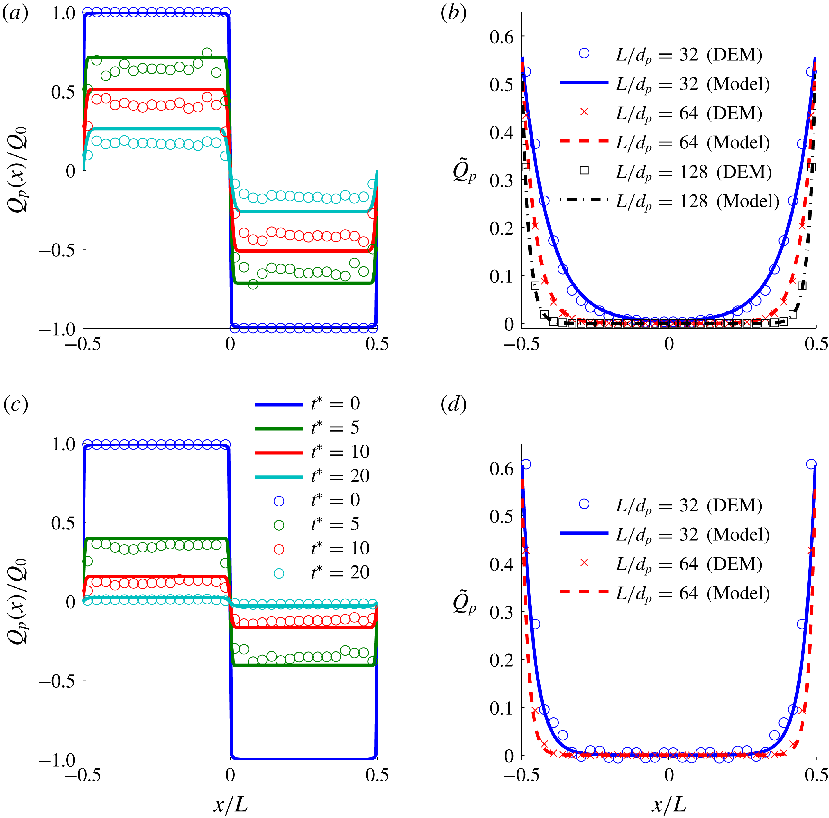
Figure 1 shows both the periodic channel and box simulation results and the model predictions for $0.25$ and $0.35$ volume fractions. As can be seen from the figure, the developed model predictions are close to the particle dynamics simulation results for $\langle \unicode[STIX]{x1D6FC}_{p}\rangle =0.35$ , but differ slightly for moderate volume fraction $\langle \unicode[STIX]{x1D6FC}_{p}\rangle =0.25$ . We noted the results become exact if the triboelectric conductivity $\unicode[STIX]{x1D70E}_{q}$ was increased by ${\sim}10\,\%$ and ${\sim}20\,\%$ for the volume fractions $0.35$ and $0.25$ , respectively.

Figure 1.

(a) Periodic box simulation with $\langle \unicode[STIX]{x1D6FC}_{p}\rangle =0.25$ , (b) periodic channel with $\langle \unicode[STIX]{x1D6FC}_{p}\rangle =0.25$ , (c) periodic box simulation with $\langle \unicode[STIX]{x1D6FC}_{p}\rangle =0.35$ and (d) periodic channel with $\langle \unicode[STIX]{x1D6FC}_{p}\rangle =0.35$ . The time for the periodic box is scaled by $t^{\ast }=t\sqrt{\unicode[STIX]{x1D6E9}}/d_{p}$ and the charge in the beginning of the simulation is $Q_{0}=\pm 10^{-15}$ . The equilibrium charge for the channel simulations is $q_{eq}=15.6\,\text{fC}$ . The channel width for the periodic channel simulations was varied and is given in the legend of (b) and (d). The radial distribution functions at contact were estimated from the DEM data and are $1.8$ and $2.5$ for $\langle \unicode[STIX]{x1D6FC}_{p}\rangle =0.25$ and $\langle \unicode[STIX]{x1D6FC}_{p}\rangle =0.35$ , respectively.

Figure 2.

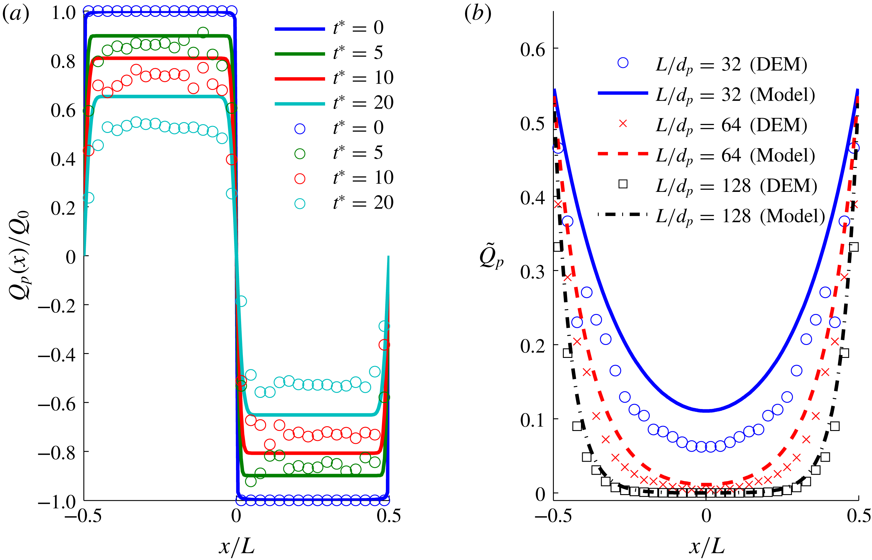
(a) Periodic box simulation with $\langle \unicode[STIX]{x1D6FC}_{p}\rangle =0.15$ and (b) periodic channel with $\langle \unicode[STIX]{x1D6FC}_{p}\rangle =0.15$ . See figure 1 caption for details. The radial distribution function at contact is estimated from the DEM data and is $1.6$ for $\langle \unicode[STIX]{x1D6FC}_{p}\rangle =0.15$ .

Figure 2 shows the periodic box and periodic channel simulation results for a lower volume fraction ( $\langle \unicode[STIX]{x1D6FC}_{p}\rangle =0.15$ ) along with the predictions of the Eulerian model. The model predictions diverge further from DEM simulations results. It was found that the source of difference in the results originated from underpredicting the triboelectric conductivity for this volume fraction by ${\sim}40\,\%$ .

In the periodic domain simulations, the charge density profile remains mostly flat in each half-domain, but decreases in magnitude with increasing time, with transition occurring in a relatively short distance at the boundaries of the half-domains. This pattern can readily be attributed to the dominance of the triboelectric charge conductivity term (which appears through the first term on the right-hand side of (3.2)) in this validation example. This test problem provides a satisfactory validation of the model for triboelectric charge conductivity.

In the wall-bounded tribocharging example, we found that both $\unicode[STIX]{x1D705}_{q}$ and $\unicode[STIX]{x1D705}_{q}^{\ast }$ should be taken into account to capture the spatial variation of charge density. At high particle volume fractions, triboelectric charge diffusivity $\unicode[STIX]{x1D705}_{q}$ is more important than charge diffusion due to particle migration $\unicode[STIX]{x1D705}_{q}^{\ast }$ , since $\unicode[STIX]{x1D705}_{q}/\unicode[STIX]{x1D705}_{q}^{\ast }\propto (\unicode[STIX]{x1D6FC}_{p}g_{0})^{2}$ . At lower particle volume fractions, $\unicode[STIX]{x1D705}_{q}^{\ast }$ contributes more than $\unicode[STIX]{x1D705}_{q}$ . This test problem validates the wall boundary condition and the charge diffusivity models. Taken together, these two examples lend support to all the constitutive models proposed in this study.

Whereas the results from this study cannot be compared with any experiments directly, the higher charge observed at the wall is consistent with the findings of Sowinski et al. (Reference Sowinski, Mayne and Mehrani2012). In the proposed model, the charge distribution in the channel depends on the ratio of triboelectric diffusivity and triboelectric conductivity ( $(\unicode[STIX]{x1D705}_{q}+\unicode[STIX]{x1D705}_{q}^{\ast })/\unicode[STIX]{x1D70E}_{q}$ ). The gradient of charge at the wall becomes steeper as the ratio of diffusivity to conductivity decreases. In particular, when Young’s modulus is decreased both $\unicode[STIX]{x1D705}_{q}$ and $\unicode[STIX]{x1D70E}_{q}$ decrease at the same rate, but $\unicode[STIX]{x1D705}_{q}^{\ast }$ remains unchanged. Hence, for very stiff particles the charge profile would approach a flat line; variation would be confined to a thin boundary layer near the bounding wall and be uniform in the bulk.