1 Introduction
Stirred tank reactors have received considerable attention over the last decades, arising from their many applications in the process and pharmaceutical industries. After initiation of the stirring, fluid is discharged from the impeller, subsequently reaching the tank walls and finally recirculating back to the impeller region. The discharged fluid carries angular momentum which, if not adequately destroyed (e.g. with the use of wall baffles), generates circulation of the fluid bulk in the direction of the impeller rotation. On the rear side of the impeller blades three-dimensional roll vortices are formed, connected with high values of turbulence kinetic energy and shear rate.
One of the most extensively studied features of stirred tanks is their power consumption, as it is directly linked with process efficiency. Numerous investigators (for a review see Maynes & Butcher (Reference Maynes and Butcher2002)) have studied the dependence of power consumption on aspects such as impeller and vessel shape and size at a variety of regimes, ranging from laminar to fully turbulent. This has led to the development of correlation formulae (see for instance Nagata (Reference Nagata1975), Furukawa et al. (Reference Furukawa, Kato, Inoue, Kato, Tada and Hashimoto2012)), enabling accurate power consumption predictions for most of the commonly used configurations.
The bulk of the above studies focus on the steady-state regime, since this is where in practice stirred tanks operate. There are situations, however, where transient power consumption is of interest, as for instance after impulsive increases of the shaft speed, e.g. when initiating the impeller rotation, or when adjusting the shaft speed. In that case spikes in the power/torque of the shaft appear (Maynes & Butcher Reference Maynes and Butcher2002; Steiros et al. Reference Steiros, Bruce, Buxton and Vassilicos2017b ), which may considerably wear the mechanical components of the mixer. Second, prediction of transient power consumption can be useful in the design of systems where the shaft operates at a time-varying speed, for instance following square or sinusoidal waves. Such cases have been shown to promote turbulence intensities and mixing compared to the conventional steady-state operation (Gao et al. Reference Gao, Acharya, Wang and Uhm2004; Roy & Acharya Reference Roy and Acharya2011; Woziwodzki Reference Woziwodzki2011), and can therefore be of interest to a variety of applications.
Literature concerning transient power consumption in stirred tanks is limited: Nagata (Reference Nagata1975) postulated that immediately after the start of impeller operation in a quiescent fluid, the normalised power will reach the maximum possible value, and conducted experiments to measure it. Maynes, Klewicki & Mcmurtry (Reference Maynes, Klewicki and Mcmurtry1999) and Maynes & Butcher (Reference Maynes and Butcher2002) performed a more in-depth analysis of the time evolution of the power consumption after an impulsive increase of shaft speed from zero, by conducting power measurements of various rotating bluff bodies in stirred tanks of different sizes. Three stages were identified in the full transition period: first, a ‘build-up’ regime, where the normalised power remains relatively constant, and the flow field in the vicinity of the bluff body was supposed similar to the one corresponding to rotation in an infinite medium. Second, a ‘decay’ regime, starting the moment when the discharged fluid from the bluff body recirculates back for the first time. During this regime the normalised power drops, until it finally reaches the steady-state regime, where the angular momentum production by the bluff body is equal to the angular-momentum destruction by the tank walls. From these data, correlation formulae were developed, predicting the power values and time scales corresponding to the different transition stages, for various sizes of bluff bodies and tanks. Yoshida et al. (Reference Yoshida, Ito, Yamagiwa, Ohkawa, Abe, Tezura and Shimazaki2001) and Woziwodzki (Reference Woziwodzki2011) conducted torque measurements in cases where the impeller rotated by a small angle in a forward–reverse manner, with the angular velocity following sinusoidal and triangle waves respectively. The instantaneous torque was assumed to be given by a linear sum of a drag and an inertial term, which scaled with the square of the shaft angular velocity and the shaft acceleration, respectively. The relative contribution of the two terms was then tuned using data fitting.
In the above works, the proposed predictions are limited to correlations, restricted to the special case studied and not taking into account the underlying physics of the problem. In this article, we develop a theoretical framework, based on angular momentum balance, under which we derive analytical relations for the prediction of the power consumption of stirred tanks whose shaft speed undergoes impulsive or smooth changes. The predictions are subsequently experimentally validated.
The structure of the article is as follows: in § 2 a theoretical framework is developed which is used to create a model for the prediction of the impeller torque/power number, immediately after an impulsive change in shaft speed. The model is subsequently experimentally validated. In § 3, the above model is used to derive an ordinary differential equation which describes the transient power number of stirred tanks, in quasi-stationary conditions. Predictions of this equation are then experimentally validated. In § 4 the implications of the above analysis on the steady-state power number of unbaffled tanks in turbulent conditions and the applicability of the models are discussed. Finally, § 5 draws the conclusions of this study.
2 Power number immediately after an impulsive change of shaft speed
This section introduces a model based on angular-momentum balance for the prediction of the power number immediately after an impulsive change in shaft speed, starting from a previous steady state. The results are subsequently experimentally validated.
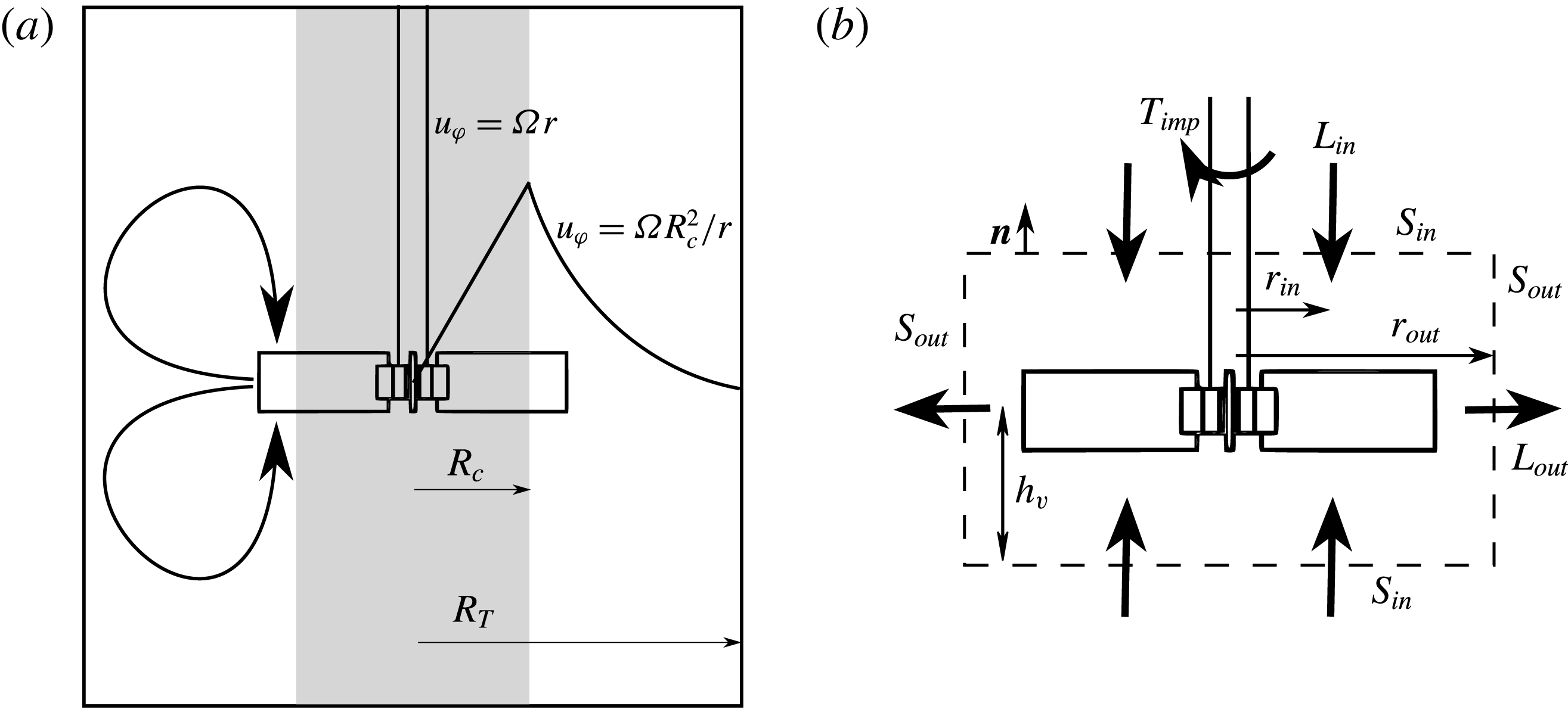
(a) Combined Rankine vortex model in a stirred tank. The grey zone denotes the ‘forced vortex’, while the white zone the ‘free vortex’. (b) Cylindrical control volume around the impeller where the angular-momentum budget is performed for the formulation of Euler’s equation. The total control volume boundary is
 $S=S_{in}+S_{out}$
.

2.1 ‘Extent’ of the solid-body rotation in the tank
Combining the tangential momentum equation with the continuity equation, and multiplying the resulting equation by
 $r$
we obtain the angular-momentum transport equation in the tank in conservative form, i.e.
 $$\begin{eqnarray}\frac{\unicode[STIX]{x2202}r\unicode[STIX]{x1D70C}u_{\unicode[STIX]{x1D719}}}{\unicode[STIX]{x2202}t}\!+\frac{1}{r}\frac{\unicode[STIX]{x2202}r^{2}\unicode[STIX]{x1D70C}u_{\unicode[STIX]{x1D719}}u_{r}}{\unicode[STIX]{x2202}r}\!+\frac{\unicode[STIX]{x2202}\unicode[STIX]{x1D70C}u_{\unicode[STIX]{x1D719}}^{2}}{\unicode[STIX]{x2202}\unicode[STIX]{x1D719}}+\frac{\unicode[STIX]{x2202}r\unicode[STIX]{x1D70C}u_{\unicode[STIX]{x1D719}}u_{z}}{\unicode[STIX]{x2202}z}=\frac{1}{r}\frac{\unicode[STIX]{x2202}}{\unicode[STIX]{x2202}r}(r^{2}\unicode[STIX]{x1D70F}_{r\unicode[STIX]{x1D719}})\!+\frac{1}{r}\frac{\unicode[STIX]{x2202}}{\unicode[STIX]{x2202}\unicode[STIX]{x1D719}}(-rp+r\unicode[STIX]{x1D70F}_{\unicode[STIX]{x1D719}\unicode[STIX]{x1D719}})\!+\frac{\unicode[STIX]{x2202}}{\unicode[STIX]{x2202}z}(r\unicode[STIX]{x1D70F}_{\unicode[STIX]{x1D719}z}),\end{eqnarray}$$
where
 $u_{i}$
is the fluid velocity in cylindrical coordinates,
 $\unicode[STIX]{x1D70F}_{ij}$
is the stress tensor (
 $i$
and
 $j$
can be
 $r$
,
 $\unicode[STIX]{x1D719}$
or
 $z$
),
 $\unicode[STIX]{x1D70C}$
is the fluid density and
 $p$
is the pressure field. Note that in the above equation we have assumed an axisymmetric gravitational potential. We consider a stationary and ergodic process, we time average (2.1) and integrate it in a cylindrical volume around the impeller (see figure 1), i.e.
 $$\begin{eqnarray}\int _{0}^{t_{m}}\int _{-h_{v}}^{h_{v}}\int _{0}^{r_{out}}\int _{0}^{2\unicode[STIX]{x03C0}}(\cdot )\frac{r}{t_{m}}\,\text{d}\unicode[STIX]{x1D719}\,\text{d}r\,\text{d}z\,\text{d}t,\end{eqnarray}$$
where
 $t_{m}$
is a time when the terms of (2.1) are statistically converged and
 $r_{out}$
and
 $h_{v}$
are the radius and mid-height respectively, of the cylindrical control volume. Note that in that case time averaging is identical to ensemble averaging
 $\langle \cdot \rangle$
(i.e. averaging over many realisations). After the integration we obtain
 $$\begin{eqnarray}T_{imp}=\left\langle \int _{S}\unicode[STIX]{x1D70C}ru_{\unicode[STIX]{x1D719}}u_{n}\,\text{d}S-\int _{S_{in}}r\unicode[STIX]{x1D70F}_{z\unicode[STIX]{x1D719}}n_{i}e_{i}\,\text{d}S-\int _{S_{out}}r\unicode[STIX]{x1D70F}_{r\unicode[STIX]{x1D719}}\,\text{d}S\right\rangle ,\end{eqnarray}$$
where
 $T_{imp}$
is the ensemble-averaged impeller torque,
 $u_{n}=u_{i}n_{i}$
,
 $n_{i}$
being the
 $i$
th component of the unity vector normal to the boundary area of the cylindrical volume,
 $S$
, and
 $e_{i}$
is the
 $i$
th component of the axial unit vector.
 $S_{in}$
and
 $S_{out}$
are the boundary areas corresponding to the impeller inlet (
 $\langle u_{n}\rangle <0$
, cylinder bases) and outlet (
 $\langle u_{n}\rangle >0$
, cylinder side) respectively, with
 $S=S_{in}+S_{out}$
(see figure 1). Note that in the integration we made use of the periodicity in
 $\unicode[STIX]{x1D719}$
. Assuming that the contribution of the viscous terms is negligible (a realistic assumption in turbulent tanks as shown in Başbuğ, Papadakis & Vassilicos (Reference Başbuğ, Papadakis and Vassilicos2017)), equation (2.3) can be written in the form
 $$\begin{eqnarray}T_{imp}={\dot{m}}(L_{out}-L_{in}),\end{eqnarray}$$
which is Euler’s turbine equation. In the above equation
 ${\dot{m}}=\langle \int _{S_{out}}\unicode[STIX]{x1D70C}u_{n}\,\text{d}S\rangle =-\langle \int _{S_{in}}\unicode[STIX]{x1D70C}u_{n}\,\text{d}S\rangle$
is the ensemble-averaged mass flow rate of the impeller. The quantity
 $L_{k}$
, where
 $k$
can be either in or out, is the ensemble-averaged angular momentum entering or exiting the impeller region normalised by the mass flow rate, and is given by
 $$\begin{eqnarray}L_{k}=\frac{\left\langle \displaystyle \int _{S_{k}}\unicode[STIX]{x1D70C}ru_{\unicode[STIX]{x1D719}}u_{n}\,\text{d}S\right\rangle }{\left\langle \displaystyle \int _{S_{k}}\unicode[STIX]{x1D70C}u_{n}\,\text{d}S\right\rangle }.\end{eqnarray}$$
The quantity
 $L_{in}$
or its non-dimensional form
 $l_{in}=L_{in}/\unicode[STIX]{x1D6FA}R^{2}$
, where
 $\unicode[STIX]{x1D6FA}=2\unicode[STIX]{x03C0}N$
is the angular velocity of the shaft and
 $R=D/2$
is the impeller radius, can be used to quantify the ‘extent’ of the steady-state solid-body rotation in the tank: in the special case in which there is no solid-body rotation it can readily be shown that
 $l_{in}=0$
. As the solid-body rotation grows,
 $l_{in}$
grows as well and as the fluid’s tangential velocity approaches that of the impeller we have
 $L_{in}\rightarrow L_{out}$
, while
 $L_{out}\rightarrow \unicode[STIX]{x1D6FA}R^{2}$
. Therefore in that case
 $l_{in}\rightarrow 1$
. Note that
 $l_{in}$
cannot describe the solid-body rotation with the same angular velocity as the impeller’s, since in that case the mass flow rate vanishes and
 $l_{in}$
is not defined, i.e.
 $l_{in}\neq 1$
.
The above can be understood better using the fact that the ensemble-averaged solid-body rotation in the tank can be modelled as a Rankine vortex (see figure 1), as shown by Nagata (Reference Nagata1975). This is a cylindrically rotating zone where the fluid rotates with the same angular velocity as the impeller (forced vortex) for
 $r<R_{c}<R$
, where
 $R_{c}$
is the forced vortex radius, followed by a region where the angular momentum is assumed constant (free vortex) at larger radii.
For the free vortex model to hold, two conditions must be met, i.e. a prevalent tangential motion in the tank (in fact the secondary recirculatory flows are neglected) and negligible viscous effects; in other words small local Ekman (the ratio of viscous acceleration to Coriolis force) and Rossby (the ratio of nonlinear inertial acceleration to Coriolis force) numbers. In that case the flow also satisfies the Taylor–Proudman constraint of columnar motion (i.e. no axial velocity variation) and thus, the tangential velocity is expected to be a function of the radial distance only. Nagata (Reference Nagata1975) suggested that the above conditions can be thought realistic in the bulk of an unbaffled tank operating at a turbulent regime. Indeed, his measurements showed that the tangential velocity distribution approaches a Rankine profile in turbulent unbaffled tanks stirred by radial impellers, while the axial variation of the tangential velocity is small, with the exception of the zones near the vessel top and bottom walls, where the wall friction acts. The above have led to the widespread use of the Rankine vortex, for instance when modelling the free-surface shape of uncovered unbaffled tanks (see for instance Nagata (Reference Nagata1975), Busciglio, Caputo & Scargiali (Reference Busciglio, Caputo and Scargiali2013)). It is important to note that the Rankine vortex profile has been used/validated for ‘standard’ configurations (i.e.
 $D_{T}\approx H$
,
 $0.3<D/D_{T}<0.5$
, where
 $D_{T}$
and
 $H$
are the tank’s diameter and height respectively). It is therefore not certain that the model holds in drastically different geometries (for instance when the tank height is very large).
We may therefore model the ensemble-averaged tangential fluid velocity in an unbaffled turbulent tank as
 $\langle u_{\unicode[STIX]{x1D719}}\rangle =\unicode[STIX]{x1D6FA}r$
for
 $r<R_{c}$
(forced vortex) and
 $\langle u_{\unicode[STIX]{x1D719}}\rangle =\unicode[STIX]{x1D6FA}R_{c}^{2}/r$
for
 $r\geqslant R_{c}$
(free vortex). Decomposing the velocity in its mean and fluctuating parts, i.e.
 $u_{i}=\langle u_{i}\rangle +u_{i}^{\prime }$
, we may further assume that in the impeller inlet (
 $S_{in}$
in figure 1) the contribution of the cross-term
 $\langle u_{n}^{\prime }u_{\unicode[STIX]{x1D719}}^{\prime }\rangle$
is very small when calculating
 $l_{in}$
, and neglect it. As shown in Başbuğ et al. (Reference Başbuğ, Papadakis and Vassilicos2017), this assumption is realistic for transitional and turbulent unbaffled tanks stirred by radial turbines (i.e.
 $l_{in}$
changes by less than 1 % if
 $\langle u_{n}^{\prime }u_{\unicode[STIX]{x1D719}}^{\prime }\rangle$
is neglected). From the above, equation (2.5) reduces to
 $$\begin{eqnarray}l_{in}=\frac{2\unicode[STIX]{x1D6FA}R_{c}^{2}\displaystyle \int _{0}^{2\unicode[STIX]{x03C0}}\int _{R_{c}}^{r_{out}}\unicode[STIX]{x1D70C}\langle u_{n}\rangle r\,\text{d}r\,\text{d}\unicode[STIX]{x1D719}}{2\unicode[STIX]{x1D6FA}R^{2}\displaystyle \int _{0}^{2\unicode[STIX]{x03C0}}\int _{R_{c}}^{r_{out}}\unicode[STIX]{x1D70C}\langle u_{n}\rangle r\,\text{d}r\,\text{d}\unicode[STIX]{x1D719}}=\left(\frac{R_{c}}{R}\right)^{2},\end{eqnarray}$$
where the lower limit of integration for the radial coordinate is not zero since the blade does not pump fluid for
 $r<R_{c}$
(forced vortex), while the factor
 $2$
in the numerator and denominator is due to the two bases of the control volume. From (2.6) it is clear that
 $l_{in}$
becomes zero when there is no solid-body rotation in the tank (
 $R_{c}=0$
), while
 $l_{in}$
tends to
 $1$
when the fluid approaches the angular velocity of the impeller (for
 $R_{c}=R$
the mass flow rate vanishes and (2.6) is not valid).
2.2 Power number dependence on solid-body rotation
Using (2.4), we may develop a low-order model linking the impeller power number with
 $l_{in}$
. For this, we first assume that the quantities
 ${\dot{m}}/{\dot{m}}_{\infty }$
and
 $L_{out}/L_{\infty }$
, where the subscript
 $\infty$
signifies evaluation of the quantities when there is no solid-body rotation in the tank (or in an infinite medium), can be adequately modelled as functions of
 $l_{in}$
, instead of the full velocity and pressure distributions.
Regarding the mass flow rate, we expect that it is a decreasing function of
 $l_{in}$
(keeping the shaft velocity constant). That is, because as
 $l_{in}$
increases, the solid-body rotation increases as well, and thus the relative blade velocity decreases. In the limiting case of
 $l_{in}\rightarrow 1$
we have
 ${\dot{m}}\rightarrow 0$
since the relative velocity of the blades approaches zero. We model this behaviour with a decreasing power law, i.e.
 $$\begin{eqnarray}{\dot{m}}={\dot{m}}_{\infty }(1-l_{in})^{a},\end{eqnarray}$$
where
 $a\geqslant 0$
is an arbitrary exponent. Note that when
 $a=0$
,
 ${\dot{m}}={\dot{m}}_{\infty }$
no matter the operating conditions (ideal impeller behaviour), while when
 $a=1$
we assume a linear drop of the mass flow rate.
For the quantity
 $L_{out}$
we expect that it is an increasing function of
 $l_{in}$
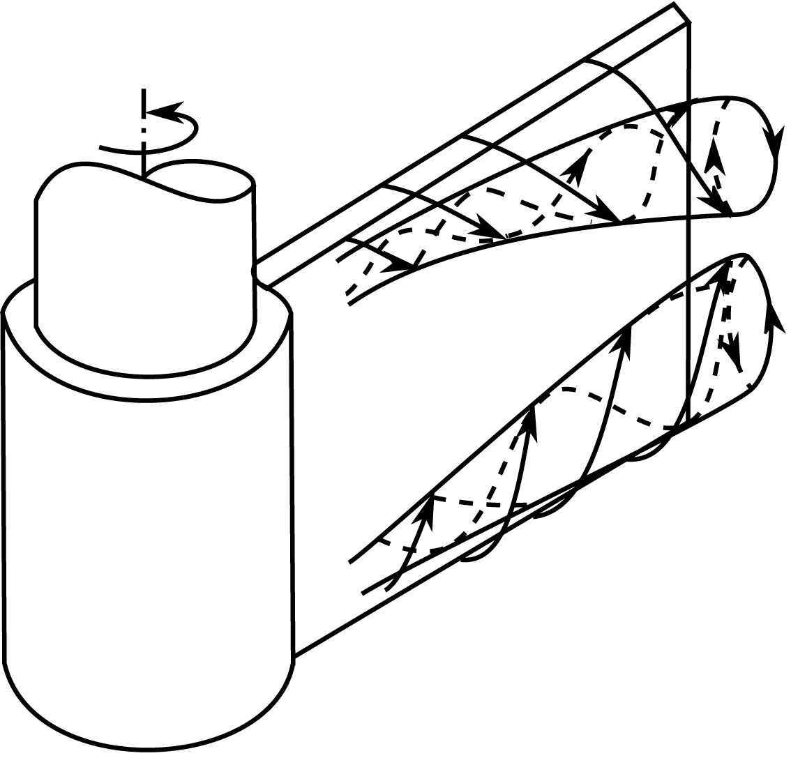
for flat and forward-swept turbines. That is, because as the solid-body rotation expands in the tank, the fluid separation from the impeller occurs at larger radii (see figure 2), causing in turn larger discharged tangential fluid velocities. In the limit of
 $l_{in}\rightarrow 1$
we have
 $L_{out}\rightarrow \unicode[STIX]{x1D6FA}R^{2}$
, as the separation point approaches the blade tip. We model this behaviour as linear, i.e.
 $$\begin{eqnarray}L_{out}=L_{\infty }+(\unicode[STIX]{x1D6FA}R^{2}-L_{\infty })l_{in}.\end{eqnarray}$$
In the above equation if
 $L_{\infty }=\unicode[STIX]{x1D6FA}R^{2}$
, then
 $L_{out}=\unicode[STIX]{x1D6FA}R^{2}$
no matter the input conditions (ideal impeller behaviour). Note that in the above models we have assumed that the fluid rotates in the same sense as the impeller, i.e.
 $l_{in}\geqslant 0$
. Furthermore, we have assumed that the fluid is pumped in a ‘canonical’ way from the blades’ tip back to the impeller hub, as depicted in figure 1. For this to happen, the fluid’s tangential velocity in between the blades has to be smaller than the impeller’s, imposing
 $l_{in}<1$
. Therefore, equations (2.7) and (2.8) can be considered valid for
 $l_{in}\in [0,1)$
.
Schematic diagram of the roll vortices’ separation at the rear side of the blades, after Winardi & Nagase (Reference Winardi and Nagase1994).

Substituting (2.7) and (2.8) to (2.4) we obtain
 $$\begin{eqnarray}T_{imp}={\dot{m}}_{\infty }L_{\infty }(1-l_{in})^{1+a}.\end{eqnarray}$$
If both sides of (2.9) are multiplied with
 $2\unicode[STIX]{x03C0}/\unicode[STIX]{x1D70C}N^{2}D^{5}$
, we obtain the following expression for the power number of the impeller
 $$\begin{eqnarray}Np=Np_{\infty }(1-l_{in})^{1+a},\end{eqnarray}$$
where
 $Np_{\infty }=Np_{\infty }(Re)$
is the power number of the impeller under conditions of zero solid-body rotation in the tank. Note that
 $Re=ND^{2}/\unicode[STIX]{x1D708}$
for stirred tanks, where
 $\unicode[STIX]{x1D708}$
is the kinematic viscosity of the fluid. In (2.10)
 $l_{in}\in [0,1)$
and
 $a>0$
. In the special case of
 $a=0$
(ideal impeller) the impeller performance (e.g. mass flow rate, output swirl) is supposed not to be affected by the solid-body rotation. By repositioning of its terms, equation (2.10) becomes
 $$\begin{eqnarray}T_{imp}=\frac{4}{\unicode[STIX]{x03C0}^{3}}\unicode[STIX]{x1D70C}RNp_{\infty }R^{2}(R\unicode[STIX]{x1D6FA})^{1-a}(R\unicode[STIX]{x1D6FA}-R\unicode[STIX]{x1D6FA}l_{in})^{1+a}.\end{eqnarray}$$
Equation (2.11) may be interpreted as follows:
 $Np_{\infty }=Np_{\infty }(Re)$
is a drag-like coefficient of the impeller, while
 $R\unicode[STIX]{x1D6FA}$
and
 $R\unicode[STIX]{x1D6FA}-R\unicode[STIX]{x1D6FA}l_{in}$
are the two characteristic velocities which affect the impeller torque. Specifically,
 $R\unicode[STIX]{x1D6FA}l_{in}$
can be interpreted as the characteristic velocity of the solid-body rotation, in the sense that
 $l_{in}$
quantifies the extent of the solid-body rotation (as explained in § 2.1) and
 $R\unicode[STIX]{x1D6FA}$
its (limiting) speed. Therefore
 $R\unicode[STIX]{x1D6FA}-R\unicode[STIX]{x1D6FA}l_{in}$
can be thought as the characteristic relative velocity of the blades, a standard scaling quantity for bodies performing linear motion. The other velocity,
 $R\unicode[STIX]{x1D6FA}$
, is that of the impeller tip and its presence in (2.11) arises from the fact that there are forces affecting the flow field which scale with the rotational velocity itself (i.e. centrifugal and Coriolis forces). In the special case of
 $a=1$
we assume that these forces either do not affect the drag of the rotating body or, more generally, that their effects scale with the characteristic relative velocity of the blades. Based on (2.11) we may define the following torque coefficient for a mixing impeller
 $$\begin{eqnarray}C_{m}=\frac{2T_{imp}}{RA\unicode[STIX]{x1D70C}(R\unicode[STIX]{x1D6FA})^{1-a}(R\unicode[STIX]{x1D6FA}-r_{w}\unicode[STIX]{x1D714}_{w})^{1+a}},\end{eqnarray}$$
where
 $r_{w}\unicode[STIX]{x1D714}_{w}$
is the characteristic tangential velocity of the fluid and
 $A$
is the frontal area of the blades. If we assume that
 $r_{w}\unicode[STIX]{x1D714}_{w}$
scales with
 $R\unicode[STIX]{x1D6FA}$
(self-similar regime), equation (2.12) becomes
 $$\begin{eqnarray}C_{m}^{\prime }=\frac{2T_{imp}}{RA\unicode[STIX]{x1D70C}(\unicode[STIX]{x1D6FA}R)^{2}},\end{eqnarray}$$
which is essentially the conventional definition of power number for mixing impellers, i.e. the conventional power number can be considered a function of
 $Re$
exclusively, only if the flow is self-similar with increasing
 $Re$
.
2.3 Power number immediately after an impulsive change of shaft speed
Using the previous analysis we can have an estimate of the impeller torque/power immediately after an impulsive change of the shaft speed. This is based on the assumption that after an impulsive speed change there exists a time interval during which the quantity
 $L_{in}$
is constant and equal to what it was before the speed change. Simply put, if the impeller operates at a steady rotational frequency
 $N_{0}$
(henceforth referred to simply as speed) corresponding to
 $L_{in0}$
and if at
 $t=0$
we instantaneously change the shaft speed to
 $N_{2}$
, then until
 $t=t_{p}$
, we assume that
 $L_{in2}=L_{in0}$
. Note that the subscripts
 $0$
and
 $2$
of a quantity determine at which shaft speed it is evaluated and, in the case of normalised quantities, with which speed it is normalised.
The above assumption is linked with the recirculating pattern in the tank, i.e. the cycle where fluid is discharged from the impeller, reaches the wall and then returns to the impeller region (see figure 1). Therefore, for the duration of one recirculation cycle after a change of shaft speed (
 $0<t<t_{p}$
), the ensemble-averaged tangential velocity profile at the top and bottom boundaries of the impeller control volume remains unchanged (see figure 1), since the discharged fluid after the impulsive change has not reached there yet. This means that
 $\langle u_{\unicode[STIX]{x1D719}}(r)\rangle$
in (2.5) is the same as before the speed change. Assuming a Rankine vortex, the angular-momentum profiles at the top and bottom boundaries of the control volume are
 $\langle ru_{\unicode[STIX]{x1D719}}\rangle =\unicode[STIX]{x1D6FA}_{0}r^{2}$
for
 $r<R_{c}$
and
 $\langle ru_{\unicode[STIX]{x1D719}}\rangle =\unicode[STIX]{x1D6FA}_{0}R_{c}^{2}$
for
 $r\geqslant R_{c}$
, before as well as immediately after the change in shaft speed. Before the speed change, fluid is not pumped for
 $r<R_{c}$
, since the relative velocity there is zero. Therefore, we can deduce from (2.5) (assuming that the contribution of the cross-term
 $\langle u_{n}^{\prime }u_{\unicode[STIX]{x1D719}}^{\prime }\rangle$
is negligible when calculating
 $L_{in}$
, see § 2.1) that
 $L_{in0}=\unicode[STIX]{x1D6FA}_{0}R_{c}^{2}$
. However, immediately after the speed increase the relative blade velocity is greater than zero for
 $r<R_{c}$
, and some fluid is subsequently pumped, leading to
 $L_{in2}<L_{in0}$
from (2.5). Therefore, the assumption that
 $L_{in2}\approx L_{in0}$
implies that the fluid which is pumped in the forced vortex region (
 $r<R_{c}$
), after the speed change, is negligible. This could be realistic in turbulent conditions, given that then, the mass flow rate scales with
 $D^{3}$
(Nagata Reference Nagata1975), and therefore smaller radii pump significantly less fluid.
From the above, in the special case of
 $N_{0}=0$
,
 $L_{in2}=L_{in0}=0$
and using (2.10) we obtain
 $$\begin{eqnarray}Np_{2}=Np_{\infty 2},\end{eqnarray}$$
where
 $Np_{2}$
corresponds to the power number after the impulsive speed increase and before the solid-body rotation in the tank changes (
 $0<t<t_{p}$
). If
 $N_{0}>0$
then
 $Np_{\infty 0}$
,
 $l_{in0}$
and
 $Np_{s0}$
are defined (
 $Np_{s}$
being the steady-state power number), while
 $l_{in2}=l_{in0}N_{0}/N_{2}$
given that we assumed
 $L_{in2}=L_{in0}$
. Using (2.10) we obtain
 $$\begin{eqnarray}\displaystyle Np_{s0} & = & \displaystyle Np_{\infty 0}(1-l_{in0})^{1+a}\end{eqnarray}$$
 $$\begin{eqnarray}\displaystyle Np_{2} & = & \displaystyle Np_{\infty 2}\left(1-l_{in0}\frac{N_{0}}{N_{2}}\right)^{1+a}.\end{eqnarray}$$
 $l_{in0}$
from (2.15a
) to (2.15b
) we obtain
 $$\begin{eqnarray}\frac{Np_{\infty 0}^{1/(1+a)}-Np_{2}^{1/(1+a)}R_{\infty 0}^{1/(1+a)}}{Np_{\infty 0}^{1/(1+a)}-Np_{s0}^{1/(1+a)}}=\frac{N_{0}}{N_{2}},\end{eqnarray}$$
where
 $R_{\infty 0}=Np_{\infty 0}/Np_{\infty 2}$
. Equation (2.16) gives an estimate of the power number immediately after the impulsive change in shaft speed,
 $Np_{2}$
, for a given
 $a>0$
. Note that (2.16) is valid for
 $N_{2}>N_{w}$
, where
 $N_{w}$
is the mean rotational frequency of the fluid in between the blades (
 $N_{w}<N_{0}$
). This is because (2.10) is not valid if the fluid has the same or larger angular velocity compared to the impeller, as explained in § 2.2. In the limiting case of
 $N_{2}=N_{w}$
we expect
 $Np_{2}=0$
and therefore (2.16) becomes
 $$\begin{eqnarray}N_{w}=N_{0}\left[1-\left(\frac{Np_{s0}}{Np_{\infty 0}}\right)^{1/(1+a)}\right].\end{eqnarray}$$
The above equation gives an estimate of the mean tangential velocity of the fluid in between the blades during steady conditions.
If during a steady state (with
 $N_{0}>0$
) the impeller immediately stops, i.e.
 $N_{2}=0$
, then for a limited time interval the impeller blades behave approximately like stationary bluff bodies in a shear flow with a mean velocity gradient of
 $2\unicode[STIX]{x03C0}N_{w}$
and a median velocity of
 $\unicode[STIX]{x03C0}N_{w}R$
. In that case we expect that the torque scales with
 $N_{w}^{2}$
, much like a wall baffle. Using (2.17) we obtain
 $$\begin{eqnarray}Np_{stop}\propto \left[1-\left(\frac{Np_{s0}}{Np_{\infty 0}}\right)^{1/(1+a)}\right]^{2},\end{eqnarray}$$
where in
 $Np_{stop}$
the normalisation speed is
 $N_{0}$
. The above predictions can be summarised as follows
 $$\begin{eqnarray}\left\{\begin{array}{@{}ll@{}}\displaystyle Np_{2}=Np_{\infty 2},\quad & N_{0}=0\\ \displaystyle \frac{Np_{\infty 0}^{1/(1+a)}-Np_{2}^{1/(1+a)}R_{\infty 0}^{1/(1+a)}}{Np_{\infty 0}^{1/(1+a)}-Np_{s0}^{1/(1+a)}}=\frac{N_{0}}{N_{2}},\quad & N_{0}>0,N_{2}>N_{w}\\ \displaystyle Np_{stop}\propto \left[1-\left(\frac{Np_{s0}}{Np_{\infty 0}}\right)^{1/(1+a)}\right]^{2},\quad & N_{2}=0.\end{array}\right.\end{eqnarray}$$
Listed below are the necessary assumptions for (2.19) to be valid.
-
(i) The torque due to shear stresses on the boundaries of the control volume of figure 1 is negligible.
-
(ii) The quantities
 ${\dot{m}}/{\dot{m}}_{\infty }$
and
$L_{out}/L_{\infty }$
are functions of
$l_{in}$
, as shown in (2.7) and (2.8).
-
(iii) For an impulsive change of shaft speed from
$N_{0}$
to
$N_{2}$
there is a time interval, starting the moment of speed change, where
$L_{in2}=L_{in0}$
.


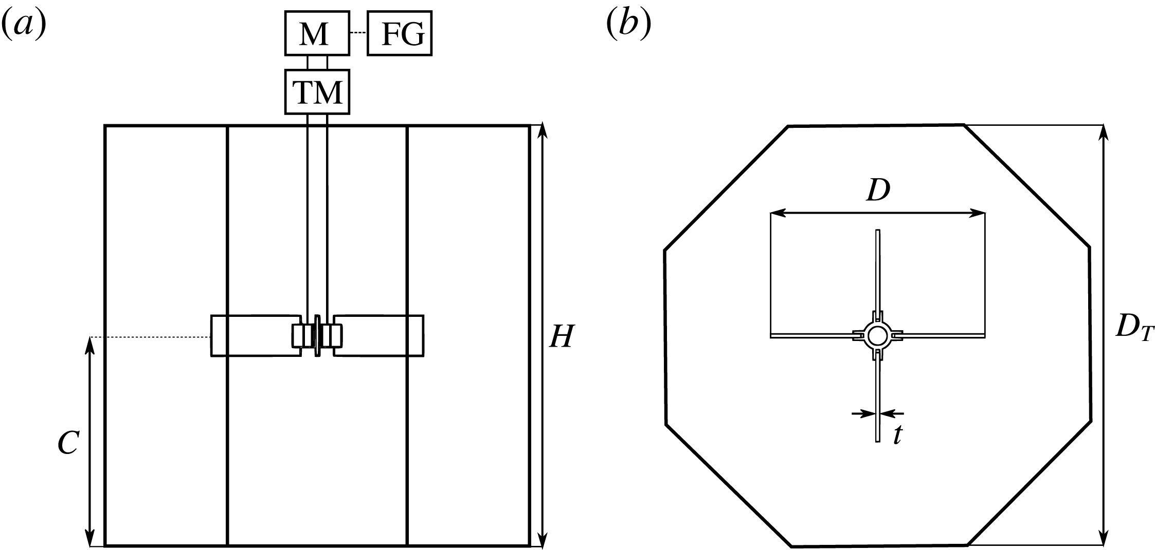
Side and top views of the stirred tank used in the experiments:
 $D_{T}=H=45~\text{cm}$
;
 $C=H/2$
;
 $D\approx D_{T}/2$
;
 $t=4~\text{mm}$
. TM: torque meter, M: motor, FG: function generator.

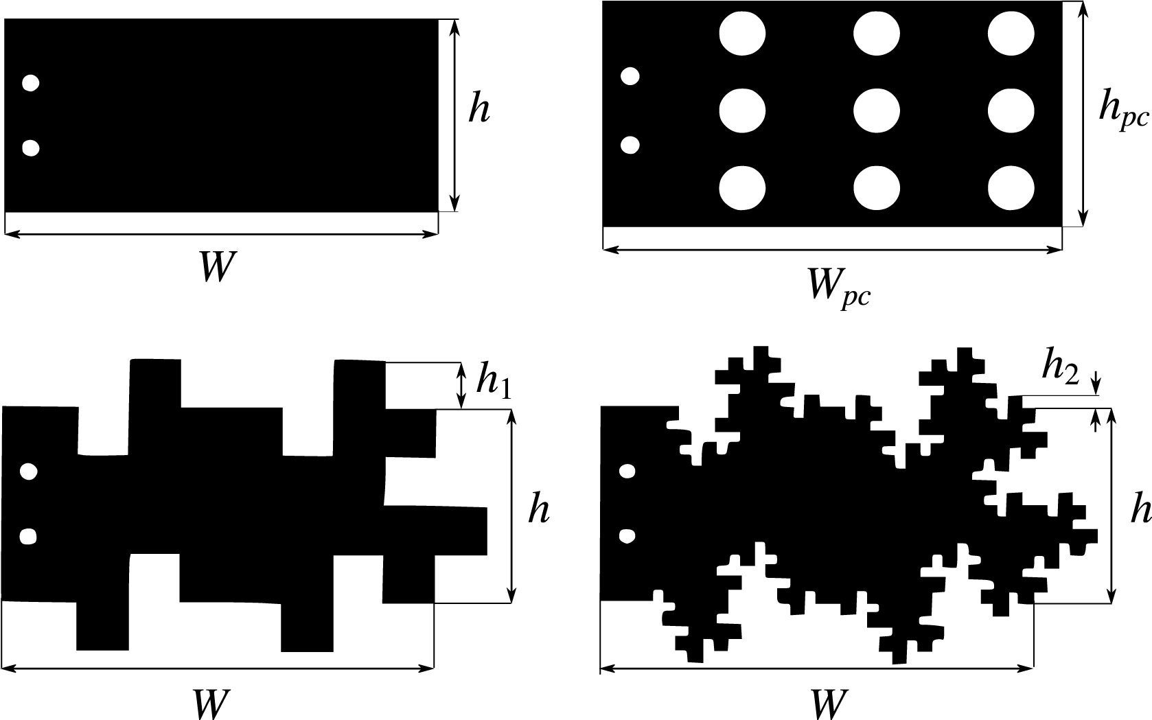
Regular (R), perforated (PC), fractal1 (F1) and fractal2 (F2) blades used in the experiments:
 $W=95~\text{mm}$
;
 $h=4h_{1}=16h_{2}=44.8~\text{mm}$
;
 $W_{pc}=98.5~\text{mm}$
;
 $h_{pc}=50.4~\text{mm}$
. All blades had the same area,
 $A=4228~\text{mm}^{2}$
, and thickness,
 $t_{b}=4~\text{mm}$
.

2.4 Experimental validation
2.4.1 Experimental apparatus
The validation experiments were conducted in an unbaffled, acrylic tank, which was octagonal in shape (see figure 3). The inner diameter of the tank was
 $D_{T}=2R_{T}$
 $=45$
cm, while its height was equal to its diameter, i.e.
 $H=D_{T}$
. The tank was filled with water and a lid was used to prevent free-surface displacement. The impeller used was a four-bladed, flat-blade turbine, mounted in the tank at mid-height. Four versions of the impeller were used by switching different sets of blades on the impeller hub (figure 4). These comprised of regular-rectangular blades (R) commonly used in industry, fractal blades with one and two iterations (F1, F2) whose details are shown in Steiros et al. (Reference Steiros, Bruce, Buxton and Vassilicos2017b
), and perforated blades (PC). As shown in Steiros et al. (Reference Steiros, Bruce, Buxton and Vassilicos2017a
) these blade types generate considerably different flow properties (mass flow rates, turbulence intensities, tip vortices) and could thus help us investigate the generality of the model. All blade types had the same frontal area,
 $A=4228~\text{mm}^{2}$
and same thickness
 $t_{b}=4~\text{mm}$
. The regular impeller had a diameter of
 $D_{R}=223~\text{mm}$
, while for the perforated-blade impeller
 $D_{PC}=230~\text{mm}$
. Regarding the two fractal impellers, their diameters are dependent on the axial position, and for this reason their mean diameters (which were equal to the diameters of the regular impeller) were used as a reference.
The impellers were driven by a stepper motor (Motion Control Products), in microstepping mode (25 000 steps per rotation), to ensure smooth movement. The motor was controlled by a function generator (33 600A, Agilent). The torque of the impellers was measured with an in-line torque transducer (TM306, Magtrol). For the acquisition of the torque signal the default acquisition system was used (DSP 6001, Magtrol), which allowed a maximum acquisition rate of 25 Hz. When higher acquisition rate was necessary, a National Instruments data acquisition system was used (USB-6211, NI), and the acquisition frequency was set to 1 kHz. Throughout the text it will be made clear under which of the two acquisition frequencies the signal was acquired. The rotational speed was monitored with an optical encoder (60 ppr) embedded in the torque transducer. Torque due to friction was monitored when the tank was empty and no blades were attached to the shaft, and was then removed from the actual measurements. Both friction and hydrodynamic torque measurements were found to be reproducible.
2.4.2 Validation experiments
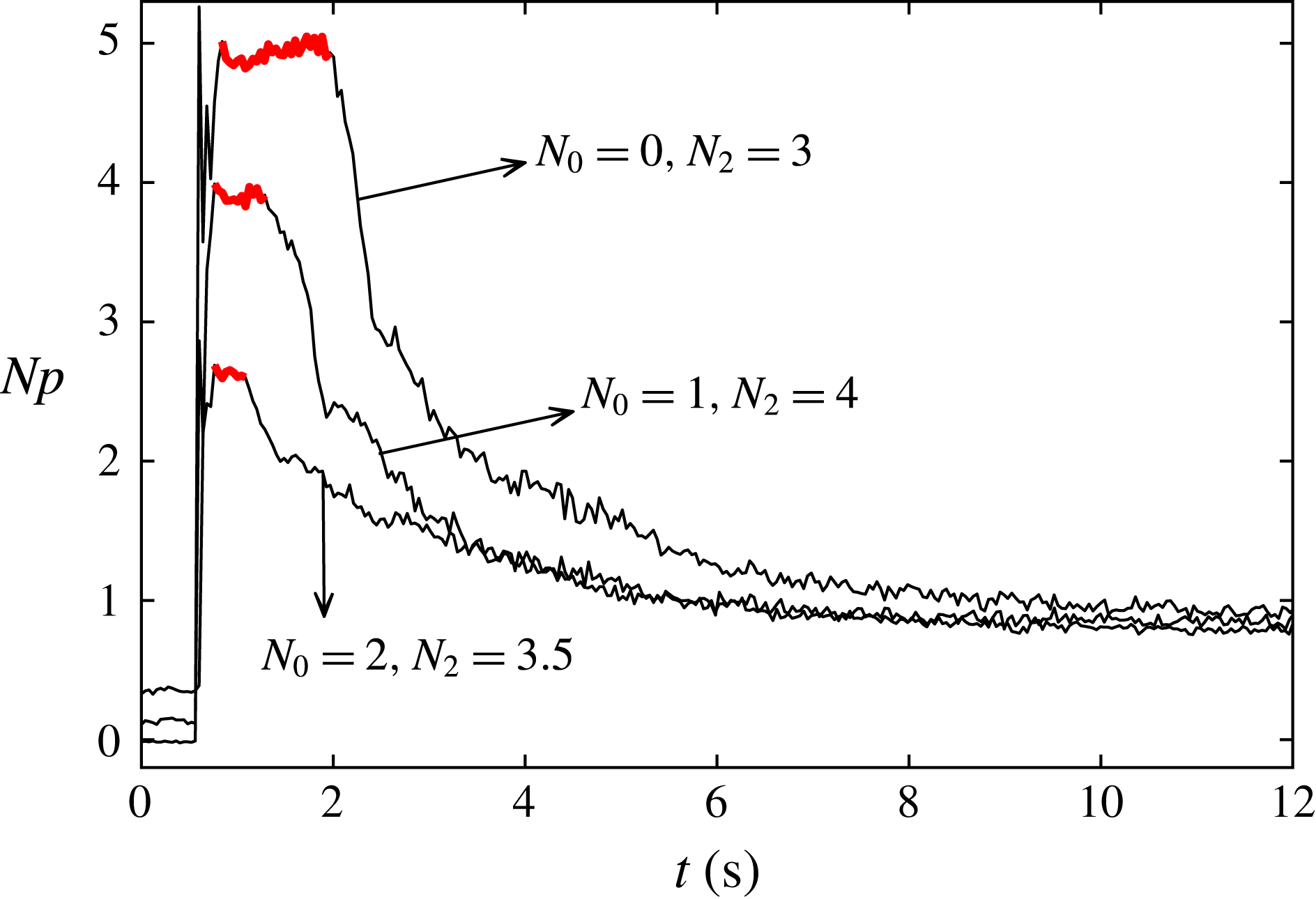
To validate (2.16) torque measurements were performed for the four impeller types shown in figure 4. The acquisition frequency was set to 25 Hz. First, the steady-state,
 $Np_{s}$
, and infinite medium,
 $Np_{\infty }$
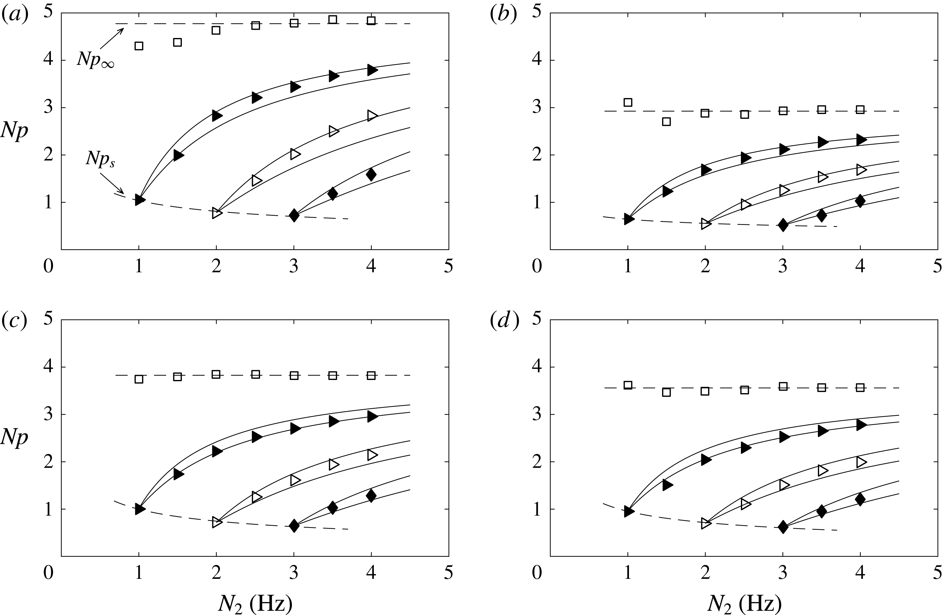
, power numbers were experimentally determined for the four impellers, and are plotted in figure 6. For
 $Np_{\infty }$
, as also shown in Steiros et al. (Reference Steiros, Bruce, Buxton and Vassilicos2017b
), this was done by performing impulsive steps from zero shaft speed to different end speeds, and then monitoring the plateau which appears in the power number time series immediately after the acceleration. This plateau value is
 $Np_{\infty }$
, as shown in (2.14). An example of the power number response after such steps can be seen in figure 5 (case of
 $N_{0}=0$
). The measured
 $Np_{s}$
and
 $Np_{\infty }$
for the different impellers are shown as dashed lines in figure 6. We observe that for all blades the steady-state power number has a declining trend, which is typical for turbulent conditions in unbaffled tanks (see for instance Laity & Treybal (Reference Laity and Treybal1957), Nagata (Reference Nagata1975), Steiros et al. (Reference Steiros, Bruce, Buxton and Vassilicos2017b
)). Indeed, impeller speed of
 $1\leqslant N\leqslant 4$
Hz corresponds to
 $50\,000\leqslant Re\leqslant 200\,000$
which is sufficient for a fully turbulent regime. The infinite medium power number remains relatively constant for all the tested impellers, at least for the highest speeds, as expected in the fully turbulent regime (see Steiros et al. (Reference Steiros, Bruce, Buxton and Vassilicos2017b
)).
Measured power number response after three different types of impulsive steps in the shaft speed (
 $N_{0}$
is the starting speed and
 $N_{2}$
the end speed) for the regular impeller. The red part of the signal signifies the plateau location.

Plateau power number of different end speeds,
 $N_{2}$
, for different starting shaft speeds
 $N_{0}$
. Symbols: measurements. (▫)
 $N_{0}=0$
Hz. (▸)
 $N_{0}=1$
Hz. (▹)
 $N_{0}=2$
Hz. (♦)
 $N_{0}=3$
Hz. Dashed lines: fits from the data for
 $Np_{\infty }$
(top dashed line) and
 $Np_{s}$
(bottom dashed line). Solid lines: predictions using (2.16) for
 $a=0$
(upper line) and
 $a=1$
(bottom line). (a) R impeller, (b) PC impeller, (c) F1 impeller, (d) F2 impeller.

Knowing the values of
 $Np_{s}$
and
 $Np_{\infty }$
, we may use (2.16) to obtain a prediction for the plateau power number after an arbitrary step change in shaft speed, from
 $N_{0}$
to
 $N_{2}$
Hz. In figure 6 these predictions are also plotted (solid lines) corresponding to different step changes. For each case, two solid lines are plotted: one for
 $a=0$
and one for
 $a=1$
. These values of
 $a$
were chosen because they have a physical significance: imposing
 $a=0$
we assume that the impeller performance (e.g. the mass flow rate) is not affected by the solid-body rotation (see § 2.2), and an overestimation of the power number is thus expected. Choice of
 $a=1$
suggests that all blade forces are proportional to the characteristic relative velocity of the blades (see § 2.2). To validate these predictions, the impeller was rotated at a steady speed of
 $N_{0}\in \{1,2,3\}~\text{Hz}$
, and at a given time it was instantly accelerated to
 $N_{2}\in \{1.5,2,2.5,3,3.5,4\}~\text{Hz}$
insofar as
 $N_{2}>N_{0}$
. The power number signal immediately after the acceleration demonstrated a plateau (see for instance figure 5), whose value was recorded and compared with the predictions. These plateau values are plotted in figure 6 for each pair of
 $N_{0}$
and
 $N_{2}$
. We observe that in all cases the measurements agree with the predictions, with the
 $a=0$
line effectively acting as an upper boundary to the measurements, as predicted, and with the
 $a=1$
line a bottom boundary. The optimal values of
 $a$
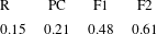
are shown in table 1 for each turbine, calculated from a least square fit of the data in figure 6. The value differs for each case, suggesting that the exponent
 $a$
is not ‘universal’, but rather impeller dependent. This could possibly be due to the fact that
 $a$
expresses how much each impeller type departs from the ‘ideal’ impeller (in the sense that its mass flow rate and output angular momentum are not affected by the level of solid-body rotation in the tank), or simply because the assumptions which were performed for the development of the model are valid to a different extent for each impeller type. In that case, the exponent
 $a$
would effectively act as a fitting coefficient in order to account for the inaccuracy of the model and would depend not only on the impeller type, but on all the geometrical parameters of the configuration.
Optimal value of the exponent
 $a$
, calculated from a least square fit of the data in figure 6, for each turbine type.

For the validation of (2.17) it is necessary to measure the mean fluid velocity in between the blades during a steady-state operation. Ideally, this would require complicated velocity measurements. A qualitative but simpler alternative is the following: first, the impeller’s torque is monitored during an abrupt decrease of shaft speed from a steady state of
 $N_{0}$
Hz, to a smaller speed of
 $N_{2}$
Hz. This enables the measurement of the shaft torque immediately after the deceleration. The above procedure is repeated for different pairs of starting,
 $N_{0}$
, and end speeds,
 $N_{2}$
. Then, using linear interpolation of the data we may determine for every starting speed,
 $N_{0}$
, the necessary end speed,
 ${\tilde{N}}_{2}$
, so that the torque immediately after the deceleration takes zero value. This end speed is approximately the mean fluid velocity in between the blades, i.e.
 $N_{w}={\tilde{N}}_{2}$
.
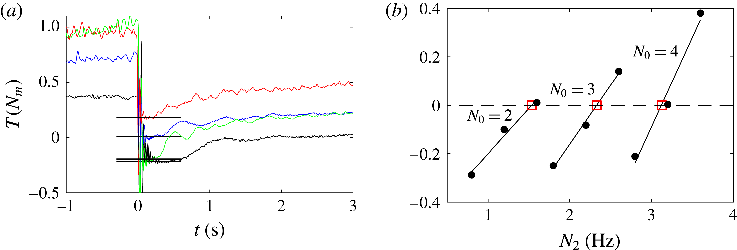
The above torque measurements were performed for the R and PC impellers. Unlike the cases of speed increase, strong blade vibrations were present immediately after decelerating the impeller, contaminating the signal, especially for the cases where the torque approached the zero value after the deceleration. Examples of this can be seen in figure 7(a). For this reason, the acquisition frequency was set to 1 kHz so that the torque values after the deceleration could be determined as accurately as possible. A low pass filter with a cutoff frequency of 100 Hz was used to reduce noise. Examples of the measured torque values immediately after the deceleration for different pairs of
 $N_{0}$
and
 $N_{2}$
can be seen in figure 7(b). As described above, linear interpolation was performed (solid lines) to determine
 $N_{w}$
for each
 $N_{0}$
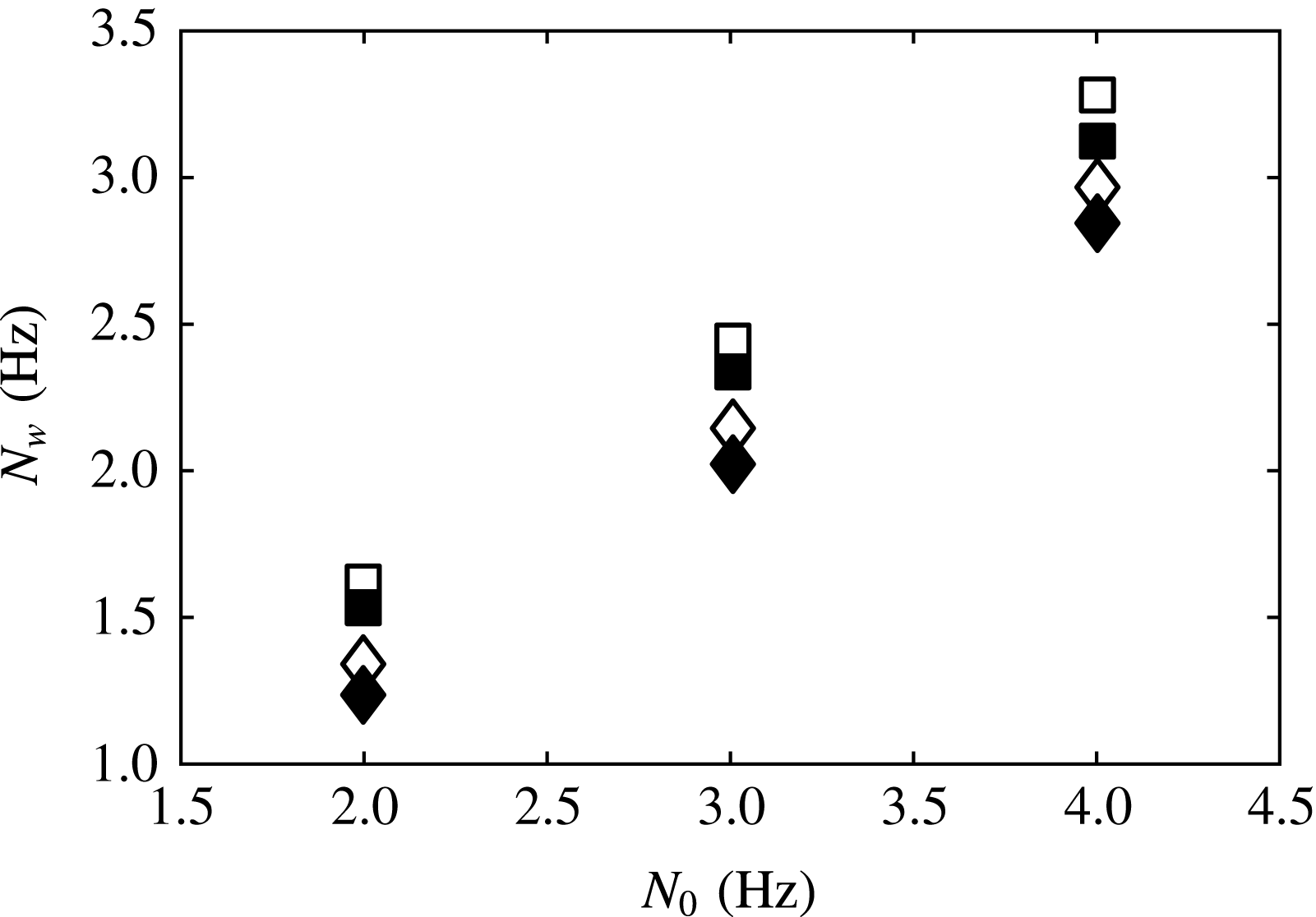
. In figure 8 the values of
 $N_{w}$
are plotted, determined with the experimental method described above, along with the predictions of (2.17), with
 $a$
taken from table 1. For both blade types the predictions agree qualitatively with the measurements, with a maximum overestimation of 8 %.
Example of the measurement method of
 $N_{w}$
for the R impeller: first, the plateau in torque after a sharp deceleration from various steady-state shaft speeds
 $N_{0}$
to given end speeds
 $N_{2}$
is measured (figure 7
a). Then, the necessary shaft speed to achieve
 $T=0$
, i.e.
 $N_{w}$
, is found using linear interpolation for each
 $N_{0}$
(red squares in figure 7(b). (a) Examples of the torque signal after instant decelerations. The thick horizontal black lines are the determined values for each case. (b) Measured plateau torque immediately after a deceleration from
 $N_{0}$
to
 $N_{2}$
. Solid lines: linear fits for each
 $N_{0}$
case. Red squares:
 $N_{2}=N_{w}$
.


3 Transient power number during a quasi-stationary regime
We now model the power number of the impeller–tank system during a transient process. This is done by simplifying the terms of the following expression, derived by angular-momentum balance in the whole tank volume, i.e.
 $$\begin{eqnarray}\frac{\text{d}L_{T}}{\text{d}t}=T_{imp}-T_{w},\end{eqnarray}$$
where
 $L_{T}=\langle \int _{V}r\unicode[STIX]{x1D70C}u_{\unicode[STIX]{x1D719}}\,\text{d}V\rangle$
is the ensemble-averaged (i.e. averaged over many realisations) total angular momentum in the tank and
 $T_{w}$
is the ensemble-averaged wall torque.
3.1 Quasi-steady transition
Equation (3.1) can be simplified under the assumption of quasi-stationarity: in a transient process the impeller adds angular momentum to the fluid, while the wall removes angular momentum from it. In other words, during a time
 $\unicode[STIX]{x1D6FF}t$
there is an increase (or decrease) of
 $L_{T}$
equal to
 $(T_{imp}-T_{w})\unicode[STIX]{x1D6FF}t$
. We now assume that instead of a smooth change of
 $L_{T}$
with time, its change happens in steps which occur with a period of
 $\unicode[STIX]{x1D6FF}t_{s}$
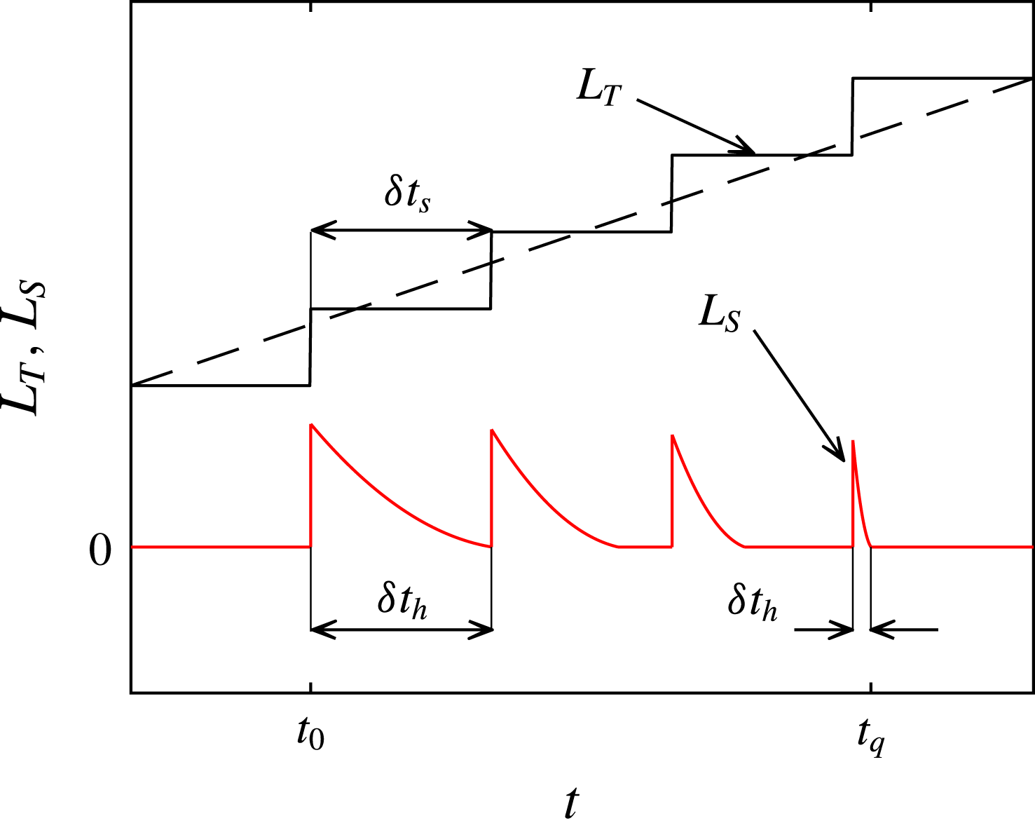
seconds (see cartoon of figure 9). From the above, at
 $t+\unicode[STIX]{x1D6FF}t_{s}$
there is a surplus (or deficit) of angular momentum compared to the previous state, equal to
 $(T_{imp}-T_{w})\unicode[STIX]{x1D6FF}t_{s}$
, which needs to be distributed/homogenised throughout the tank. We may monitor the progress of this ‘homogenisation’ with the parameter (see cartoon of figure 9)
 $L_{S}=\int _{V}\langle \unicode[STIX]{x1D70C}ru_{\unicode[STIX]{x1D719}}-\unicode[STIX]{x1D70C}r\tilde{u} _{\unicode[STIX]{x1D719}}|_{L_{T}}\rangle ^{2}\,\text{d}V$
, where
 $\langle \tilde{u} _{\unicode[STIX]{x1D719}}|_{L_{T}}\rangle$
is the ensemble-averaged tangential velocity distribution corresponding to the particular steady state in which the total ensemble-averaged angular momentum in the tank is
 $L_{T}$
. We assume that the time needed for the difference in angular momentum to be homogenised (i.e. for
 $L_{S}$
to become zero) is
 $\unicode[STIX]{x1D6FF}t_{h}$
. If
 $\unicode[STIX]{x1D6FF}t_{s}>\unicode[STIX]{x1D6FF}t_{h}$
, then, for
 $\unicode[STIX]{x1D6FF}t_{s}-\unicode[STIX]{x1D6FF}t_{h}$
seconds during each period
 $\unicode[STIX]{x1D6FF}t_{s}$
the flow is stationary, and the tangential velocity is given by
 $\langle u_{\unicode[STIX]{x1D719}}\rangle =\langle \tilde{u} _{\unicode[STIX]{x1D719}}|_{L_{T}}\rangle$
. If
 $\unicode[STIX]{x1D6FF}t_{h}/\unicode[STIX]{x1D6FF}t_{s}\ll 1$
then we refer to the flow as being quasi-stationary, i.e. at every moment the ensemble-averaged solid-body rotation is identical to the ensemble-averaged solid-body rotation of a given steady state.
Hypothetical evolution of
 $L_{T}$
and
 $L_{S}$
after an increase of shaft speed. Dashed line: ‘actual’ continuous increase of
 $L_{T}$
. Solid black line: increase of
 $L_{T}$
in steps with a period of
 $\unicode[STIX]{x1D6FF}t_{s}$
seconds. Solid red line: evolution of
 $L_{S}$
with time.
 $\unicode[STIX]{x1D6FF}t_{h}$
is the time needed for the surplus angular momentum to be distributed throughout the tank.
 $t_{0}$
marks the moment where the shaft speed increases, and
 $t_{q}$
the onset of the quasi-steady regime.

In the impeller–tank system we assume that if a deviation from an equilibrium point (
 $\text{d}L_{T}/\text{d}t=0$
) happens at
 $t=t_{0}$
, the flow becomes quasi-stationary at
 $t>t_{q}$
. Then, for
 $t>t_{q}$
, at any given instant the impeller rotates at a speed of
 $N_{2}$
Hz, while the instantaneous ensemble-averaged tangential velocity corresponds to the steady state of an (arbitrary) impeller speed of
 $N_{1}$
Hz which we refer to as the quasi-steady shaft speed. Note that the subscripts
 $1$
and
 $2$
refer to the shaft speed where a quantity was evaluated, and in the case of non-dimensional quantities, with which shaft speed it was normalised.
3.2 Formulation of the equation
We now attempt to simplify each of the terms of (3.1) separately. Assuming a quasi-steady regime, the impeller torque term in (3.1),
 $T_{imp}$
, can be simplified in the following way: first, we note that at any given instant the flow field corresponds to a steady-state solid-body rotation of shaft speed
 $N_{1}$
, while the shaft rotates with a shaft speed
 $N_{2}$
. We may therefore model the instantaneous impeller power number as the value immediately after an impulsive change of shaft speed from
 $N_{1}$
to
 $N_{2}$
Hz, i.e. with (2.19) (where instead of the index 0 we have 1). In the special case where the instantaneous impeller speed is larger than the instantaneous mean fluid speed in between the blades, i.e.
 $N_{2}>N_{w}$
, and considering that since we have assumed a quasi-stationary flow, the solid-body rotation is developed, i.e.
 $N_{1}>0$
, we have for the instantaneous non-dimensional torque (i.e. power number)
 $Np_{2}=(2\unicode[STIX]{x03C0}/\unicode[STIX]{x1D70C}N_{2}^{2}D^{5})T_{imp}$
 $$\begin{eqnarray}\frac{2\unicode[STIX]{x03C0}}{\unicode[STIX]{x1D70C}N_{2}^{2}D^{5}}T_{imp}=\frac{1}{R_{\infty 1}}\left[Np_{\infty 1}^{1/(1+a)}-(Np_{\infty 1}^{1/(1+a)}-Np_{s1}^{1/(1+a)})\frac{N_{1}}{N_{2}}\right]^{1+a},\end{eqnarray}$$
where
 $R_{\infty 1}=Np_{\infty 1}/Np_{\infty 2}$
.
Second, the inertial term,
 $\text{d}L_{T}/\text{d}t$
, can be modelled in a quasi-stationary regime by assuming that the tangential velocity distribution is given by the Rankine vortex profile (
 $\langle u_{\unicode[STIX]{x1D719}}\rangle =\unicode[STIX]{x1D6FA}r$
if
 $r<R_{c}$
and
 $\langle u_{\unicode[STIX]{x1D719}}\rangle =\unicode[STIX]{x1D6FA}R_{c}^{2}/r$
if
 $r\geqslant R_{c}$
, see § 2.1). Then, the instantaneous ensemble-averaged flow field is characterised by a Rankine vortex flow corresponding to the quasi-steady shaft speed
 $N_{1}$
. Considering a cylindrical vessel with radius
 $R_{T}$
and height
 $H$
we obtain
 $$\begin{eqnarray}L_{T}=\left\langle \int _{V}r\unicode[STIX]{x1D70C}u_{\unicode[STIX]{x1D719}}\,\text{d}V\right\rangle =2\unicode[STIX]{x03C0}H\unicode[STIX]{x1D70C}\left(\int _{0}^{R_{c}}\unicode[STIX]{x1D6FA}_{1}r^{3}\,\text{d}r+\int _{R_{c}}^{R_{T}}\unicode[STIX]{x1D6FA}_{1}R_{c}^{2}r\,\text{d}r\right).\end{eqnarray}$$
We further assume that in the impeller inlet (
 $S_{in}$
in figure 1), the contribution of the cross-term
 $\langle u_{n}^{\prime }u_{\unicode[STIX]{x1D719}}^{\prime }\rangle$
is very small when calculating
 $l_{in}$
, and can be therefore neglected. This assumption is realistic for transitional and turbulent unbaffled tanks, as discussed in § 2.1. We may therefore use (2.6), i.e.
 $l_{in1}=R_{c}^{2}/R^{2}$
. Then, from (3.3) we obtain
 $$\begin{eqnarray}\frac{2\unicode[STIX]{x03C0}}{\unicode[STIX]{x1D70C}N_{2}^{2}D^{5}}\frac{\text{d}L_{T}}{\text{d}t}=\frac{1}{N_{2}^{2}}\frac{\text{d}(IN_{1})}{\text{d}t},\end{eqnarray}$$
where
 $I=(\unicode[STIX]{x03C0}^{3}/8)H/R[(R_{T}/R)^{2}-(l_{in1})/2]l_{in1}$
is a moment of inertia dependent coefficient.
 $l_{in1}$
can be calculated by writing (2.10) for the case of the steady state corresponding to
 $N_{1}$
, i.e.
 $Np_{s1}=Np_{\infty 1}(1-l_{in1})^{1+a}$
. In that case
 $I$
becomes
 $$\begin{eqnarray}I=\frac{\unicode[STIX]{x03C0}^{3}}{8}\frac{H}{R}\left\{\left(\frac{R_{T}}{R}\right)^{2}-\frac{1}{2}\left[1-\left(\frac{Np_{s1}}{Np_{\infty 1}}\right)^{1/(1+a)}\right]\right\}\left\{1-\left(\frac{Np_{s1}}{Np_{\infty 1}}\right)^{1/(1+a)}\right\}.\end{eqnarray}$$
Finally, we model the wall torque term in (3.1),
 $T_{w}$
. Since we have considered a quasi-stationary flow, the ensemble-averaged instantaneous transient solid-body rotation in the tank is assumed identical to the ensemble-averaged solid-body rotation corresponding to a steady state of shaft speed equal to
 $N_{1}$
Hz. We now assume that the wall torque is mainly due to the friction caused by the interaction of the solid-body rotation with the wall. Therefore, we may conclude that the instantaneous, ensemble-averaged wall torque is equal to the ensemble-averaged steady wall torque corresponding to an impeller rotating at a speed of
 $N_{1}$
Hz. Then, since in the steady state the wall torque equals the impeller torque we have
 $T_{w}=T_{s1}$
, or
 $$\begin{eqnarray}\frac{2\unicode[STIX]{x03C0}}{\unicode[STIX]{x1D70C}N_{2}^{2}D^{5}}T_{w}=Np_{s1}\left(\frac{N_{1}}{N_{2}}\right)^{2}\end{eqnarray}$$
given that
 $Np_{s1}=(2\unicode[STIX]{x03C0}/\unicode[STIX]{x1D70C}N_{1}^{2}D^{5})T_{s1}$
. Substituting equations (3.2), (3.4) and (3.6) into (3.1) we have
 $$\begin{eqnarray}\frac{1}{N_{2}^{2}}\frac{\text{d}(IN_{1})}{\text{d}t}=\frac{1}{R_{\infty 1}}\left[Np_{\infty 1}^{1/(1+a)}-(Np_{\infty 1}^{1/(1+a)}-Np_{s1}^{1/(1+a)})\frac{N_{1}}{N_{2}}\right]^{1+a}-Np_{s1}\left(\frac{N_{1}}{N_{2}}\right)^{2},\end{eqnarray}$$
which describes the evolution of the quasi-steady speed,
 $N_{1}(t)$
. The unknown functions
 $Np_{s}(Re)$
and
 $Np_{\infty }(Re)$
and the unknown exponent
 $a$
have already been determined experimentally from torque measurements (see § 2.4). Knowing these, along with the geometrical parameters in the tank enables us to solve (3.7) numerically. Then, in conjunction with (3.2), we can have an estimation of the evolution of the transient impeller power number in a stirred tank. Below we summarise all necessary assumptions for (3.7) to be valid. To these we have to add the necessary assumptions for (2.19) to be valid (see § 2.3).
-
(i) The steady-state tangential velocity is modelled by the Rankine vortex profile.
-
(ii) The transition is quasi-steady.
-
(iii) The cross-term
$\langle u_{n}^{\prime }u_{\unicode[STIX]{x1D719}}^{\prime }\rangle$
is negligible in the impeller inlet region (
$S_{in}$
in figure 1), when calculating
$l_{in}$
. -
(iv) The impeller rotates faster than the fluid in the tank (
$N_{2}>N_{w}$
). -
(v) The wall torque is mainly due to the solid-body rotation - wall interaction.
-
(vi) The tank is cylindrical.


3.3 Impulsive shaft speed change by a small amount
In the case where, starting from a steady state of shaft speed
 $N_{0}$
, at
 $t=0$
we impulsively increase the speed to
 $N_{2}~\text{Hz}$
, where
 $N_{2}\rightarrow N_{0}$
, equation (3.7) accepts an analytical solution under the following further assumptions. First, we assume that
 $Np_{\infty }=\text{const.}$
(and
 $R_{\infty 1}=1$
), i.e. a turbulent regime. Second, we assume that
 $l_{in}=\text{const.}$
(i.e. the solid-body rotation does not expand) and thus, from (2.10) we have
 $Np_{s}=\text{const}$
. This assumption is valid in the turbulent regime, as there, the
 $Np_{s}$
of unbaffled tanks drops very weakly with
 $Re$
(Nagata Reference Nagata1975; Steiros et al.
Reference Steiros, Bruce, Buxton and Vassilicos2017b
) and we have assumed an infinitesimal shaft speed (and therefore
 $Re$
) change. In that case (3.7) becomes
 $$\begin{eqnarray}\frac{I}{Np_{\infty }}\frac{\text{d}N^{\ast }}{\text{d}t^{\ast }}=[1-(1-\unicode[STIX]{x1D6FD}^{1/(1+a)})N^{\ast }]^{1+a}-\unicode[STIX]{x1D6FD}{N^{\ast }}^{2},\end{eqnarray}$$
where
 $t^{\ast }=N_{2}t^{\ast }$
is the number of impeller rotations,
 $N^{\ast }=N_{1}/N_{2}$
and
 $\unicode[STIX]{x1D6FD}=Np_{s}/Np_{\infty }$
. Since
 $N^{\ast }\rightarrow 1$
, we can drop the nonlinearity of (3.8) by linearising it around its equilibrium point
 $N^{\ast }=1$
. In that case (3.8) becomes
 $$\begin{eqnarray}\frac{I}{Np_{\infty }}\frac{\text{d}N^{\ast }}{\text{d}t^{\ast }}=[\unicode[STIX]{x1D6FD}^{a/(1+a)}(a+1)-\unicode[STIX]{x1D6FD}(a-1)](1-N^{\ast }).\end{eqnarray}$$
Solving (3.9) we obtain the following expression for
 $N_{2}-N_{1}$
:
 $$\begin{eqnarray}\frac{N_{2}-N_{1}}{N_{2}-N_{0}}=\text{e}^{-t/\unicode[STIX]{x1D70F}}\end{eqnarray}$$
i.e. an exponential decay with a characteristic spin-up time
 $$\begin{eqnarray}\unicode[STIX]{x1D70F}=\frac{I}{N_{2}Np_{\infty }[\unicode[STIX]{x1D6FD}^{a/(1+a)}(a+1)-\unicode[STIX]{x1D6FD}(a-1)]}.\end{eqnarray}$$
We may gain more insight regarding the spin-up time if we express (3.11) for the two limiting cases, i.e.
 $a=0$
and
 $a=1$
(see §§ 2.2 and 2.4). In that case, the non-dimensional spin-up time becomes
 $$\begin{eqnarray}\displaystyle N_{2}\unicode[STIX]{x1D70F} & = & \displaystyle \frac{I}{Np_{\infty }+Np_{s}}\end{eqnarray}$$
 $$\begin{eqnarray}\displaystyle N_{2}\unicode[STIX]{x1D70F} & = & \displaystyle \frac{I}{2(Np_{\infty }Np_{s})^{1/2}},\end{eqnarray}$$
 $a=0$
and
 $a=1$
respectively. It is now clear that the non-dimensional spin-up time is proportional to the moment of inertia-like coefficient,
 $I$
, (which depends on the size of the tank, among others), and inversely proportional to a characteristic power number of the transition, involving both the steady-state and the infinite medium power numbers, which represents the rate angular momentum is being pumped in the tank. In the extreme cases of
 $a=0$
and
 $a=1$
the characteristic power number becomes an arithmetic and a geometric average, respectively. In appendix A (3.12a
) and (3.12b
) are compared with the characteristic spin-up time scale associated with Ekman pumping.
3.4 Experimental validation
Torque experiments were conducted in the stirred tank of figure 3 for the regular impeller only. The acquisition frequency was set to 25 Hz. The power number predictions of (3.7) and (3.2) were validated for three different cases. First, in the late transition after an impulsive increase of shaft speed when the fluid in the tank is quiescent. Second, by varying the shaft speed with a triangular function and third, by varying the shaft speed with a sinusoidal function.
Particular attention should be paid to the shape of the tank, as it is octagonal (see figure 3) and not the conventional cylindrical, a fact which could possibly affect the validity of (3.7). Specifically, angles/corners in the tank shape create recirculation zones which could potentially destroy the statistical axisymmetry of the flow. As these zones expand, they progressively create a ‘baffling’ effect, i.e. they increase the steady-state power number and break the solid-body rotation (see Steiros et al.
Reference Steiros, Bruce, Buxton and Vassilicos2017b
; Myers, Reeder & Fasano Reference Myers, Reeder and Fasano2002). The above become more pronounced as the wall angles become more acute. Therefore, in our case of considerably obtuse angles we could assume that the recirculation regions are confined in the vicinity of the tank corners and that the statistical axisymmetry is retained in a cylinder of radius equal to the inner radius of the octagon,
 $R_{T}$
. This cylinder size is used henceforth when calculating the various terms of (3.7). A way to test the sensitivity of the flow field to the wall angles is to compare the steady-state power number produced by an octagonal tank, with the two extreme cases: a cylindrical unbaffled tank with an axisymmetric solid-body rotation (no baffling effect), and a cylindrical baffled tank in which the solid-body rotation is almost non-existent (large baffling effect). As shown in Steiros et al. (Reference Steiros, Bruce, Buxton and Vassilicos2017b
), when considering a flat-blade impeller and a turbulent regime, insertion of baffles in a cylindrical tank increases the power number by over four times, whereas if the tank remains unbaffled, but its shape changes to octagonal, the power number increases by approximately 35 %. This suggests a close resemblance of the octagonal and cylindrical tanks’ flow fields.
3.4.1 Late transition after an impulsive increase in shaft speed
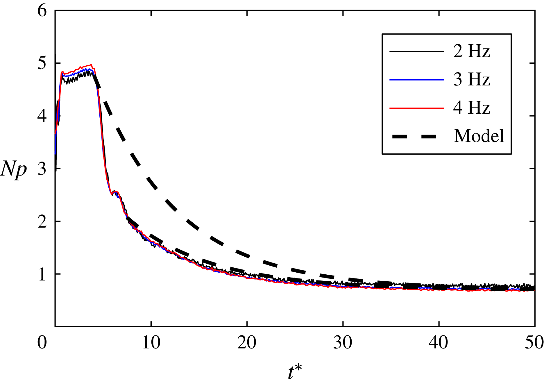
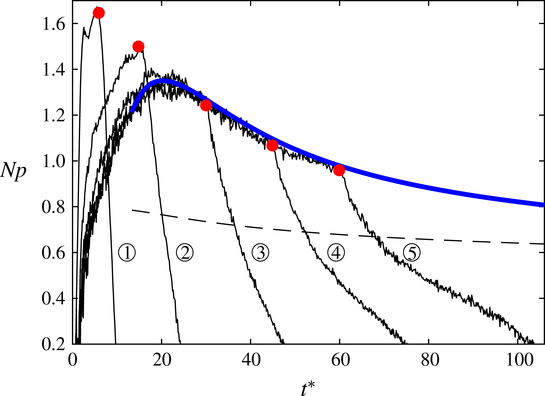
Three end-shaft speeds were investigated, i.e. 2, 3 and 4 Hz. The impeller starting speed was zero in all cases. The experiments were repeated ten times for each case, and ensemble averaging was performed to reduce the signal fluctuations. In figure 10 the measured ensemble-averaged power numbers,
 $Np$
, are plotted over the number of impeller rotations,
 $t^{\ast }=tN_{2}$
, for the three different end speeds. The power numbers exhibit a plateau (
 $t^{\ast }<5$
), then an abrupt drop, and finally reach the steady state (
 $t^{\ast }>40$
), in accordance with the observations of Maynes & Butcher (Reference Maynes and Butcher2002). We observe a good collapse between the three curves, suggesting a self-similarity of the flow fields. In the plateau and steady-state regions the curves deviate from each other slightly, suggesting a small
 $Re$
dependence, consistent with earlier remarks (see § 2.4).
In figure 10 the numerical solution of (3.2) and (3.7) is also plotted, using
 $a=0.15$
, which is the optimal exponent for the R impeller, as shown in § 2.4. The model’s starting point was chosen after the abrupt drop in power number (
 $t^{\ast }=7.5$
), i.e. after the discharged fluid has recirculated back to the impeller region, as the flow cannot not be quasi-stationary before this point. As shown in the plot, good agreement is achieved between the prediction and the measurements.
Ensemble-averaged power numbers after impulsive changes of shaft speed, over the number of impeller rotations
 $t^{\ast }$
. Solid lines: measurements, from
 $N_{0}=0$
to different end speeds,
 $N_{2}$
, as shown in the legend. Dashed black line: numerical solution of (3.7) and (3.2), starting at the late transition (
 $t^{\ast }=7.5$
).

3.4.2 Triangular and sinusoidal variation of the shaft speed
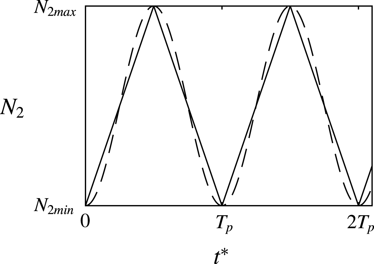
The shaft speed was varied using a triangle and a sinusoidal function, always between a minimum shaft speed
 $N_{2min}=1~\text{Hz}$
and a maximum shaft speed
 $N_{2max}=5~\text{Hz}$
(see figure 11). Experiments were performed for five wave period values, i.e.
 $T_{p}=$
4, 10, 20, 30 and 40 s, to examine the sensitivity of the quasi-steady region to the impeller acceleration. Measurements were conducted for a few periods before recording, so that initial phenomena had subsided. Phase averaging was then performed over several periods to reduce signal fluctuations due to measurement errors and turbulence. Note that since the experimental conditions did not differ from one period to another, phase averaging was equivalent to ensemble averaging.
Types of time varying shaft speeds used in the experiments:
 $N_{2min}=1~\text{ Hz}$
;
 $N_{2max}=5~\text{Hz}$
;
 $T_{p}\in \{4,10,20,30,40\}~\text{s}$
. Dashed line: sinusoidal wave. Solid line: triangle wave.

Ensemble-averaged power numbers over the number of impeller rotations. Solid black lines: measurements corresponding to the triangle speed variation. 1:
 $T_{p}=4~\text{s}$
, 2:
 $T_{p}=10~\text{s}$
, 3:
 $T_{p}=20~\text{s}$
, 4:
 $T_{p}=30~\text{s}$
, 5:
 $T_{p}=40~\text{s}$
. Solid blue line: prediction using (3.7) and (3.2) for a steady acceleration equal to the
 $T_{p}=40~\text{s}$
cases. Dashed black line: steady-state power number of the same instantaneous shaft speed as the prediction’s (blue line). Red points: end of shaft acceleration - start of shaft deceleration for the measurements.

Ensemble-averaged power numbers versus the number of impeller rotations for triangle and sinusoidal wave variation of the shaft speed (see figure 11). Black solid lines: measurements. Red lines: predictions using (3.2) and (3.7). Dashed lines: predictions using (3.2), assuming
 $N_{1}=$
const. Blue line: prediction using (3.7) and (3.2) starting from a wrong initial condition. The white regions signify the acceleration branches of the waves, while the gray regions the deceleration branches.

In figure 12 the measured ensemble-averaged shaft power numbers corresponding to the triangle case are plotted versus the number of shaft rotations
 $t^{\ast }=\int N_{2}\,\text{d}t$
(
 $t^{\ast }=0$
corresponds to the start of the wave’s acceleration branch). We observe that the accelerating branches of the signals corresponding to
 $T_{p}\geqslant 20~\text{s}$
collapse, suggesting self-similarity of their flow fields, while for smaller period values the signals deviate, presumably because the fluid in the tank does not respond in the same way to the shaft acceleration and self-similarity is lost. The prediction of (3.7) and (3.2) using
 $a=0.15$
is also plotted in figure 12 with the solid blue line, for a constant steady acceleration of the shaft, corresponding to the accelerating branch of the triangle function of
 $T_{p}=40~\text{s}$
, i.e.
 $\text{d}N_{2}/\text{d}t=0.2~\text{s}^{-2}$
. The prediction follows very well the measurements, showing that the underlying assumptions of (3.7) are valid in this region. For very large
 $t^{\ast }$
the prediction tends asymptotically to the steady-state power number of shaft speed equal to the prediction’s (calculated by extrapolating the measured values of figure 6
a). This suggests that if a steady shaft acceleration is performed for a large number of shaft rotations, the flow effectively ‘catches up’ with the impeller.
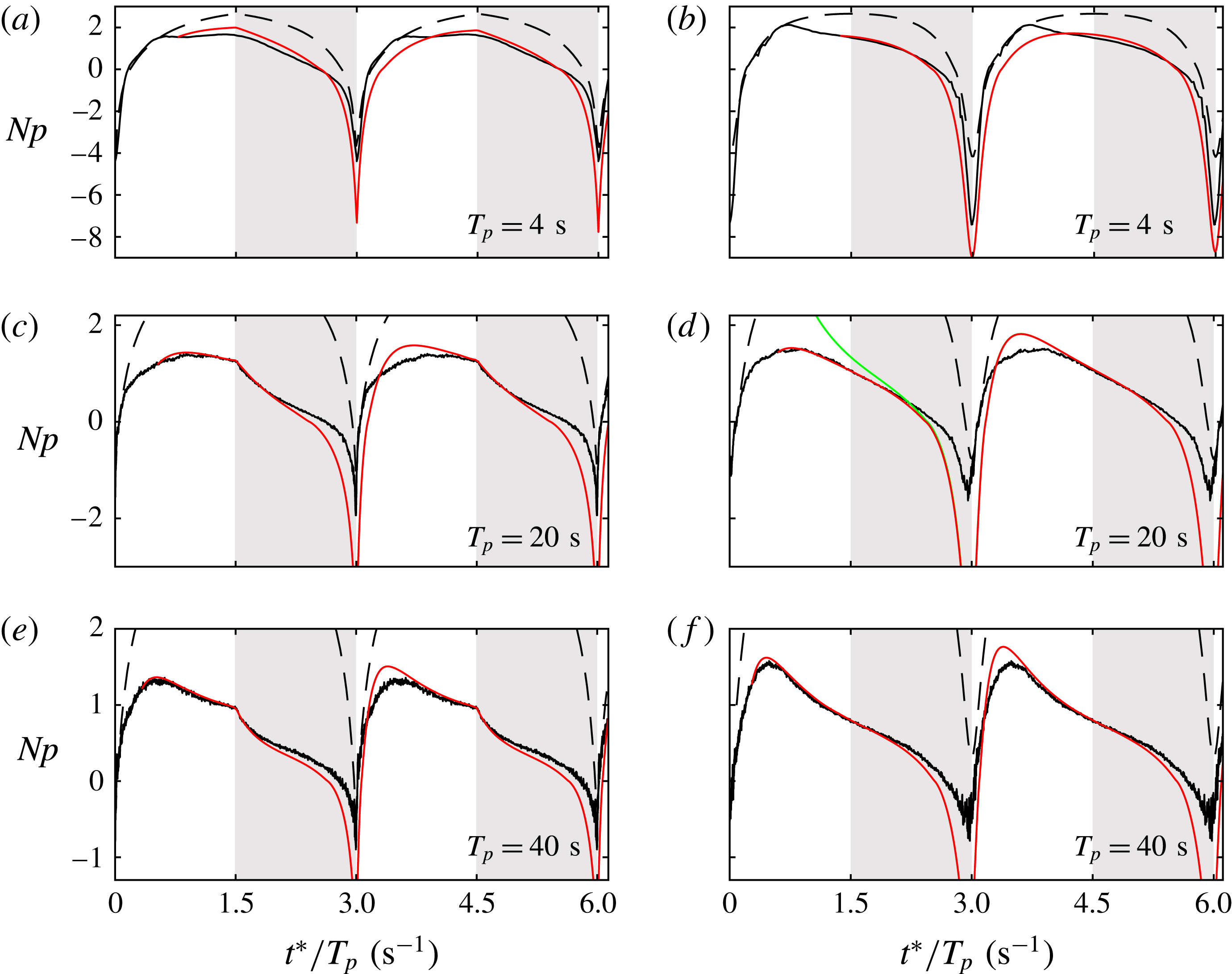
In figure 13 the measured ensemble-averaged power numbers of the triangle and sinusoidal speed waveforms are plotted over the number of shaft rotations divided by
 $T_{p}$
, spanning 2.1 wave periods. Only the cases of
 $T_{p}=4$
, 20 and 40 s are presented. The predictions of (3.7) and (3.2) are also plotted for
 $a=0.15$
. For both waveforms we observe that the predictions and measurements agree best around the wave peak; this is still quite poor for
 $T_{p}=4~\text{s}$
, improves for
 $T_{p}=20~\text{s}$
and becomes very good for
 $T_{p}=40~\text{s}$
, as then the impeller speed changes with a slow enough pace for the flow to follow and be considered quasi-stationary. In the deceleration branch of the waves the solution starts to diverge from the measurements: this is expected, since the value
 $a=0.15$
was experimentally determined for shaft accelerations (see § 2.4), and may therefore not be valid for decelerations. Moreover, one of the assumptions for (3.7) to be valid, is that the instantaneous impeller speed is larger than the mean fluid speed between the blades, i.e.
 $N_{2}>N_{w}$
, which requires the power number to be positive (energy being given to the flow rather than being extracted). Therefore, for
 $Np<0$
the predictions cannot be considered valid. The agreement is also inadequate in the start of the acceleration branch, possibly because the flow field has not become quasi-steady yet. It is noteworthy to mention that the prediction is more accurate during the first wave period (
 $t^{\ast }/T_{p}<3~\text{s}^{-1}$
) than during the second one. This is because while the prediction was picked to start from a realistic initial condition, the first deceleration branch causes a large discrepancy between the prediction and the measurements, essentially imposing a wrong initial condition for the second period.
To check the overall sensitivity of the predictions to the initial conditions, a prediction corresponding to
 $a=0.15$
was calculated, but with a wrong initial condition (blue line in figure 13). After some impeller rotations the curves corresponding to wrong and correct initial conditions converge, showing that the model can provide sensible predictions even with arbitrary initial conditions.
Finally, in figure 13 the predictions of the power number of (3.2) are plotted with dashed lines, assuming that the quasi-steady speed,
 $N_{1}$
, stays constant with time, i.e. assuming that the flow does not adapt to the impeller speed change at all. The value which was chosen for
 $N_{1}$
for each case was the one which made these predictions match best with the experiments at the start of acceleration. We observe that for
 $T_{p}=4~\text{s}$
the predictions agree qualitatively with the measurements during the whole wave period, and especially during the first stage of impeller acceleration (
 $t^{\ast }/T_{p}<0.75~\text{s}^{-1}$
) they collapse with the data. This suggests that for such small wave period values the fluid cannot effectively respond to the changes in the speed of the impeller. For the larger
 $T_{p}$
cases, the agreement of the
 $N_{1}=\text{const.}$
predictions with the measurements becomes unrealistic. This signifies that the impeller now accelerates slow enough for the flow to adapt.
4 Discussion
4.1 Power number drop in unbaffled tanks at turbulent conditions
Equation (2.10), which models the dependence of the power number on the solid-body rotation, can help us draw qualitative conclusions regarding the behaviour of the steady-state power number of unbaffled stirred tanks at turbulent conditions. In the steady state the impeller torque equals the torque exerted on the tank wall by the fluid. In that case we have
 $$\begin{eqnarray}\displaystyle Np_{s} & = & \displaystyle Np_{\infty }(1-l_{in})^{1+a},\end{eqnarray}$$
 $$\begin{eqnarray}\displaystyle Np_{s} & = & \displaystyle C_{w}\left(\frac{U_{w}}{\unicode[STIX]{x03C0}DN}\right)^{2}.\end{eqnarray}$$
 $C_{w}$
is a skin friction-like coefficient of the wall, while
 $U_{w}/\unicode[STIX]{x03C0}DN$
is the non-dimensional mean tangential velocity near the wall due to the solid-body rotation. The latter is an increasing function of
 $l_{in}$
, as can be readily verified if we model the tangential velocity distribution in the tank as a Rankine vortex.
It has been experimentally observed that the steady-state power number of unbaffled tanks drops with
 $Re$
for the highly turbulent regime (see for instance Nagata (Reference Nagata1975), Steiros et al. (Reference Steiros, Bruce, Buxton and Vassilicos2017b
) and Laity & Treybal (Reference Laity and Treybal1957)). Since in that regime
 $Np_{\infty }$
is constant, equation (4.1a
) shows that
 $l_{in}$
must increase, i.e. the ‘extent’ of the solid-body rotation increases in the tank. Equation (4.1b
) shows that this is only possible if the skin friction coefficient of the wall drops (since
 $U_{w}/\unicode[STIX]{x03C0}DN$
is an increasing function of
 $l_{in}$
and
 $Np_{s}$
drops with
 $Re$
). We may therefore interpret the drop of the power number in unbaffled stirred tanks in the turbulent regime in the following way: as
 $Re$
increases, the friction coefficient of the walls,
 $C_{w}$
, drops, in analogy to the flat-plate boundary layer behaviour (Schlichting & Gersten Reference Schlichting and Gersten1979). The impeller–tank system loses then its equilibrium, as the impeller produces more angular momentum than the wall can destroy. As a result, a stronger solid-body rotation/swirl is generated, with larger normalised fluid tangential velocities near the wall,
 $U_{w}/\unicode[STIX]{x03C0}DN$
. We note that the increasing trend of the normalised tangential velocity with
 $Re$
in turbulent unbaffled conditions has been experimentally verified by Yoon et al. (Reference Yoon, Hill, Balachandar, Adrian and Ha2005) and Nagata (Reference Nagata1975). The above results in an increase in wall torque (as the wall velocities increase), and a decrease in impeller torque (as the relative tangential blade velocity decreases). Subsequently, the system reaches a new steady state with a decreased impeller power number. The above occur continuously as
 $C_{w}$
decreases, i.e. as
 $Re$
increases, leading to the documented drop in impeller torque/power number (Nagata Reference Nagata1975; Steiros et al.
Reference Steiros, Bruce, Buxton and Vassilicos2017b
; Laity & Treybal Reference Laity and Treybal1957) and impeller drag (Steiros et al.
Reference Steiros, Bruce, Buxton and Vassilicos2017b
) with increasing
 $Re$
. In baffled vessels on the other hand, the power number is constant in the turbulent regime (Nagata Reference Nagata1975; Laity & Treybal Reference Laity and Treybal1957). From the above discussion this implies that the solid-body rotation and flow field are self-similar in baffled tanks (i.e.
 $l_{in}=\text{const.}$
), something verified by velocity measurements (see for instance Nagata (Reference Nagata1975)).
4.2 Applicability of the models
Equations (2.19) and (3.7), which predict the transient torque of stirred tanks, rely on several assumptions, some of which may not be valid in special cases. It would be therefore useful to investigate the applicability of these models, with respect to the conditions of operation.
It is expected that the models do not hold in the laminar regime, as in that case the necessary condition of a developed solid-body rotation in the tank is not fulfilled (see Nagata Reference Nagata1975). For the same reason, it is expected that the models do not hold, or require a correction, in baffled tanks, as baffles tend to suppress the solid-body rotation in the tank and break the axial symmetry of the flow. Regarding the tank size, a small departure from the ‘standard’ size (see discussion in § 2.1) should not affect the validity of the models, as long as it does not alter the solid-body rotation in the tank, which is assumed to follow a two-dimensional Rankine vortex profile. However, drastic departures from the ‘standard’ size, as for instance very tall/large tanks, could break the two-dimensionality of the solid-body rotation, rendering the models unrealistic. A correction would be needed in such cases.
Another important aspect is the impeller type. An impeller change is expected to cause a change in the coefficient
 $a$
(see § 2.1), which takes into account the change in the impeller pumping. Furthermore, the Rankine vortex profile, which models faithfully the solid-body rotation generated by radial impellers (see Nagata Reference Nagata1975), may not be valid for other impeller types, as for instance axial impellers, where the Rankine vortex requires a correction coefficient to be valid (see Busciglio et al. (Reference Busciglio, Caputo and Scargiali2013)). Such changes need to be taken into account in the formulation of (2.19) and (3.7).
Finally, it is important to discuss the types of speed variation for which (2.19) and (3.7) can provide a sensible torque prediction. It was shown that when considering an impulsive increase in the shaft speed, the models can predict the torque plateau (spike) immediately after the speed increase, as well as the torque during the late transition. In between these two stages, the models are not valid. Regarding smooth variations in the shaft speed, the models were shown to adequately predict the transient torque when the shaft acceleration was picked to be small enough so that the flow can be considered quasi-steady. However, for sharper accelerations the model accuracy considerably declined. When considering shaft decelerations, the models can be considered valid only when the shaft speed remains larger than the mean fluid speed between the blades, as this was one of the assumptions for the formulation of (2.19) and (3.7).
5 Summary
In this article analytical models for the prediction of the transient power number in stirred tanks are developed and experimentally validated using torque measurements.
First, in § 2, a low-order model based on angular-momentum balance in a control volume around the impeller is developed, linking the impeller power number with the parameter
 $l_{in}$
, which describes the ‘extent’ of the fluid solid-body rotation in the tank. This model is subsequently used to predict the power number immediately after an impulsive change in shaft speed. The predictions are then compared with experimental data. Good agreement is found for all tested cases.
Second, in § 3, using angular-momentum balance in the whole tank and the above model, an ordinary differential equation which describes the evolution of the impeller power number in transient conditions, in a quasi-stationary regime, is developed. To solve the above equation the impeller dependent parameters
 $Np_{s}$
,
 $Np_{\infty }$
and
 $a$
are needed, which are easily determined from simple torque experiments, along with the geometrical parameters of the impeller–tank system. For the case of an impulsive change of the shaft speed by a small amount, the equation is shown to have an analytical solution, providing a characteristic spin-up time scale. To validate the models, torque experiments were performed for the case of sinusoidal and triangle wave variation of the shaft speed, as well as impulsive increases of the shaft speed. For all cases the predictions show good agreement with the measurements, when the underlying assumptions are valid.
Finally, using results obtained from the above models, an explanation of the reported drop of power number in unbaffled tanks at high Reynolds numbers is proposed. It is suggested that the drop is linked to the decrease in the friction coefficient of the tank walls with increasing
 $Re$
, similar to a flat-plate boundary layer. Furthermore, the applicability of the models is discussed.
Acknowledgements
This work was supported by the EU through the FP7 Marie Curie MULTISOLVE project (grant agreement no. 317269). The author is very grateful to Professor Christos Vassilicos, Dr Paul Bruce and Dr Oliver Buxton for reading the paper and making helpful suggestions and comments.
Appendix A. Ekman and impeller pumping during spin up
The characteristic spin-up time scale, calculated in § 3.3, naturally depends on the secondary circulatory flows in the tank, which transfer and ‘homogenise’ the angular momentum. The main circulatory motion is due to the impeller rotation, depicted in figure 1. However, another circulatory motion, that of Ekman pumping may be also present, caused by the angular velocity difference between the rotating fluid and the static top–down walls (see Greenspan & Howard Reference Greenspan and Howard1963; Benton & Clark Reference Benton and Clark1974). It would be therefore interesting to compare the Ekman spin-up time scale, with that of the current procedure, which includes the impeller pumping, i.e. (3.12a ) and (3.12b ).
The effect of Ekman pumping has not been established yet for the spin up of a stirred tank, but it has been determined for the simpler case of a rotating tank, performing small or large impulsive changes in its speed, when no impeller is present. If we assume that the results of the rotating tank can be approximately applied to the stirred tank case as well, we may estimate the characteristic spin-up time due to Ekman pumping of a stirred tank as (see Greenspan & Howard Reference Greenspan and Howard1963; Benton Reference Benton1973)
 $$\begin{eqnarray}\unicode[STIX]{x1D70F}_{E}=(d^{2}/\unicode[STIX]{x1D708}\unicode[STIX]{x1D6FA})^{1/2};\end{eqnarray}$$
where
 $d$
is a characteristic length, commonly the tank diameter, i.e.
 $d=D_{T}$
. Considering the water tank of figure 3 and for the case of a fluid rotating at an angular velocity of
 $N=5~\text{Hz}$
, equation (A 1) yields an Ekman spin-up time of
 $\unicode[STIX]{x1D70F}_{E}\approx 80~\text{s}$
, whereas the characteristic spin up involving an impeller rotating at
 $N=5~\text{Hz}$
can be calculated using either (3.12a
) or (3.12b
) as
 $\unicode[STIX]{x1D70F}\approx 2~\text{s}$
, i.e. an order of magnitude smaller. The above suggests that impeller pumping is much more important compared to Ekman pumping in the spin up of turbulent stirred tanks. This is because an impeller generally pumps much more efficiently compared to an Ekman layer: in the case of a turbulent tank stirred by a radial impeller rotating at an angular frequency
 $\unicode[STIX]{x1D6FA}$
, pumping velocity (i.e. radial velocity in the discharged region of the impeller) is of the order of
 $U/\unicode[STIX]{x1D6FA}R=O(10^{-1})$
(see Yoon et al. (Reference Yoon, Hill, Balachandar, Adrian and Ha2005)). For the case of a static tank with no impeller, in which the fluid performs a solid-body rotation with an angular frequency
 $\unicode[STIX]{x1D6FA}$
, Ekman pumping velocity is approximated as (see Benton & Clark Reference Benton and Clark1974)
 $U_{E}\approx 0.3(\unicode[STIX]{x1D708}\unicode[STIX]{x1D6FA})^{1/2}$
, or equivalently
 $$\begin{eqnarray}\frac{U_{E}}{\unicode[STIX]{x1D6FA}R}\approx 0.25Re^{-1/2},\end{eqnarray}$$
where
 $Re=ND^{2}/\unicode[STIX]{x1D708}$
is the conventional Reynolds number of stirred tanks. Therefore, for a turbulent tank of
 $Re>10\,000$
, Ekman pumping is estimated to be negligible compared to the pumping produced by the impeller.