2. DYNAMIC ORBIT DETERMINATION

The kinematic approach to POD depends entirely on the observational geometry and the GPS signal continuity, thus a purely kinematic solution might not always be of sufficient quality and continuity due to insufficient observations and poor geometric configuration (Byun, Reference Byun2003). In the dynamic POD, however, all forces acting on the satellite are computed, based on the physical principles and models, and integrated numerically to estimate the initial state vector (position and velocity at the initial epoch) along with other unknown parameters, such as the scaling factors for the atmospheric drag and solar radiation pressure.

These parameters are connected to the GPS measurements via the variational partials, therefore the final orbit solution can be improved by estimating these unknown parameters together with the initial state vector. Once the initial state vector and other dynamic parameters are estimated, the state vector for the following epochs can be propagated using the force models used in the estimation process, thus the errors in the dynamic approach will grow as the arc length increases.

In practice, many coefficients for the empirical forces are included in the dynamic orbit determination to absorb the unmodelled forces. Sometimes pseudo-stochastic pulses are set up at the pre-determined epochs and time intervals to introduce the velocity change in a pre-determined direction (Bock, Reference Bock2003).

The equation of motion of the satellite is generally expressed in the Earth Centred Inertial (ECI) frame as follows (Hugentobler et al., Reference Hugentobler, Schaer and Fridez2001):

(1)

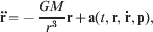
where

r:

3×1 satellite position vector in the inertial frame at time t;

:

total acceleration of the satellite at time t;

GM:

product of the gravitational constant and the mass of the Earth;

r:

magnitude of the position vector r;

a:

total perturbing forces;

t:

time, at which the acceleration is calculated;

ṙ:

velocity of the satellite at time t;

p:

parameter vector, which induces the perturbing acceleration.

The total perturbing forces, a, represent the third-body gravitational forces, atmospheric drag, solar radiation pressure and/or some empirical force terms which normally account for all unmodelled forces, including the nonspherical part of the Earth's gravity field. These perturbing forces as well as the Keplerian accelerations are computed at each epoch and then numerically integrated to get the position and velocity of the satellite at that epoch. The obtained position and velocity of the satellite are used to validate the measurements from GPS satellites at the same epoch, and finally update the unknown parameter vector including the initial state vector, as mentioned earlier.

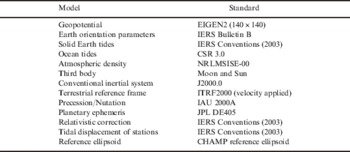
Table 1 shows the summary of the models and the conventions that are related to the perturbing forces and are used in this study. EIGEN2 is the geopotential model, degree and order up to 140, which is generated from six months of CHAMP data only. Solid Earth tides are implemented for both temporal variation of the geopotential coefficients and the displacement of the IGS ground stations based on IERS Conventions (2003). For the ocean tides, CSR 3.0 model obtained from the analysis of TOPEX/POSEIDON altimeter data is used. Only the Moon and the Sun are considered for the third-body perturbations. The equation of motion can be solved by the numerical integration method in the inertial frame, therefore all the coordinates and the force components computed in the terrestrial frame should be transformed into the inertial frame. For this transformation, new IAU 2000A resolutions are used for the precession/nutation model, based on the reference origin at J2000.0. It should be mentioned that the published IGS stations refer to a certain reference epoch, thus the velocity of the station should be applied to compensate for the plate tectonic motion. Since the atmospheric and empirical force modelling is critical in dynamic orbit determination of LEO, theses models are described in detail in the next section.

Table 1.

Summary of the strategies for the dynamic precise orbit determination.

3. ATMOSPHERIC AND EMPIRICAL FORCE MODELLING

While the conservative forces and the tidal variations can be modelled very accurately, the challenge rests in modelling the nonconservative forces, especially atmospheric drag. Atmospheric drag is the most dominant of all nonconservative forces at LEO altitude, which amounts to approximately 1000 m of orbit error after two revolutions (Bae, Reference Bae2005). Accurate modelling of the atmospheric force is not an easy task due to the incomplete knowledge of the physical properties of the atmosphere and the varying attitude of nonspherical, irregularly shaped satellites with respect to the atmospheric particle flux (Montenbruck and Gill, Reference Montenbruck and Gill2001). To make up for this inaccuracy in the atmosphere models, the scaling factors for the atmospheric forces are usually estimated in the orbit determination process.

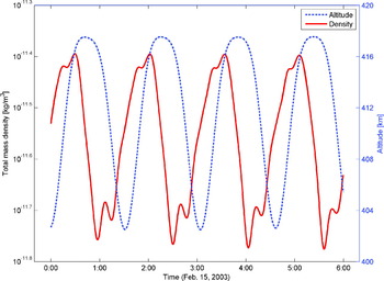
Figure 1 shows the total mass density variation along the CHAMP trajectory using the NRLMSISE-00 (NRL Mass Spectrometer, Incoherent Scatter Radar Extended Model) atmosphere model. This model was developed, based on the satellite mass spectrometer and ground-based incoherent scatter data, to provide a single analytic model for calculating temperature and density profiles (Hedin, Reference Hedin1991). It is a function of many different variables, i.e., local time, latitude, annual/semiannual, and longitude variations. This model is expanded in terms of the lower-order spherical harmonics and the Fourier series with the parameters of the temperature profile and density boundary conditions at 120 km. Thus, it allows for an easy determination of temperature and density profiles for specific geographic and solar/magnetic parameters. It should be noted that the atmospheric density repeats itself for every orbit with a slight change; therefore, the time interval for the estimation of the coefficients is an important issue for the precise orbit determination.

Figure 1.

Atmospheric density variation along the CHAMP trajectory based on NRLMSISE-00.

The atmospheric drag can be modelled using the well-known equation (Montenbruck and Gill, Reference Montenbruck and Gill2001)

(2)

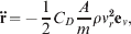
where m is the mass of the spacecraft; C _D is the drag coefficient which is a dimensionless quantity describing the interaction of the atmosphere with the satellite's surface material; ρ is the density of the atmosphere; A is the area of the satellite surface perpendicular to the satellite velocity; v_r is the velocity of the object relative to the atmosphere

(3)

and its unit vector and the magnitude is given by

(4)

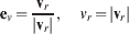
with the velocity vector v and the position vector r of the satellite in the inertial frame, and the Earth angular velocity vector ω.

The drag coefficient, C _D, known also as the scaling factor, is used to compensate the incomplete density model; therefore, it is the primary unknown in the LEO dynamic orbit determination. The partial derivatives of the acceleration with respect to the drag coefficient, C _D, consist of two parts, as shown in Equation (5):

(5)

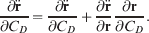
The explicit component of the partial derivatives (first term on the right side of Equation (5)) can be easily computed from Equation (2). The implicit component, however, requires a numerical integration of Equation (5) up to the current epoch. It should be mentioned that the density variation is not so sensitive to the positional change because the density is a small value compared to the magnitude of the position vector, and changes very smoothly at the CHAMP altitude, as can be seen in the density model.

Another important parameterization is the empirical force modelling. Although a considerable number of orbit errors can be removed through the estimation of the atmospheric drag coefficients, as explained above, there still remains an unmodelled force. Therefore, it is impossible to model the forces acting on the satellite in a true and pure dynamic approach. This can be dealt with as empirical force modelling, depending on the frequencies to be modelled. Since the unmodelled force has periodic properties, once-per-revolution and possibly twice-per-revolution components are usually modelled in the dynamic POD approach. Due to the dynamic coupling between the along-track and the radial components, only the cross-track and the along-track components are modelled to avoid ill-conditioning the system (Boomkamp, 2004, personal communication). The once-per-revolution empirical force in RTN (Radial, Transverse and Normal) frame can be modelled as a sum of the sine and the cosine terms in each direction as follows:

(6)

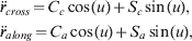
where

C _c,S _c,C _a,S _a:

coefficients of the sine and the cosine terms in each direction;

u:

argument of latitude of the satellite.

Since the empirical forces are modelled in the RTN frame, these should be transformed into the inertial frame to be combined with the remaining accelerations. This transformation matrix can be computed using the satellite inertial position and velocity, and is given as follows:

(7)

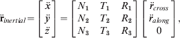
where

(8)

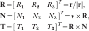
with the position vector r and the velocity vector v of the satellite in the inertial frame.

4. TRIPLE DIFFERENCING TECHNIQUE

The double-differenced (DD) GPS carrier phase measurements are widely used as observables in the orbit determination procedure. This is because, through differencing, most of the error sources are removed, including the GPS satellite and receiver clock errors; moreover, the integer ambiguity fixing provides strong constraints to the positioning solution. In the real applications of the LEO orbit determination however, since the baselines between the tracking stations and LEOs are normally very long (hundreds to thousands of kilometres), it is not easy to resolve the integer ambiguities due to the residual ionospheric effects (Byun and Schutz, Reference Byun and Schutz2001). The reported success rate of the ambiguity resolution is at the level of about 40%, based on fixing the wide-lane ambiguities, and about 18% of the subsequent narrow-lane ambiguities (Švehla and Rothacher, Reference Švehla and Rothacher2003). In addition, the number of unknown ambiguities account for most of the unknown parameters in the double-difference dynamic POD.

In order to avoid the time-consuming and complicated ambiguity resolution process the triple differenced, ion-free, GPS carrier phase data are used as primary observations in this study. The triple differencing technique for orbit determination was first applied for the GPS satellites in a dynamic approach by Grejner-Brzezinska (Reference Grejner-Brzezinska1995), and for the LEO satellites in the kinematic application by Kwon et al. (Reference Kwon, Grejner-Brzezinska, Bae and Hong2003) ; it was also used for the geodetic network adjustment (Eren, Reference Eren1986) or as a priori solution for the double-differenced approach (Byun and Schutz, Reference Byun and Schutz2001). Remondi and Brown (Reference Remondi and Brown2000) present an interesting implementation of triple-differenced carrier phases combined with double-differenced code measurements in a delayed-state Kalman filter in static and dynamic positioning. The most pronounced advantage of the triple differencing technique is that the unknown phase ambiguities are entirely removed; thus the size of the normal equations is significantly decreased while the solution quality is equivalent to the double-difference float solution, as proved by Schaffrin and Grafarend (Reference Schaffrin and Grafarend1986). Besides the removed nuisance parameters, there is no need to detect and correct the cycle slips because these are treated as data outliers and removed during the estimation process by the residual cut-off (threshold) criterion.

In triple differencing, however, the measurement noise is amplified, and the observations are correlated epoch by epoch due to the differencing in time. In addition, the potentially strong constraints coming from the fixed integer ambiguities are lost. However, this disadvantage should be perceived in the context of the relatively low level of reported success in the ambiguity resolution in the double-differencing mode, as already mentioned. Also, the correlation can be resolved by a simple and efficient algorithm, which decomposes the covariance matrix using the Cholesky factorization (Kwon et al., Reference Kwon, Grejner-Brzezinska, Bae and Hong2003). The triple-differenced GPS carrier phase observables are given as follows (Grejner-Brzezinska, Reference Grejner-Brzezinska1995):

(9)

(10)

where

Φ:

GPS carrier phase measurement in distance unit;

ρ:

geometric range between the transmitter and the receiver;

f:

frequency of the carrier phase;

I/f ²:

ionospheric refraction;

T:

tropospheric refraction;

ε:

measurement noise for phase measurement.

Superscripts k and l represent the transmitters (GPS satellites) and subscript i and j represent the receivers; number 1 or 2 in the subscript means that the corresponding term is referred to L1 or L2 signal, respectively; the subscript dt represents the time difference of the consecutive double-differenced observables. The ion-free combination of the triple-differenced GPS carrier phase observables can be written as follows:

(11)

5. PROCESSING STRATEGY AND NUMERICAL TEST

The triple differencing POD approach is designed to compute the orbit solution in near real-time to support the GPS meteorology for atmospheric profiling; thus it is important to satisfy the requirement of the processing efficiency as well as the orbit accuracy. To demonstrate the application of this technique, 26 hours of CHAMP data collected on 15 February 2003 are processed in this study. Usually a 30-hour arc (24 hours of data plus 3 hours of data before and after each day) is used for the LEO dynamic POD to reduce the edge effect of the orbit solution. However, as mentioned earlier, the initial state vector is estimated using the observations of the entire arc; thus, the orbit solution at the beginning of the 24-hour arc is sufficiently accurate and the redundant parts before/after the primary 24-hour arc are normally discarded. Another reason is that the 30-hour arc causes only a little improvement in the 24-hour primary arc, compared to the case of the 26-hour solution. For these reasons, a decision was made to estimate 24 hours of arc of each day plus 2 extra hours of arc next day for the efficiency of the computations.

The triple difference observables can be obtained through epoch-by-epoch differencing of the consecutive double-differenced observables. The baseline is composed of a LEO at one end and an IGS ground station at another. The elevation cut-off angles are set to 16 degrees for 43 IGS ground stations and 10 degrees for the CHAMP satellite. It should be mentioned here that CHAMP has an altitude of more than 400 km thus there is no tropospheric effect on GPS measurements in the LEO case and it is set to zero in the data processing.

While the GPS measurements from the CHAMP receiver are provided in 10-second intervals, data points at the 30-second interval are provided by the IGS stations; thus, the GPS triple difference measurements are formed every 30 seconds. The a priori values for the initial state vector can be obtained from the adjustment of the previous day's orbit. For this study, the uncertainties of the initial state vector are set to 1 m and 0·1 m/s for the position and velocity, respectively. The variable order and step size numerical integrator is used which provides the output at 30-second intervals and corresponds to the time interval of the RSO solution. The total tropospheric delay for the IGS ground stations was corrected using the modified Hopfield model (Goad and Goodman, Reference Goad and Goodman1974). The NRLMSISE-00 model is used for the atmospheric drag force modelling, with the area-to-mass ratio of the CHAMP satellite given as 0·00138 m²/kg. For simplicity, the cannon ball model is used for the modelling of the satellite's body to compute both the atmospheric drag and the solar radiation pressure.

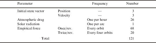
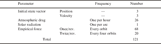
The estimated parameters and strategies used in this study (called the “reference case”) are summarized in Table 2. It should be noted that only 121 parameters are estimated for one full day orbit since there are no ambiguity parameters; a significant computation load reduction, as compared to 13200 ambiguity parameters (from about 100 IGS ground stations) in the double-differenced dynamic POD (Švehla and Rothacher, Reference Švehla and Rothacher2003). The processing time to estimate the 121 parameters for the 26-hour arc is about 2·5 hours (30 minutes per iteration) on a 3 GHz PC platform.

Table 2.

The estimated parameters for the “reference case.”

6. ANALYSIS OF THE ORBIT SOLUTION

In most research on satellite orbits, the results are validated by their comparison to an independent method, such as Satellite Laser Ranging (SLR) or altimeter crossover data; or by an internal check for the overlapping arcs, in the absence of the absolute reference orbit. Since the RSO is assumed to be the best orbit available, the triple difference-based CHAMP orbits are compared to the RSO in this study. As a first step of the comparison, the consistency test between two orbit solutions was performed. This can be done by testing the sum of the residuals with the given stochastic constraints of the published RSO. Let the Gauss-Markov Model with stochastic constraints be given by

(12)

(13)

where n denotes the number of observations, m the number of unknown parameters and l denotes the number of stochastic constraints. In order to check the stochastic constraints to be consistent with the observation model, it is necessary to test the null hypothesis of

(14)

with the alternative hypothesis of

(15)

The test statistics for the hypothesis testing can be represented by

(16)

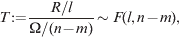
where Ω represents the sum of squared residuals from the original model, and R denotes the change of the sum of squared residuals due to the stochastic constraints. As can be seen in Equation (16), the test statistics follow the F-distribution with the degree of freedom of l and n−m. Let α be the significance level of the test. Then, the null hypothesis, H _o, is rejected if T>F _α(l, n−m).

Table 3 shows the results of the test statistics with the significance level of 5%. The total of 3110 epochs of CHAMP orbit is constrained with the accuracy given in the table, while the total number of 139,225 observations is used in the adjustment. From this table, it can be concluded that these two orbits are consistent as long as the accuracy of the published RSO is not better than 4 cm. Thus, despite different models used in both solutions, the final results are statistically consistent. Thus, any further improvement in the orbital solution can be only achieved with the new information, i.e., another type of measurement would be required.

Table 3.

The test statistics for consistency test.

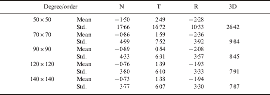
Table 4 shows the resulting orbit solution for different degree and order of the geopotential model used. The geopotential model used in this study, EIGEN2, has a maximum degree/order of 140. As can be expected, considering CHAMP's altitude, the CHAMP orbit is visibly sensitive to the degree/order up to 70 and only moderate, but increasing, improvement can be obtained for the higher degree/order.

Table 4.

Orbit errors for different degree/order of the gravity models w.r.t. the RSO in the RTN frame (unit: cm).

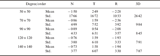
One thing to be noted here is that the error in the along-track direction is almost two times that of the other two components, especially in the case of the solutions with the degree/order 120 and 140. This comes from the fact that the most dominant nonconservative force, atmospheric drag, is in the opposite direction of the along-track component. In reality, the along-track component diverges the fastest if the atmospheric drag is not modelled appropriately.

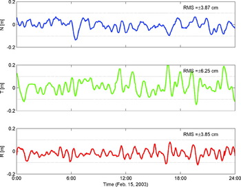
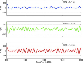
Figure 2 illustrates the orbit solution in the RTN frame for the “reference case,” i.e., the case of the geopotential degree/order 120 and 1 hour interval for the atmospheric drag parameter estimation. The orbit error is plotted for the 24-hour span, although it converged for the entire 26 hours of arc. Another orbit accuracy assessment can be obtained by the internal consistency check of the overlapping arcs. Figure 3 shows the 24-hour orbit difference between the “reference case” and the 30-hour arc, which extends 3 hours before and after one full day. As can be seen in the figure, the two orbit solutions are close to each other, except for the first few epochs; the results show the difference of less than 1·3 cm of RMS in each direction and 2 cm in 3D RMS (not shown in this figure). The difference at the beginning of the arc is due to the fact that the coordinates at the first epoch were unknown in the “reference case,” and no epochs were estimated before the first epoch.

Figure 2.

Orbit errors for the “reference case” w.r.t. the RSO in the RTN frame.

Figure 3.

Internal consistency of the orbit solution; the “reference case” vs. 30 hours of arc.

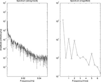
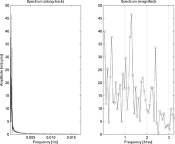
As discussed earlier, the force modelling of the satellite dynamics is not accurate enough for the precise orbit determination. Therefore, the empirical force parameters can be included in the state vector to improve the orbit solution. A closer look at the STAR accelerometer data reveals the periodic properties of the once- and twice-per-revolution nonconservative forces (Figure 4a), which are predominantly in the along-track component. Figure 4b shows the orbit solution of the “reference case” after these empirical parameters are modeled in the dynamic POD, that is, once- and twice-per-revolution components are significantly reduced in the Fourier spectrum of the orbit error in the along-track direction. One thing that should be mentioned here is that the along-track and radial components are estimated for the twice-per-revolution empirical forces, which gives better results than the other case (i.e., estimating the cross- and along-track components). This is not clearly understood and should be investigated further.

Figure 4a.

Fourier spectrum of STAR accelerometer data for CHAMP (along-track).

Figure 4b.

Fourier spectrum of the orbit error (along-track).

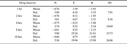
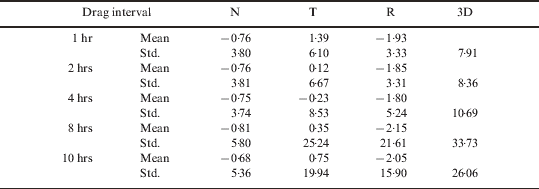
In order to find out the optimal arc length of the atmospheric drag force parameters, a total of five different cases were tested based on the “reference case” (Table 5); the atmospheric drag parameters are estimated every 1 hr, 2 hrs, 4 hrs, 8 hrs and 10 hrs of arc, where 1 hr arc case corresponds to the “reference case.” The results suggest that the orbit errors will dramatically increase if the drag coefficient is estimated with the frequency less than once every 4 hours. This is because the atmospheric density at CHAMP altitude can fluctuate rapidly due to the varying density of the Sun flux particles and changing geographic location of the CHAMP satellite.

Table 5.

The statistics of orbit relative to the “reference case” with various time interval for the atmospheric drag parameter estimation.

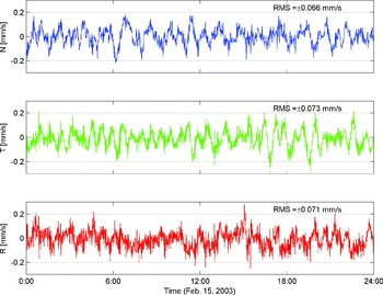
The velocity of the CHAMP satellite is obtained simultaneously by solving the equations of motion of the satellite in the dynamic POD through the numerical integration techniques. Figure 5 shows the velocity errors in each component of the CHAMP satellite. The velocity errors are computed by differencing the estimated satellite velocity with the published RSO velocity which is then transformed to the inertial frame. One thing to be noted here is that the noise level of the three components is almost the same, although the along-track component is still a little higher than the other two. The resulting velocity errors are at the level of 0·07 mm/s in each component and 0·12 mm/s in 3D RMS. These RMS of fit results are comparable or even better than the precision of fit of the CHAMP dynamic velocity estimates among the POD analysis centres, which were computed by cross-comparison among the solutions and reported at below 0·1 mm/s level (Švehla and Rothacher, Reference Švehla and Rothacher2003).

Figure 5.

Velocity errors in the RTN frame for the “reference case” w.r.t. RSO.

7. SUMMARY AND CONCLUSIONS

The dynamic orbit determination for LEO satellite using the triple differencing technique was demonstrated using the CHAMP satellite data. This technique makes it possible to implement a simple, efficient and accurate algorithm in the near real-time mode. The modelling of the atmospheric drag force is crucial in the dynamic orbit determination, because it accounts for most of the nonconservative forces. The proper modelling of the atmospheric drag, including the optimal arc length for the drag parameter estimation, provides an orbit solution of about 8 cm in 3D RMS of fit with respect to RSO. The hypothesis test shows that the dynamic orbit solution obtained in this study is statistically consistent with the published RSO when it is not better than 4 cm in terms of an absolute accuracy. The orbit errors, as a function of the degree/order of the geopotential model used, were also analyzed here. As expected, the higher the degree of the geopotential model, the better the results obtained; however, more sensitivity was observed for degree/order up to 70. Therefore, one should consider expanding the degree and order up to 200 or more, using the newly published EIGEN-CG01C model (CHAMP, 2005). The different gravity models were not tested thoroughly in this study because the EIGEN2 gravity model is generated using CHAMP data only, and is thus assumed to be the best for CHAMP dynamic orbit determination.

The internal consistency check shows that the redundant part before the main arc does not play an important role in the final orbit solution. That is, the orbit solution from 26 hours of arc is comparable to that from the 30-hour arc. Also, the orbit solution converges very quickly if the scaling factors for the atmospheric drag and the empirical force parameters are estimated at intervals equal to or shorter than 2 hours. Therefore, from the computational efficiency point of view, it is highly beneficial to estimate the initial state vector at the beginning of the target arc.

The estimated orbit solution with once- and twice-per-revolution empirical forces significantly reduced the orbit errors at both frequencies. However, the actual correlation between the along-track and the radial components for the twice-per-revolution parameters is not clearly verified; this should be studied more rigorously in the future studies. The time interval for the estimation of the atmospheric drag parameters should not exceed 2 hours in order to obtain a precise orbit solution, because of the rapid change in the atmospheric density along the trajectory. The CHAMP velocity results prove to fit the reference RSO solution with RMS better than 0·073 mm/s in each component, which is comparable to the CHAMP dynamic velocity from any other analysis centres.