
 rz





1. Introduction
Magnetised plasmas are central to a wide range of applications, including magnetic-confinement fusion, plasma-assisted materials processing and electric propulsion. In magnetic mirror and magnetic-nozzle configurations, converging–diverging magnetic fields guide plasma flow along the field while providing cross-field confinement (Budker Reference Budker1959; Post Reference Post1987; Díaz Reference Díaz2001; Charles Reference Charles2009; Takahashi Reference Takahashi2019; Wu et al. Reference Wu, Chen, Ren, Wang, Zhang, Wang and Tang2025). The resulting dynamics couples axial confinement and acceleration, sheath formation at material boundaries, trapped particle populations and cross-field transport, and is intrinsically kinetic and nonlinear. In particular, open-field systems naturally develop non-Maxwellian distributions and strong spatial gradients, so reduced fluid closures can miss key mechanisms controlling confinement and losses.
A large body of magnetic mirror analytic theory relies on reduced-kinetic descriptions that exploit strong plasma magnetisation and the near-axis approximations for the flow (Pastukhov Reference Pastukhov1974; Post Reference Post1987). Reduced-kinetic modelling of the mirror expander and related flow regimes has also been pursued in modern theory and simulation studies (Wetherton et al. Reference Wetherton, Le, Egedal, Forest, Daughton, Stanier and Boldyrev2021; Jimenez et al. Reference Jimenez, Smolyakov, Chapurin and Yushmanov2022; Francisquez et al. Reference Francisquez, Rosen, Mandell, Hakim, Forest and Hammett2023; Dorf et al. Reference Dorf, Dorr, Geyko, Ghosh, Umansky and Angus2025; Tyushev et al. Reference Tyushev, Smolyakov, Sabo, Groenewald, Necas and Yushmanov2025). Such approaches are valuable for isolating axial physics and for scanning parameters efficiently, but they cannot represent several effects that become important once finite gyroradius and azimuthal degrees of freedom are allowed. Two examples are (i) radial charge separation driven by finite-ion-Larmor-radius (FLR) and polarisation dynamics when the ratio of the ion gyroradius
 $\rho_i$
to the radial density-gradient scale
 $L_n$
becomes large,
 $\rho _i/L_n \sim 1$
, and (ii) the emergence of azimuthal structures that can self-consistently organise
 $\boldsymbol{E} \times \boldsymbol{B}$
flows (where
 $\boldsymbol{E}$
and
 $\boldsymbol{B}$
denote the electric and magnetic fields, respectively), generate non-ambipolar radial currents, and modify both confinement and axial acceleration. Quantifying these multidimensional effects and associated transport is essential for the interpretation of the reduced-model predictions and for assessing performance limits in real device-scale configurations.
Device-scale multidimensional simulations of mirror plasmas remain comparatively scarce, and many existing efforts employ hybrid formulations (e.g. kinetic ions with fluid electrons) tailored to specific operating regimes (Lindvall et al. Reference Lindvall, Holmberg, Bendtz, Scheffel and Lundberg2025; Tran et al. Reference Tran2025). Fully kinetic simulations (kinetic ions and electrons) in realistic geometries are substantially more demanding, yet they are uniquely positioned to capture self-consistent charge separation, sheath dynamics and instability-driven transport without imposing ad hoc closures. In this work, we use fully kinetic particle-in-cell (PIC) simulations to bridge an axisymmetric two-dimensional
 $(r,z)$
(2-D-
 $rz$
) model and a fully three-dimensional (3-D) Cartesian
 $(x,y,z)$
model within the same numerical framework. This allows direct, controlled comparisons between reduced and full geometries under closely matched boundary conditions and injection parameters, and enables direct comparison with our earlier 1-D drift-kinetic PIC study of the same configuration (Tyushev et al. Reference Tyushev, Smolyakov, Sabo, Groenewald, Necas and Yushmanov2025), which is based on the drift-kinetic approximation using the electrostatic direct implicit particle-in-cell (EDIPIC) framework (Sydorenko Reference Sydorenko2006). Multidimensional 2-D-
 $rz$
and 3-D simulations are performed within the WarpX framework (Fedeli et al. Reference Fedeli2022; Vay et al. Reference Vay2025).
The goals of this paper are threefold. First, in the axisymmetric limit, we test the robustness of axial confinement and acceleration demonstrated earlier in 1-D models as radial charge separation in the 2-D-
 $rz$
model becomes noticeable, and we quantify how a non-uniform radial potential modifies near-axis profiles and wall losses. Second, allowing a full 3-D evolution, we track the onset and saturation of azimuthal structures, and relate their mode number content and amplitude to radial plasma spreading and enhanced radial losses. We pay particular attention to how the finite ion temperature and associated FLR effects reshape the instability spectrum and the resulting transport. Third, we examine the effects of the
 $E \times B$
shear on azimuthal fluctuations and on cross-field losses by applying the bias as a boundary condition at the endplate. Although our simulations are primarily motivated by open-mirror fusion applications (Gota et al. Reference Gota, Binderbauer, Tajima, Smirnov, Putvinski and team2021; Endrizzi et al. Reference Endrizzi2023), our methodology and results are also of interest for electric propulsion applications (Díaz Reference Díaz2001; Charles Reference Charles2009; Takahashi Reference Takahashi2019; Wu et al. Reference Wu, Chen, Ren, Wang, Zhang, Wang and Tang2025), in particular, by complementing 2-D PIC simulations of the magnetic nozzle (Hu et al. Reference Hu, Huang, Cao and Sun2021; Andrews, Di Fede & Magarotto Reference Andrews, Di Fede and Magarotto2022; Chen et al. Reference Chen, Wang, Tang, Ren, Li, Zhang, Cao and Cao2022) and extending them to a full 3-D geometry.
In addition, we employ a semi-implicit, energy-conserving electrostatic PIC integrator (Barnes & Chacón Reference Barnes and Chacón2021; Groenewald et al. Reference Groenewald, Barnes, Tyushev, Zhang, Huebl, Necas, Smolyakov, Vay, Tajima and Dettrick2024; Hedlof et al. Reference Hedlof, Barnes, Groenewald, Necas, Smith, Lau, Brandt, Zhang, Eckert and Hooper2026) that introduces controlled numerical permittivity (equivalently, an enlarged effective Debye length), enabling stable high-density simulations and exploring azimuthal modes in such regimes of practical interest.
The core methodology and a substantial portion of the results in this manuscript were developed as part of a PhD thesis by Tiushev (Reference Tiushev2025).
The paper is organised as follows. Section 2 describes the simulation model, magnetic field, boundary conditions and numerical parameters. Section 3 presents axisymmetric (2-D-
 $rz$
) results, emphasising radial confinement, charge separation and the impact on axial acceleration. Section 4 analyses the full 3-D regime, including azimuthal mode structure, radial spreading and associated radial losses, with a focus on the dependence on ion temperature. Section 5 investigates the effects of applied bias and the resulting shear stabilisation. Section 6 introduces the semi-implicit, energy-conserving PIC formulation used to access high-density regimes. Section 7 summarises the main findings and their implications for modelling of transport and its control in open magnetic mirror configurations.
2. The simulation model and boundary conditions
In this study, we employ the WarpX code (Fedeli et al. Reference Fedeli2022; Vay et al. Reference Vay2025), a modern PIC code that supports both cylindrical
 $(rz)$
and fully 3-D
 $(x,y,z)$
geometries within the same implementation. This makes it particularly well suited for our purposes, as it allows us to cross-check results between reduced and full models under similar boundary conditions. The simulations were performed using the public WarpX version 25.09. Unless stated otherwise, we retained the default WarpX algorithms for this version. In particular, the electrostatic simulations use the standard energy-conserving field-gathering scheme, default mesh filtering and first-order particle shape factors. The semi-implicit cases use the same general WarpX PIC framework, with the additional modification to the Poisson equation described in § 2.4.
WarpX is also optimised for GPU acceleration, which is essential for handling the large number of particles and fine spatial resolution required in this study. The
 $(rz)$
simulations were performed on NVIDIA V100 GPUs (Mist server, Digital Research Alliance of Canada), while the more demanding 3-D runs were performed on two NVIDIA A100 GPUs (Narval server, Digital Research Alliance of Canada).
These simulations use a
 $0.5\,\mathrm{m}$
-long mirror (
 $0.25\,\mathrm{m}$
confinement region plus
 $0.25\,\mathrm{m}$
expander region), with
 $B$
rising from
 $0.05$
to
 $0.5\,\mathrm{T}$
in the confinement region and falling from
 $0.5$
to
 $0.01\,\mathrm{T}$
in the expander. The plasma consists of electrons and singly ionised hydrogen ions,
 $H^+$
, with ion charge
 $q_i=+e$
, where
 $e$
is the elementary charge, and the physical ion-to-electron mass ratio
 $m_i/m_e\approx 1836$
. The computational cost depends on the complexity of the different regimes. For the low ion-temperature case (
 $T_i=30$
eV), the instability develops slowly, reaching a quasi-steady state only after
 ${\sim} 60\,\unicode{x03BC}$
s, so the 3-D simulation required nearly three months of real time to complete, while the corresponding
 $rz$
run took only several days. For the high ion-temperature case (
 $T_i=600$
eV), the instability develops much faster, within approximately
 $10\,\unicode{x03BC}$
s, and the 3-D simulations typically required about two weeks of real time, while the
 $rz$
simulations again finished within several days.
Magnetic-field streamlines with colour bar representing the
 $B_z$
component of the magnetic field.

2.1. Magnetic field
Our simulation models are designed to enable direct comparison between axisymmetric (2-D-
 $rz$
) and fully 3-D cases, and to remain as close as possible to the magnetic-field profiles used in our earlier 1-D study (Tyushev et al. Reference Tyushev, Smolyakov, Sabo, Groenewald, Necas and Yushmanov2025). In the multidimensional geometry, however, we impose a zero normal electric field (
 $E_n=0$
) at the source boundary as a symmetry-motivated electrostatic boundary condition, where the magnetic field is expected to be normal to the injection plane. Therefore, to reduce the field curvature in the injection plane, we introduce a shaping coefficient
 $\kappa$
in (2.1) that flattens the axial variation of
 $B$
near the source plane.
The magnetic field is prescribed by the poloidal flux function, equivalent to the paraxial representation for a generic converging–diverging magnetic mirror
 \begin{align} \psi (r,z) = \frac {1}{2} B_0 r^2 \begin{cases} \displaystyle \frac {1 + (\kappa - 1)\left (z/z_0\right )^2}{1 + (R \kappa - 1)\left (z/z_0\right )^2}, & z \lt 0, \\[1.0ex] \displaystyle \frac {1}{1 + (K - 1)\left (z/z_0\right )^2}, & z \gt 0, \end{cases} \end{align}
where
 $z\in [-z_0,z_0]$
, with
 $z_0=0.25\,\mathrm{m}$
the system half-length, and where
 $B_0=0.5\,\mathrm{T}$
is the axial magnetic field in the mirror throat (
 $z=0$
),
 $R=B_0/B(-z_0)$
is the confinement-side mirror ratio, and
 $K = B_0 / B(z_0)$
the expander-side expansion ratio. With
 $\hat{\boldsymbol{e}}_\theta$
denoting the azimuthal unit vector, the magnetic field is obtained from the poloidal flux function
 $\psi$
as
 \begin{align} \boldsymbol{B}=\frac {1}{r}\,\boldsymbol{\nabla }\psi \times \hat {\boldsymbol{e}}_\theta ,\qquad B_\theta =0 . \end{align}
The resulting field is shown in figure 1, where arrows indicate the field direction and the colour scale represents the axial component
 $B_z(r,z)$
. Unless stated otherwise, the multidimensional simulations use the modified profile with
 $\kappa =5$
in (2.1); the case
 $\kappa =1$
is retained as the 1-D-consistent reference.
2.2. Boundary conditions
The boundary conditions in the axisymmetric (2-D-
 $rz$
) and fully 3-D simulations are identical. For clarity, we illustrate them in the
 $rz$
geometry. Figure 2 shows the computational domain and boundary conditions.
A schematic diagram of the set-up of simulations (3-D and 2-D-
 $rz$
cases) for a magnetic mirror.

2.2.1. The left boundary
The boundary (blue rectangle in figure 2 at
 $z_0=-0.25\,\mathrm{m}$
) represents the injection wall, which is a boundary between the plasma (generation) source and the converging–diverging mirror. The plasma source (not modelled in our approach) is represented as a Maxwellian thermal reservoir with prescribed electron and ion temperatures, providing an idealised model of source conditions similar to those of the gas dynamic trap. While the boundary is not a symmetry plane, we still retain
 $E_n=0$
as a boundary condition.
Electrons and ions are injected at equal particle rates, so that the system is globally ambipolar. Injected particles are sampled from a flux Maxwellian distribution for the velocity component in
 $z$
and a regular Maxwellian distribution for
 $x$
and
 $y$
. The electron injection temperature is fixed at
 $T_0^e=300\,\mathrm{eV}$
, while ions are injected with either
 $T_0^i=600\,\mathrm{eV}$
or
 $30\,\mathrm{eV}$
, depending on the case.
The injection rate is non-uniform in radius and follows a Gaussian profile centred at
 $r=0$
with a radial standard deviation
 $\sigma =7\,\mathrm{cm}$
(purple curve in figure 2), representing a radially localised plasma source. The value of
 $\sigma$
is chosen to be comparable to the ion Larmor radius in the source magnetic field for the
 $T_0^i=600\,\mathrm{eV}$
case and is kept fixed across all simulations.
Since our simulations are collisionless, particles outside the loss cone remain trapped indefinitely; we therefore re-mix particles that return to the source plane. Purely specular reflection would preserve their energy and pitch angle but would not replenish the energetic and loss-cone populations removed by axial losses. Since the model contains no volumetric heating mechanism, the confined distribution would progressively cool and depart from the prescribed thermal-source regime. Particles returning to this wall are therefore re-emitted at the original injection temperature using a Maxwell-type mixed reflection model: a fraction is diffusely re-emitted from the same Maxwellian velocity distribution, while the remainder is specularly reflected. The thermalisation probability follows the same Gaussian radial profile as the injected source, being unity on the axis and decreasing with radius. This choice maintains the prescribed source temperatures and radial profile while avoiding large near-wall conductivity at large radii.
As noted above, the symmetry-motivated electrostatic boundary condition
 $E_n=0$
is not fully consistent with the finite particle flux through the
 $z=-0.25$
m plane, which represents the interface between the mirror and the plasma source. Consequently, the particle boundary condition does not impose
 $v_{\parallel i}=v_{\parallel e}=0$
, where
 $v_{\parallel i}$
and
 $v_{\parallel e}$
are the parallel ion and electron flow velocities, respectively. Instead, finite incoming and outgoing particle fluxes are present at the source boundary. In our previous 1-D study (Tyushev et al. Reference Tyushev, Smolyakov, Sabo, Groenewald, Necas and Yushmanov2025), we showed that the time-averaged plasma profiles remained well behaved for two different sets of boundary conditions, although the
 $E_n=0$
condition produced high-frequency numerical fluctuations. No similar fluctuations were observed in the present multidimensional simulations. Retaining the
 $E_n=0$
condition enables direct comparison between the previous 1-D results and the present 2-D and 3-D simulations. More realistic plasma-source models will be considered in future work.
2.2.2. Radial wall (
 $r=0.4\,\mathrm{m}$
) and right boundary (
$z=0.25\,\mathrm{m}$
)


The radial wall and the right boundary (green rectangles) absorb both species and are held at fixed potential,
 $\phi =0$
. In a biased variant, the endplate (right boundary) potential is prescribed as a linear function of the radius, ranging from
 $-3000$
V at
 $r=0$
to
 $0$
V at the radial wall.
2.3. Simulation parameters
Simulation parameters and initialisation are as follows. Starting from a vacuum with a fixed injection flux produces long transients before a quasi-steady state is obtained, which is prohibitive in multidimensional runs. To accelerate initialisation, the particle injection flux at the left boundary is adjusted in time using a proportional–integral–derivative controller to reach and maintain a prescribed density on the axis
 $n(0)=10^{16}\,\mathrm{m^{-3}}$
(for
 $z\lt 0$
). In the 2-D-
 $rz$
geometry, this procedure reaches a quasi-steady state within
 ${\sim} 10\,\unicode{x03BC} \mathrm{s}$
, whereas in three dimensions the subsequent evolution proceeds on the characteristic instability growth and saturation time scale. The values of the steady-state injection flux are reported below for each case.
The computational domain spans
 $0.8 \times 0.8 \times 0.5\,\mathrm{m}$
and is resolved with a
 $256 \times 256 \times 128$
mesh in three dimensions and
 $128 \times 128$
in the 2-D-
 $rz$
geometry. For the target density
 $n=10^{16}\,\mathrm{m}^{-3}$
, the minimum ratio of Debye length
 $\lambda_D$
to cell size
 $\Delta x$
is
 $\lambda _D/\Delta x \approx 0.3$
, so the Debye length is under-resolved. In explicit momentum-conserving PIC schemes, such under-resolution can lead to numerical heating; here, we use an energy-conserving scheme, which has been shown to remain accurate for
 $\lambda _D/\Delta x$
as low as
 ${\sim} 0.1$
in the relevant regimes (Powis & Kaganovich Reference Powis and Kaganovich2024). Under-resolution of
 $\lambda _D$
smooths fine-scale charge-separation layers; however, in our set-up, the smallest
 $\lambda _D/\Delta x$
occurs only near the axis in the region of the converging magnetic field, and auxiliary 1-D implicit simulations (Tyushev et al. Reference Tyushev, Smolyakov, Sabo, Groenewald, Necas and Yushmanov2025) indicate no measurable impact on macroscopic plasma parameters.
The time step is chosen as
 $dt = 5 \times 10^{-12}$
s, corresponding to
 $0.4 \,\omega _{ce}^{-1}$
at the maximum magnetic field (
 $B=0.5$
T), where
 $\omega_{ce}$
is the electron cyclotron frequency. A stricter condition (Birdsall & Langdon Reference Birdsall and Langdon1985) would require
 $dt \lt 0.2 \,\omega _{ce}^{-1}$
, but since the region of maximum field is small, we do not expect a significant effect on electron rotation. For reference, the electron plasma frequency
 $\omega_p$
gives
 $0.2\,\omega _p^{-1} \approx 3.5 \times 10^{-11}$
s. With the chosen grid spacing and time step, the Courant–Friedrichs–Lewy number is
 $\mathrm{CFL}\approx 0.02$
.
The magnetic mirror ratios are
 $R=10$
on the source side (
 $z \in [-0.25,0]$
) and
 $K=50$
on the expander side (
 $z \in [0,0.25]$
). Each macroparticle represents
 $5\times 10^6$
physical particles in the
 $rz$
simulations. Because the plasma density varies strongly across the system, the single average number of particles per cell is not very informative: in the converging part, we observe approximately
 $2200$
particles per cell, while in the expander, this decreases to approximately
 $50$
. The total number of macroparticles in the system is approximately
 $1.35 \times 10^8$
per species.
In three dimensions, each macroparticle corresponds to
 $5\times 10^5$
physical particles, giving a total of order
 $2.5\times 10^8$
macroparticles per species (the exact value varies from case to case). On average, in the source region we have approximately
 $100$
particles per cell, while in the expander regions this value is approximately
 $10$
.
2.4. Semi-implicit scheme for high-density simulations
In addition to explicit baseline runs, we have performed modelling with plasma densities of the order of
 $n=10^{18}\,\mathrm{m^{-3}}$
, two orders of magnitude above the nominal
 $10^{16}\,\mathrm{m^{-3}}$
. At fixed electron temperature, the Debye length scales as
 $\lambda _D\propto \sqrt {T_e/n}$
, so increasing
 $n$
by a factor of
 $100$
reduces
 $\lambda _D$
by a factor of
 $10$
. A fully explicit PIC treatment that resolves both
 $\lambda _D$
and
 $\omega _{pe}$
would therefore require
 $\Delta x$
to decrease by
 ${\sim} 10$
in each direction, i.e. a
 ${\sim} 10^3$
increase in the number of cells in three dimensions. Maintaining adequate particles per cell would then increase the total particle count to
 $\mathcal{O}(10^{11}$
–
 $10^{12})$
, which is beyond the available GPU memory and makes fully explicit simulations at
 $n=10^{18}\,\mathrm{m^{-3}}$
impractical.
To access such a high-density regime, we use the semi-implicit electrostatic PIC (SIPIC) formulation implemented in WarpX (Groenewald et al. Reference Groenewald, Barnes, Tyushev, Zhang, Huebl, Necas, Smolyakov, Vay, Tajima and Dettrick2024). The SIPIC formulation treats the fast electron response implicitly by solving a modified Poisson equation that includes an electron-polarisation contribution proportional to the local electron density. This reduces the effective electron plasma-frequency constraint on the time step while retaining the low-frequency dynamics relevant to transport. The resulting operator is not equivalent to multiplying
 $\varepsilon _0$
by a constant: the additional term varies in space and time and is implemented in an energy-conserving manner. Schematically, the modified operator can be written in terms of an effective permittivity
 \begin{align} \varepsilon _{\mathrm{eff}}=\varepsilon _0\!\left [1+C_{\mathrm{SI}}\Big (\tfrac {\omega _{pe}\,\Delta t}{2}\Big )^{2}\right ], \end{align}
with
 $C_{\mathrm{SI}}=4000$
in the present simulations, which yields
 $\varepsilon _{\mathrm{eff}}\approx 100\,\varepsilon _0$
in the highest-density regions. Since the corresponding effective Debye length scales as
 $\lambda _D^{\mathrm{eff}}\propto \sqrt {\varepsilon _{\mathrm{eff}}}$
, this increases
 $\lambda _D^{\mathrm{eff}}$
by approximately one order of magnitude, allowing the same mesh spacing and time step as in explicit cases.
Unlike a spatial spectral filter, this modification does not directly select particular Fourier components and therefore does not introduce a characteristic damping wavelength. Defining
 $\kappa =\varepsilon _{\mathrm{eff}}/\varepsilon _0$
, the corresponding effective plasma frequencies are reduced according to
 $\omega _{ps}^{\mathrm{eff}}=\omega _{ps}/\sqrt {\kappa }$
(Hedlof et al. Reference Hedlof, Barnes, Groenewald, Necas, Smith, Lau, Brandt, Zhang, Eckert and Hooper2026). For
 $\kappa \simeq 100$
in the highest-density regions, the effective plasma frequencies are therefore reduced by approximately a factor of ten. The effective Debye length introduced above represents an electrostatic screening scale rather than a sharp wavelength cutoff; the influence of the semi-implicit operator on a particular mode depends on its full dispersion relation and on whether the relevant spatial and temporal scales are resolved.
2.5. One-dimensional reference model
For comparison, we also consider a 1-D drift-kinetic reference model based on EDIPIC (Tyushev et al. Reference Tyushev, Smolyakov, Sabo, Groenewald, Necas and Yushmanov2025). The 1-D domain has the same axial length
 $2z_0=0.5\,\mathrm{m}$
and uses the same injection temperatures (
 $T_0^e=300\,\mathrm{eV}$
and
 $T_0^i =600\,\mathrm{eV}$
) as multidimensional simulations. The 1-D model differs from the 2-D/3-D set-up in four elements: (i) radial structure is not resolved (all quantities are uniform in radius); (ii) the magnetic field is prescribed by the 1-D axial profile corresponding to
 $\kappa =1$
in (2.1) instead of
 $\kappa =5$
; (iii) the electrostatic boundary conditions are
 $\phi =0$
at the injection wall and a floating boundary at the right endplate (the endplate potential adjusts so that the net current to the wall vanishes in steady state); and (iv) drift-kinetic equations are used for electrons and ions, and a modified Poisson equation (for inhomogeneous magnetic field) is solved using the EDIPIC framework. The injection current density
I
inj
is chosen to match the target on-axis density used in the multidimensional cases
 $n(0)=10^{16}\,\mathrm{m^{-3}}$
; for the reference case this corresponds to
 $I_{\mathrm{inj}}=22\,\mathrm{A\,m^{-2}}$
.
3. Radial plasma confinement and axial acceleration in 2-D-
$rz$
geometry

In this section, we study the plasma behaviour in the 2-D-
 $rz$
configuration, focusing on the high ion-temperature regime with
 $T_i=600$
eV. We consider this case because, at
 $T_i=30$
eV, finite-ion-orbit effects are weak, losses to the radial wall in the converging region of the mirror are negligible and the 1-D and 2-D-
 $rz$
results are identical. In contrast, finite-ion-orbit effects become important at
 $T_i=600$
eV. Figure 3 shows the emergence of a distinct ‘bump’ in the electrostatic potential, reaching values of order
 $10\,T_0^e$
. After multiple bounces between the injection boundary and the magnetic throat, ions rethermalise at the injection boundary, so their velocity and radial position change, producing radial transport. Consequently, some ions are lost to the side wall, while others acquire sufficient parallel velocity to escape axially through the mirror.
A quantitative estimate shows relatively low losses: approximately 5 % of the injected flux escapes radially at
 $T_i=600$
eV. The losses are predominantly in the ion component, making them locally non-ambipolar. The formation of a self-consistent potential structure at the edge, mitigating the radial ion expansion in the converging part of the mirror, is an important feature of the 2-D-
 $rz$
model. The radial scale of this structure can be understood qualitatively from the FLR redistribution. Although the plasma is injected with a Gaussian radial profile, ions with
 $\rho _i\simeq 7$
cm sample a broader radial region than the strongly magnetised electrons. This produces an electron-rich region at smaller radii and an ion-rich region at larger radii, generating an electric field that tends to restore the radial balance. Farther outward, the ion space charge becomes dominant and the radial electric field reverses, producing the potential maximum. This picture is complicated by electron redistribution associated with thermalisation at the source boundary, which compensates the initial charge separation in the central region. As shown in the middle panel of figure 3, the potential profiles along the field lines launched at
 $r=0$
(orange curve) and
 $r=10$
cm (green curve) nearly coincide throughout the converging part of the mirror, indicating that the potential remains nearly radially flat over the central region up to
 $r\simeq 10$
cm. This radial scale is of the order of the source width,
 $\sigma =7$
cm. Beyond this central region, the electric field reaches zero after an additional radial distance of the order of
 $2\sigma$
, placing the potential maximum at
 $r\simeq 20$
–
 $25$
cm. The amplitude and precise location of the potential maximum are determined self-consistently by the radial charge balance, radial losses and the boundary conditions and therefore cannot be estimated from the ion Larmor radius alone.
We note that the formation of a radial confining potential due to the difference between the ion and electron orbit radii was reported by Shoucri et al. (Reference Shoucri, Pohn, Knorr, Bertrand, Kamelander, Manfredi and Ghizzo2000) in Vlasov simulations and later by Lee & White (Reference Lee and White2017), together with some experimental observations in a tokamak; see also Shoucri (Reference Shoucri2018) for further discussion and references. Non-monotonic potential structures at the edge of a plasma jet also appear to have been observed in magnetic-nozzle experiments by Little & Choueiri (Reference Little and Choueiri2016) and in PIC simulations by Chen et al. (Reference Chen, Wang, Tang, Ren, Li, Zhang, Cao and Cao2020, Reference Chen, Wang, Ren, Tang, Wu and Li2022).
Electron and ion densities and potential for the 2-D-
 $rz$
model at
 $T_i = 600$
eV.

A direct comparison between the 1-D and 2-D-
 $rz$
results for the
 $T_i = 600$
eV case is shown in figure 4. The axial density profiles (top panel of figure 4) are broadly similar. The middle panel illustrates the electrostatic potential, where the total drop in one dimension is larger than in the 2-D-
 $rz$
case. This difference is associated with enhanced radial ion losses. Since the net current through all boundaries is constrained to zero, the outward radial ion current into the wall is closed by the electron current flowing along the field lines. Several profiles are also plotted along field lines launched at various radii, which remain relatively unchanged up to
 $r \simeq 0.1$
m, where the bulk of the plasma is located.
Plasma density (top), electrostatic potential (middle) and ion velocity (bottom) along magnetic-field lines for the 1-D and 2-D-
 $rz$
models at
 $T_i = 600$
eV, shown as functions of the axial coordinate
 $z$
. The initial radial position of each field line is indicated in the legend at
 $z=-0.25$
m (injection plane at the left wall). For the 2-D-
 $rz$
model, the top graph is plotted for
 $r=0$
.

Figure 4. Long description
Three line graphs depict plasma density, electrostatic potential, and ion velocity along magnetic-field lines for 1-D and 2-D models. Panel A: The top graph shows plasma density (n, m^-3) as a function of the axial coordinate (z, m). The blue solid line represents electron density in the 2-D model, the blue dashed line represents electron density in the 1-D model, the red solid line represents ion density in the 2-D model, and the red dashed line represents ion density in the 1-D model. Panel B: The middle graph shows the electrostatic potential (eφ/T_e) as a function of the axial coordinate (z, m). The blue line represents the 1-D model, the orange line represents the 2-D model at r = 0 cm, the green line represents the 2-D model at r = 10 cm, and the red line represents the 2-D model at r = 15 cm. Panel C: The bottom graph shows ion velocity (v_i∥/c_s) as a function of the axial coordinate (z, m). The blue line represents the 1-D model, the orange line represents the 2-D model at r = 0 cm, the green line represents the 2-D model at r = 10 cm, and the red line represents the 2-D model at r = 15 cm.
The bottom panel of figure 4 shows the comparison of the velocity in 1-D (described in § 2.5) and
 $rz$
simulations. The 1-D profile coincides closely with the
 $rz$
curve at
 $r = 0.1$
m, but the onset of acceleration occurs earlier in the 1-D case. This offset originates from the different field profiles: the 1-D simulations use the unmodified magnetic potential, (2.1) with
 $\kappa = 1$
, while the
 $rz$
model employs the modified form with
 $\kappa = 5$
, designed to produce nearly perpendicular field lines near the left wall. Despite these differences, both models converge to the same velocity at
 $z=0$
and follow each other in the expansion region.
The curve
 $r=0$
(orange) in the bottom panel of figure 4 illustrates a well-known artefact of cylindrical PIC geometry: enhanced noise and oscillations near the axis,
 $r\rightarrow 0$
, due to the collapsing cell volume
 $V\sim 2\pi r\,\Delta r\,\Delta z$
, where (
 $\Delta r$
) is the radial cell size. At moderate ion temperature, this issue can be mitigated by increasing the number of particles near
 $r=0$
, but at high
 $T_i$
the large-ion-orbit width exacerbates the problem. Ion gyromotion then advances a particle by an azimuthal arc that can exceed the local geometric scale
 $r$
, i.e.
 $v^i_\perp \Delta t/r \gt 1$
. This geometric CFL overstep near
 $r\to 0$
produces spurious charge and density fluctuations. This effect appears as numerical thermalisation localised near the axis. A practical remedy would be to use a non-uniform mesh to reduce compression at small
 $r$
; the implementation of such refinements is left for future work.
Overall, the 2-D-
 $rz$
model shows good agreement with the 1-D drift-kinetic results near the axis and within the bulk plasma, and it provides a practical framework for examining radial effects such as ion detachment and partial confinement. However, by construction, the
 $rz$
geometry excludes azimuthal dynamics and therefore cannot capture instabilities with azimuthal mode number
 $m \neq 0$
that arise in fully 3-D simulations. The following section presents the 3-D results, demonstrating the
 $m\neq 0$
dynamics and the associated instabilities.
Three-dimensional ion density for the
 $T_i =30$
eV base-case regime. The top panel shows the view from the source side, and the bottom panel – from the expander side. The colour bar scalings are adjusted to highlight density structures in the corresponding region. The time-evolution videos for this regime are available online as multimedia.

4. Three-dimensional instabilities and confinement degradation
4.1. Azimuthal structures
The full 3-D simulations in the
 $x,y,z$
coordinates are designed to study azimuthal instabilities and their consequences in two temperature regimes with
 $T_i = 30$
and
 $600$
eV and to compare with corresponding 1-D and 2-D cases. Figures 5 and 6 provide a general overview of the 3-D ion-density structures for the
 $T_i = 30$
and
 $600$
eV base-case regimes, respectively. For visibility, the
 $z$
axis is stretched by a factor of three in all 3-D volume renderings and videos. In both cases, density fluctuations are evident along the azimuthal direction, though their character depends strongly on the ion temperature. At
 $T_i = 30$
eV, coherent low-order modes dominate the near-source region, whereas at
 $T_i = 600$
eV the density field exhibits smaller-scale and less coherent features, consistent with the suppression of low-
 $m$
instabilities by FLR effects.
Three-dimensional ion density for the
 $T_i =600$
eV base-case regime. The top panel shows the view from the source side, and the bottom panel – from the expander side. The colour bar scalings are adjusted to highlight density structures in the corresponding region. The time-evolution videos for this regime are available online as multimedia.

Figure 6. Long description
Panel A: A 3-D heat map showing ion density from the source side. The heat map uses a color scale ranging from blue to red, indicating increasing ion density values. The highest density is represented by red, and the lowest by blue. The heat map is contained within a cubic grid, with axes labeled X, Y, and Z. The density appears to be highest in the center and decreases outward. Panel B: A 3-D heat map showing ion density from the expander side. This heat map also uses a color scale ranging from blue to red, indicating increasing ion density values. The highest density is represented by red, and the lowest by blue. The heat map is contained within a cubic grid, with axes labeled X, Y, and Z. The density appears to be highest on the right side and decreases towards the left.
The total current density streamlines and amplitude,
 $|\boldsymbol{j}|$
, are shown in figures 7 and 8. In both regimes, the current streamlines follow the magnetic field without developing axial shear, indicating that the azimuthal density structure remains aligned with the magnetic-field lines. Accordingly, near-source planar
 $xy$
slices provide a representative diagnostic of the azimuthal dynamics throughout the system (see the videos referenced in the captions of figures 7 and 8). Note that instantaneous 3-D streamline plots are dominated by the fast electron response and can appear noisy, especially at large radii where the particles per cell number is lower. For clarity, the next subsection presents azimuthally and temporally averaged counterparts of figures 7 and 8; this averaging suppresses electron-scale fluctuations and highlights the net current structure.
Globally, the system is ambipolar: the net current through all boundaries is zero. However, the currents collected by individual walls are not. In the converging region (
 $z\lt 0$
), the radial current intercepted by the cylindrical wall is predominantly carried by ions, and a finite fraction of the injected ion flux escapes radially. The electrons remain well confined to magnetic-field lines and flow along them, so that the local patterns of the ion and electron currents are different. The local current non-ambipolarity modifies the potential distribution and reduces the effective axial potential drop. This effect increases with the ion temperature and is most pronounced at
 $T_i=600$
eV.
The total current density streamlines for the 30 eV base-case regime.

The total current density streamlines for the
 $T_i=600$
eV regime, showing the absence of helical structures.

Figure 8. Long description
A heat map representing the total current streamlines in a plasma simulation. The heat map is structured within a 3D grid, showing the distribution of current density. The color scale ranges from blue to red, indicating varying current densities from low to high. The blue regions represent lower current densities, while the red regions indicate higher current densities. The heat map shows a concentration of higher current densities in the central region, with streamlines extending outward. The overall trend indicates a flow of current from the central region towards the edges of the grid. The heat map does not show any helical structures, as indicated by the smooth gradient and flow of current streamlines.
Overall, these results show that the azimuthal structures observed in the density depend sensitively on the ion temperature. At low temperature (
 $T_i = 30$
eV), the instability organises into coherent low-
 $m$
structures, while at high temperature (
 $T_i = 600$
eV) the dynamics becomes more fragmented and turbulence-like. The presence of finite radial ion currents, even in a globally ambipolar system, emphasises the importance of three-dimensional modelling in capturing the interplay between axial acceleration, radial confinement and azimuthal instability.
Comparison of the electron and ion densities and potential for the 2-D-
 $rz$
model (left) and the azimuthally averaged 3-D model (right) at
 $T_i = 30$
eV. Red arrows show the conical structure.

4.2. Radial plasma spreading, radial losses and energy balance
The previous section established the presence of azimuthal instabilities in both the low- and high-ion-temperature regimes. Here, we quantify their global impact using azimuthally averaged density and potential profiles as well as the axial and radial energy losses, capturing the net effect of the instabilities on radial spreading and losses. The spatio-temporal structure of the fluctuations is discussed in the following section.
To quantify the global confinement effects, we compare the 2-D-
 $rz$
and 3-D models using azimuthally averaged data. All profiles are additionally averaged over 100 consecutive snapshots, each separated by
 $2.5\times 10^{-8}\;\mathrm{s}$
to suppress statistical noise. These are the last 100 snapshots of each run.
Figures 9 and 10 present electron and ion densities together with the electrostatic potential for the regimes
 $T_i=30$
eV and
 $T_i=600$
eV. In both cases, the 3-D simulations show a noticeably broader radial spread of density compared with the 2-D-
 $rz$
model, demonstrating the role of azimuthal modes in enhancing cross-field transport and losses. The corresponding potential distributions show the same trend: in three dimensions the bulk-source potential is lower than in the 2-D-
 $rz$
case. In the 2-D-
 $rz$
geometry, ion losses to the radial wall are due to the ions with large Larmor radii. In three dimensions, azimuthal structures enhance cross-field mixing and drive non-ambipolar radial currents, increasing the loss rate and further reducing the axial confining potential.
The ion temperature primarily affects the spectra of turbulence and the resulting axial potential. At
 $T_i=30$
eV, the reduction of the potential is driven mainly by coherent
 $m=2$
structures, whereas at
 $T_i=600$
eV the barrier is weakened by higher-
 $m$
, turbulence-like fluctuations. In both cases the result is the same: radial transport broadens the plasma distribution and reduces the confining potential relative to the axisymmetric model.
Comparison of the electron and ion densities and electrostatic potential for the 2-D-
 $rz$
model (left) and the azimuthally averaged 3-D model (right) at
 $T_i=600$
eV. Red arrows show the conical structure.

Figure 10. Long description
The image contains six panels, each showing different aspects of electron and ion densities and electrostatic potential. Panel A, Panel B, and Panel C on the left represent the 2-D model, while Panel D, Panel E, and Panel F on the right represent the azimuthally averaged 3-D model. Each panel is a contour plot with color gradients indicating density and potential values. The x-axis represents the z coordinate in meters, ranging from -0.2 to 0.2 meters. The y-axis represents the r coordinate in meters, ranging from 0 to 0.4 meters. The color bar on the right of each panel indicates the density values in m^-3 and the electrostatic potential in eV. Red arrows in Panels D, E, and F highlight the conical structure. The contour lines within each panel show the flow and distribution patterns of the plasma. The color gradients transition from blue (low values) to red (high values), illustrating the variations in density and potential across the different models.
One-dimensional density profiles for the
 $T_i=30$
eV base-case regime. The left column shows radial profiles; the right column shows profiles along magnetic-field lines as a function of
 $z$
. The green curve (top-left panel) shows the prescribed Gaussian radial injection profile, rescaled so that its value at the axis matches the target on-axis density,
 $n(0)=10^{16}\,\mathrm{m^{-3}}$
. The seed point for each field line is indicated in the title of the corresponding panel.

Figure 11. Long description
Panel A: A line graph shows radial profiles at z = -0.125 meters. The x-axis represents the radial distance (r) in meters, and the y-axis represents the density (n) in cubic meters. The graph includes multiple lines representing different data series: ne - 3D, ne - RZ, ni - 3D, ni - RZ, and Injection. The green curve shows the prescribed Gaussian radial injection profile. Panel B: A line graph shows profiles along magnetic-field lines at r = 0.05 meters and z = -0.25 meters. The x-axis represents the radial distance (r) in meters, and the y-axis represents the density (n) in cubic meters. The graph includes lines for ne - 3D, ne - RZ, ni - 3D, and ni - RZ. Panel C: A line graph shows radial profiles at z = 0 meters. The x-axis represents the radial distance (r) in meters, and the y-axis represents the density (n) in cubic meters. The graph includes lines for ne - 3D, ne - RZ, ni - 3D, and ni - RZ. Panel D: A line graph shows profiles along magnetic-field lines at r = 0.15 meters and z = -0.25 meters. The x-axis represents the radial distance (r) in meters, and the y-axis represents the density (n) in cubic meters. The graph includes lines for ne - 3D, ne - RZ, ni - 3D, and ni - RZ. Panel E: A line graph shows radial profiles at z = 0.125 meters. The x-axis represents the radial distance (r) in meters, and the y-axis represents the density (n) in cubic meters. The graph includes lines for ne - 3D, ne - RZ, ni - 3D, and ni - RZ. Panel F: A line graph shows profiles along magnetic-field lines at r = 0.2 meters and z = -0.25 meters. The x-axis represents the radial distance (r) in meters, and the y-axis represents the density (n) in cubic meters. The graph includes lines for ne - 3D, ne - RZ, ni - 3D, and ni - RZ.
A more detailed quantitative comparison is provided by the radial and axial profiles of plasma density and potential, shown in figures 11–14. For both temperatures, the density radial profiles demonstrate that, in three dimensions, the plasma undergoes substantial spreading compared with the injection profile, whereas in the 2-D-
 $rz$
case, the distribution remains more confined. At
 $T_i=30$
eV the broadening is modest but clear (figure 11), while at
 $T_i=600$
eV it becomes pronounced due to the larger ion orbits and stronger cross-field transport (figure 13). In both regimes, density profiles along magnetic-field lines agree well between the 2-D-
 $rz$
and 3-D cases near the axis, consistent with the high probability of rethermalisation after the collision with the injection wall at small
 $r$
.
The potential profiles exhibit a similar trend. Along magnetic-field lines, the two models agree reasonably well in both regimes, yet the total axial potential drop is consistently smaller in three dimensions. This reduction reflects the same mechanism already seen in the 2-D-
 $rz$
comparisons: finite radial transport lowers the total potential drop along the field lines. Radial profiles further show that, at
 $T_i=30$
eV (figure 12), the radial profile flattens. At high temperature,
 $T_i=600$
eV, there is a pronounced potential maximum (figure 14) in the 2-D-
 $rz$
case, which is weakened in three dimensions. In both cases, the effect of radial transport is to deteriorate radial confinement by enhancing radial losses and to reduce the axial potential drop. However, the radial electric field, computed from the potential as
 $E_r = -\partial _r \phi$
, shows opposite behaviour in the two regimes: at
 $T_i=30$
eV it points outward across the source region, whereas at
 $T_i=600$
eV it points inward for
 $r \lesssim 20$
cm and then reverses outward at larger radii. As was noted above in § 3, the bump of the potential at the plasma edge, as in figure 10 and figure 14, occurs due to charge separation related to the large ion Larmor radius (Shoucri et al. Reference Shoucri, Pohn, Knorr, Bertrand, Kamelander, Manfredi and Ghizzo2000; Lee & White Reference Lee and White2017; Shoucri Reference Shoucri2018).
One-dimensional potential profiles for the
 $T_i=30$
eV base case. The left column shows profiles along a magnetic-field line as a function of
 $z$
(top) and radial profiles (bottom) for the 2-D-
 $rz$
case; the right column shows the corresponding 3-D results. Each field line is seeded at
 $z=-0.25$
m, and the seed radius
 $r$
is indicated in the legend.

One-dimensional density profiles for the
 $T_i=600$
eV base-case regime. The left column shows radial profiles; the right column shows profiles along magnetic-field lines as a function of
 $z$
. The green curve shows the injection profile normalised to ion-density maximum at
 $r=0$
. The seed point for each field line is indicated in the title of the corresponding panel.

One-dimensional potential profiles for the
 $T_i=600$
eV base case. The left column shows profiles along a magnetic-field line as a function of
 $z$
(top) and radial profiles (bottom) for the 2-D-
 $rz$
case; the right column shows the corresponding 3-D results. Each field line is seeded at
 $z=-0.25$
m, and the seed radius
 $r$
is indicated in the legend.

Figure 14. Long description
The image contains four line graphs. Panel A and Panel B show profiles along a magnetic-field line as a function of z in meters. Panel C and Panel D show radial profiles as a function of r in meters. Each graph has three lines representing different seed radii: 0.05 meters, 0.15 meters, and 0.25 meters. The left column represents the 2-D case, while the right column represents the 3-D results. The vertical axis in all graphs represents the normalized potential eφ/Te0. In the top graphs, the potential profiles along the magnetic-field line show a decrease as z moves from negative to positive values. In the bottom graphs, the radial profiles show variations in potential with respect to the radius. The lines indicate how the potential changes for different seed radii in both 2-D and 3-D cases.
We also evaluate the particle-energy balance. The total kinetic-energy balance has the form
 \begin{align} \frac {\partial W}{\partial t}+\boldsymbol{\nabla }\boldsymbol{\cdot }\boldsymbol{Q}=\boldsymbol{J}\boldsymbol{\cdot }\boldsymbol{E}, \end{align}
where
 $W$
is the total kinetic-energy density,
 $\boldsymbol{J}$
is the total current density,
 $\boldsymbol{Q}=\sum \limits_{\alpha} \boldsymbol{Q}_\alpha$
, and the kinetic-energy flux of species
 $\alpha =(i,e)$
is
 \begin{align} {\boldsymbol{Q}}_\alpha =\int \frac {1}{2}m_\alpha v^2\boldsymbol{v} f_\alpha d^3v=\left (\frac {1}{2} m_\alpha n_\alpha {\boldsymbol{V}}^2_\alpha +\frac {5}{2}p_\alpha \right ){\boldsymbol{V}}_\alpha + {\boldsymbol{V}}_\alpha \boldsymbol{\cdot }{\boldsymbol{\varPi} }_\alpha +{\boldsymbol{q}}_\alpha . \end{align}
Here,
 $f_\alpha$
,
 $p_\alpha$
,
 $\boldsymbol{V}_\alpha$
, and
 $\boldsymbol{\Pi}_\alpha$
are the distribution function, scalar pressure, mean flow velocity, and non-isotropic part of the pressure tensor of species
 $\alpha$
, respectively. Integrating the energy equation over the simulation volume gives
 \begin{align} \frac {\partial }{\partial t}\int _\varOmega W {\rm d}V+\oint _{\partial \varOmega }\boldsymbol{Q}\boldsymbol{\cdot }\hat{\boldsymbol{n}} {\rm d}S=\int _\varOmega \boldsymbol{J}\boldsymbol{\cdot }\boldsymbol{E} {\rm d}V. \end{align}
We consider the time-averaged statistically steady state, when the time dependent term disappears, so that the energy balance takes the form
 \begin{align} \eta ^{\mathrm{losses}}=\eta ^{\mathrm{injection}}+\eta ^{\textit{JE}}, \end{align}
Here, the injection and loss terms,
 $\eta ^{\mathrm{injection}}$
and
 $ \eta ^{\mathrm{losses}}$
, are the sums of the energy directly injected (and lost) into the ion and electron components
 \begin{align} \eta ^{\mathrm{injection,loss}}=\sum _\alpha \eta _\alpha ^{\mathrm{injection,loss}}. \end{align}
The energy losses through all absorbing boundaries are defined as
 \begin{align} \eta _\alpha ^{\mathrm{losses}}=\frac {1}{T_0^e\varGamma _{\mathrm{inj}}}\left \langle \int _{S_{loss}}\boldsymbol{Q}_\alpha \boldsymbol{\cdot }\hat {\boldsymbol{n}}\,{\rm d}S\right \rangle , \end{align}
where
 $\langle \ldots \rangle$
denotes time averaging. The surface
 $S_{\mathrm{loss}}$
includes all absorbing boundaries, namely the radial walls and the endplate at
 $z=0.25 \, \mathrm{m}$
. The energy fluxes are reported in normalised form per electron–ion pair and per injected electron temperature
 $T_0^e$
, where
 $\varGamma _{\mathrm{inj}}$
is the injected particle flux and
 $\hat {\boldsymbol{n}}$
is the outward normal to the surface. The injected energy is calculated over the injection boundary surface at
 $z=-0.25 \, \mathrm{m}$
as
 \begin{align} \eta _\alpha ^{\mathrm{injected}}=-\frac {1}{T_0^e\varGamma _{\mathrm{inj}}}\left \langle \int _{S_{injection}}\boldsymbol{Q}_\alpha \boldsymbol{\cdot }\hat {\boldsymbol{n}}\,{\rm d}S\right \rangle . \end{align}
The energy exchange term
 $\eta ^{JE}$
describes the energy deposited from the external power supply
 \begin{align} \eta ^{JE}=\frac {1}{T_0^e\varGamma _{\mathrm{inj}}}\left \langle \int _V\boldsymbol{J}\boldsymbol{\cdot }\boldsymbol{E}\,{\rm d}V\right \rangle . \end{align}
For the unbiased cases, the net electric-field work vanishes in the statistically stationary state. Indeed, using
 $\boldsymbol{E}=-\boldsymbol{\nabla }\phi$
and charge continuity gives
 \begin{align} \left \langle \int _V\boldsymbol{J}\boldsymbol{\cdot }\boldsymbol{E}\,{\rm d}V\right \rangle =-\left \langle \int _{\partial V}\phi \boldsymbol{J}\boldsymbol{\cdot }\hat {\boldsymbol{n}}\,{\rm d}S\right \rangle . \end{align}
The boundary term is zero because the absorbing boundaries are grounded, whereas the total current through the injection boundary vanishes. Thus, although the electric field transfers energy between electrons and ions, it does not change their combined energy in the unbiased simulations.
To quantify the radial spread of the ions and electrons, we also calculate the particle and energy fluxes to the radial walls
 \begin{align} I_\alpha ^{\mathrm{losses,r}}=e\left \langle \int _{S_r}\boldsymbol{n_\alpha V_\alpha }\boldsymbol{\cdot }\hat {\boldsymbol{n}}\,{\rm d}S\right \rangle , \end{align}
 \begin{align} \eta _\alpha ^{\mathrm{losses,r}}=\frac {1}{T_0^e\varGamma _{\mathrm{inj}}}\left \langle \int _{S_r}\boldsymbol{Q_\alpha }\boldsymbol{\cdot }\hat {\boldsymbol{n}}\,{\rm d}S\right \rangle , \end{align}
where
 $\alpha =(e,i)$
and the
 $S_r$
is the side area of the radial boundary of the converging part
 $-0.25\, \mathrm{m}\lt z\lt 0 \, \mathrm{m}$
.
The resulting current and energy balances are summarised in table 1. In the 2-D-
 $rz$
simulation, at low ion temperature of
 $T_i=30$
eV, the radial losses of electrons and ions are negligible, which is consistent with strong magnetisation of electrons, low-temperature ions and the absence of azimuthal instabilities. The energy injected into the ions and electrons, and, respectively, energy losses,
 $\eta _i^{\mathrm{losses}}$
and
 $\eta _e^{\mathrm{losses}}$
, remain very similar to the case of the 1-D simulations. For the 3-D simulation, we have used a larger injected current than in the 2-D-
 $rz$
case to compensate for the instability-driven radial spreading and to maintain a roughly similar plasma density in the expander. The azimuthal instabilities in the 3-D simulation produce a significant radial spreading of ions, with approximately a quarter of the ion flux (
 $27\,\%$
) lost radially. Since electrons are magnetised and the ion Larmor radius is also small due to the low ion temperature, the radial energy losses remain low, at the level of
 $10\,\%$
of the total injected energy. In the 3-D case at
 $T_i=30$
eV, the thermal energy injected directly into the ions does not change much compared with the 1-D and 2-D cases. However, the thermal energy injected into the electrons in the 3-D case is lower because radial spreading moves part of the plasma into regions where the source-boundary thermalisation probability is smaller. The effective energy input through the rethermalising boundary is therefore reduced, which lowers the plasma potential and decreases the energy transfer from electrons to ions.
Summary of particles (in units of current) and energy balance. All numerical values are approximate to within a few per cent.

Table 1. Long description
A table comparing particle and energy balance in different simulation cases. The table has two main sections: Low ion-temperature case with Ti equals 30 electron volts and High ion-temperature case with Ti equals 600 electron volts. Each section contains four columns: 1-D, 2-D-rz, 3-D, and 3-D biased. The rows list various quantities such as Iinj, I_losses,r, gamma_losses,r, xi_losses,r, n_injection, n_injection, n^JE, n_losses, n_losses, n_losses,r, and n_losses,r. Each cell contains numerical values representing the measurements for the respective quantities and simulation cases. The table provides a detailed comparison of the particle and energy balance across different simulation scenarios.
For large ion temperature,
 $T_i=600\,\mathrm{eV}$
, the ion-Larmor-radius effects become important, producing radial ion spreading even in the symmetric case of 2-D-
 $rz$
simulations and a finite radial ion flux of the order of
 $5\,\%$
with associated ion radial energy losses of the order of
 $9\,\%$
of the total injected energy. The azimuthal instabilities in the high-temperature 3-D case further increase the fraction of the radial losses of ions and their energy to approximately
 $28\,\%{-}30\,\%$
. The same radial spreading also moves part of the plasma into regions where the source-boundary thermalisation probability is smaller, reducing the effective electron energy input through the rethermalising boundary.
4.3. Ion velocity, ion and electron current densities
Another key diagnostic in the magnetic mirror/nozzle analysis is the ion velocity, shown in figures 15 and 16. In both temperature regimes, the 2-D-
 $rz$
and 3-D results follow the same overall trend: ions accelerate along the magnetic field, but the 3-D case attains systematically lower values at the nozzle exit (right wall), consistent with the reduced axial potential drop. Within the source region, the velocity directed toward the radial wall is diminished in three dimensions, reflecting the relaxation of the radial electric field by the azimuthal instability.
Ion-velocity streamlines for the
 $T_i=30$
eV base-case regime in the 2-D-
 $rz$
(left) and 3-D (right) cases.

Figure 15. Long description
Panel A: A heat map representing ion-velocity streamlines in a 2-D case. The x-axis is labeled ‘z, m’ ranging from -0.2 to 0.2 meters, and the y-axis is labeled ‘r, m’ ranging from 0.0 to 0.4 meters. The color scale on the right indicates the velocity magnitude in units of v/cs, ranging from 0 to 4. The heat map shows a central region with lower velocity values transitioning to higher values outward. Streamlines indicate the direction of ion velocity. Panel B: A heat map representing ion-velocity streamlines in a 3-D case. The axes and color scale are the same as in Panel A. The heat map shows a similar pattern with a central region of lower velocity values and higher values outward, with streamlines indicating the direction of ion velocity.
Ion-velocity streamlines for the
 $T_i=600$
eV base-case regime in the 2-D-
 $rz$
(left) and 3-D (right) cases.

We also analyse the spatial current distribution, shown in figures 17 and 18. In both temperature regimes, the 2-D-
 $rz$
and 3-D models achieve similar on-axis densities, but the current balance is markedly different. Three-dimensional simulations require a larger injection flux to compensate for additional radial transport, and
 ${\approx} 30\,\%$
of the supplied current is lost to the radial source wall in both cases. These losses are ion dominated: the ion current to the radial source wall exceeds the electron current, so current continuity drives an electron current axially. This reduces the parallel potential drop along the field lines and yields lower ion velocities in the 3-D than in the 2-D-
 $rz$
case.
Electron, ion and total current densities for the
 $T_i = 30$
eV base-case regime in the 2-D-
 $rz$
(left) and 3-D (right) cases.

Figure 17. Long description
Panel A: A heat map showing electron current density in a 2-D case. The x-axis represents the z position in meters, ranging from -0.2 to 0.2 meters. The y-axis represents the r position in meters, ranging from 0 to 0.4 meters. The color scale on the right indicates current density values from 10^0 to 10^3 A/m^2, with lighter colors representing higher values. The heat map shows a central region with lower current density and higher density regions towards the edges. Panel B: A heat map showing ion current density in a 2-D case. The axes and color scale are the same as in Panel A. The heat map shows a similar pattern with a central region of lower density and higher density regions towards the edges. Panel C: A heat map showing total current density in a 2-D case. The axes and color scale are the same as in Panels A and B. The heat map shows a central region with lower total current density and higher density regions towards the edges. Panel D: A heat map showing electron current density in a 3-D case. The axes and color scale are the same as in Panel A. The heat map shows a central region with lower current density and higher density regions towards the edges. Panel E: A heat map showing ion current density in a 3-D case. The axes and color scale are the same as in Panel B. The heat map shows a similar pattern with a central region of lower density and higher density regions towards the edges. Panel F: A heat map showing total current density in a 3-D case. The axes and color scale are the same as in Panels C and D. The heat map shows a central region with lower total current density and higher density regions towards the edges.
The current maps in figures 17 and 18 provide further insight into the role of radial transport by showing, for each temperature, the electron, ion and total current streamlines panel by panel.
4.3.1. Electrons
For both temperatures in the 2-D-
 $rz$
case, electrons remain attached to magnetic-field lines and do not spread radially. In three dimensions, azimuthal structures detach electrons from individual field lines and move them outward, producing a finite radial electron current. In the expander, an annular (conical) structure is best seen in figures 18 (green arrows), 9 and 10 (red arrows). Similar conical patterns and a corresponding U-shaped potential have been reported in experiments (Charles Reference Charles2010; Saha et al. Reference Saha, Chowdhury, Janaki, Ghosh, Hui and Raychaudhuri2014); in our data, the green curve in figure 14 (bottom-right) shows an off-axis potential maximum (at
 $r=20$
cm) consistent with this trend. The observed pattern can arise from current closure along divergent flux tubes that graze the radial wall. In our case, the radial electron loss in the source remains small; instead, electrons are redirected along the field lines, creating the annular structure.
4.3.2. Ions
At
 $T_i=30$
eV, the 2-D-
 $rz$
ion streamlines largely follow the magnetic field; a small bend near the injection plane is visible and is caused by near-wall conductivity and the ion Larmor radius. In three dimensions, a clear radial ion flow develops in the source region. At
 $T_i=600$
eV, a radial ion flow is already present in the 2-D-
 $rz$
case due to the large Larmor radius, but in three dimensions it grows in magnitude relative to the 2-D-
 $rz$
case.
Electron, ion and total current densities for the
 $T_i=600$
eV base-case regime in the 2-D-
 $rz$
(left) and 3-D (right) cases.

4.3.3. Total current (2-D-
$rz$
case)

In the source region, the electron and ion contributions cancel locally, so the total current streamlines appear short and chaotic, indicating fluctuations rather than a directed throughflow. In the expander, the pattern becomes more regular and attains a preferred direction, showing that the electron and ion streamlines detach from each other and enforce a global zero-current condition rather than local ambipolarity.
4.3.4. Total current (3-D case)
In the source region, the total current no longer cancels locally; instead, a vortex-like structure appears for both temperatures. In the expander, the pattern is more complicated than in the 2-D-
 $rz$
case: some regions show chaotic streamlines consistent with near-zero net current, while others exhibit a clear preferred direction and even sign changes. Overall, the macroscopic current loop closes from the right wall into the source radial wall, reflecting the non-ambipolar radial ion losses in the source and the axial return path that the electrons provide.
In summary, both temperature regimes show that ion radial currents account for roughly one third of the injected flux, lowering the effective axial potential drop and ion velocity. At low ion temperature this effect is associated with relatively coherent
 $m=2$
structures, whereas at high temperature it is linked to higher-order modes (
 $m\approx 4{-}5$
) together with turbulence. With the global current balance established, we next analyse the spatio-temporal structure of the instabilities for two values of the ion temperature.
4.4. Effects of the finite ion temperature on the azimuthal instabilities
We next examine the spatio-temporal evolution of instabilities and their dependence on
 $T_i$
. Current-streamline diagnostics (figures 7, 8) show no helical structure along
 $z$
: the patterns remain aligned with the magnetic field, so
 $xy$
cross-sections near the source capture the essential 3-D dynamics.
Before discussing rotation directions in the
 $xy$
slices, we note that these panels are shown in the source side view, i.e. looking from
 $-z$
toward
 $+z$
. Thus,
 $+z$
points into the page, and the apparent clockwise/counterclockwise direction in the plotted slices is reversed relative to the usual mathematical view from
 $+z$
toward
 $-z$
.
4.4.1. Low ion temperature (
$T_i=30$
eV)

Near the injection plane (
 $z=-0.23$
m), nine consecutive
 $xy$
snapshots of the electron density (figure 19) show the evolution from an azimuthally symmetric profile into a coherent
 $m=2$
pattern that rotates counterclockwise in the direction of
 $\boldsymbol{E}\times \boldsymbol{B}$
drift with rotation frequency
 $f \approx 85$
kHz. With the on-axis density control set to
 $n=10^{16}\,\mathrm{m^{-3}}$
, the structure reaches a quasi-steady rotation after
 $\approx 60\,\unicode{x03BC}$
s.
Nine consecutive snapshots of electron density in the
 $xy$
plane near the injection wall (
 $z=-0.23$
m) for the
 $T_i = 30$
eV case. The initially symmetric profile evolves into an
 $m=2$
mode that rotates counterclockwise with the
 $\boldsymbol{E}\times \boldsymbol{B}$
drift. The slices are viewed from
 $-z$
toward
 $+z$
. The time-evolution videos for this regime are available online as multimedia.

Figure 19. Long description
A heat map showing the evolution of electron density over time in a plane near the injection wall. The heat map consists of nine panels arranged in a 3x3 grid, each representing a different time snapshot. Each panel displays electron density in a circular area with axes labeled x and y in meters. The color scale on the right indicates electron density values ranging from 10^13 to 10^16 m^-3, with blue representing lower densities and red representing higher densities. The panels show the progression of electron density from a symmetric profile to an asymmetric mode that rotates counterclockwise. The time stamps at the top of each panel indicate the specific time in seconds for each snapshot. The overall trend shows the evolution and rotation of the electron density profile over time.
4.4.2. High ion temperature (
$T_i=600$
eV)

For
 $\rho _i \approx 7$
cm the mode content shifts: dominant structures move to higher order (
 $m \approx 4-5$
,
 $f = 500$
kHz) and are accompanied by broadband activity (figure 20). The larger-ion-orbit width modifies the radial potential and produces an
 $\boldsymbol{E}\times \boldsymbol{B}$
shear layer that suppresses the coherent low-
 $m$
structure, while the system transitions toward higher-
 $m$
, broadband activity.
Snapshots of electron density near the source wall (
 $z=-0.23$
m) for the
 $T_i=600$
eV 3-D base-case regime. The arrow shows the direction of rotation. The slices are viewed from
 $-z$
toward
 $+z$
. The time-evolution videos for this regime are available online as multimedia.

The azimuthal pattern rotates counterclockwise at all radii. The local
 $\boldsymbol {E}\times \boldsymbol {B}$
drift is clockwise for
 $r\lesssim 20\,\mathrm{cm}$
and reverses counterclockwise beyond the radius of the potential maximum (blue curve, bottom-right panel of figure 14). In contrast, the ion diamagnetic drift remains counterclockwise at all radii, consistent with the radially decreasing density profile (top-left panel of figure 13). The observed rotation therefore follows the ion diamagnetic drift rather than the local
 $\boldsymbol{E}\times \boldsymbol{B}$
drift. The
 $\boldsymbol{E}\times \boldsymbol{B}$
reversal produces a shear layer near
 $r \approx 20$
cm that decorrelates low-
 $m$
structure and helps to shift power toward the higher-
 $m$
content observed at high
 $T_i$
.
In this work, we do not attempt to identify the nature of the observed instabilities. In general, the observed instabilities can be caused by the difference in the azimuthal rotation velocities of electrons and ions (Breizman & Tsel’nik Reference Breizman and Tsel’nik1983). This difference occurs due to the different magnetisation of electrons and ions associated with ion FLR effects. The radial electric field may have strong effects, both destabilising, e.g. through Simon–Hoh-like destabilisation, as observed in regimes with weakly magnetised ions by Tyushev et al. (Reference Tyushev, Papahn Zadeh, Sharma, Sengupta, Raitses, Boeuf and Smolyakov2023), and stabilising due to shear effects, as considered, e.g. in Beklemishev & Chaschin (Reference Beklemishev and Chaschin2008) and Volosov (Reference Volosov2009). In the strongly magnetised case, the electrostatic flute interchange mode can be active. Additional destabilisation may occur due to phase-space inhomogeneities, such as a drift-cyclotron loss-cone-type instability (Post & Rosenbluth Reference Post and Rosenbluth1966; Baldwin Reference Baldwin1977) and closely related drift-cyclotron modes (Mikhailovskii & Timofeev Reference Mikhailovskii and Timofeev1963), as reported in a recent study by Tran et al. (Reference Tran2025). Parallel currents due to biasing and sheath effects can also alter mode stability (Volosov Reference Volosov2009; Beklemishev Reference Beklemishev2024).
The electrostatic fluctuations observed in the high-
 $T_i$
regime propagate in the ion diamagnetic direction, with a dominant mode around
 $f\approx 500$
kHz and coexisting broad spectra of small-scale modes. These frequencies are of the order of the ion cyclotron frequency near the injection wall,
 $f_{ci}\sim 760$
kHz. However, closer to the throat, the magnetic field increases tenfold and
 $f\ll f_{ci}$
. In our simulations, we do not observe any axial shear in the mode rotation: the frequencies of mode rotation in the middle, where the magnetic field reaches its maximum value
 $B_0=0.5$
T, near the injection wall, where
 $B=B_0/R$
with
 $R=10$
, and in the expander, where
 $B=B_0/K$
with
 $K=50$
, are the same (see the online media files related to figure 20). The plasma parameters at these three locations are expected to be different, and it is not clear where the instability originates. One can expect that the parallel electron motion may provide a line-tying effect, creating a global 3-D mode with solid-body rotation along the axial direction.
More work is required, including diagnostics of the ion and electron distribution functions and mode spectra analysis to clarify the physics of these modes.
Azimuthally averaged electron and ion densities and electrostatic potential for the
 $T_i =30$
eV case, with radial bias (left) and without bias (right). The time-evolution videos for this regime are available online as multimedia.

Figure 21. Long description
The image contains six panels, each showing different aspects of electron and ion densities and electrostatic potential in a magnetic mirror configuration. Panel A, Panel B, Panel C on the left side and Panel A, Panel B, Panel C on the right side. Each panel is a contour plot with color gradients and black contour lines. The x-axis is labeled ‘z, m’ ranging from -0.2 to 0.2 meters, and the y-axis is labeled ‘r, m’ ranging from 0 to 0.4 meters. The color bar on the right side of each panel indicates the density or potential values. Panels A and B on both sides show electron and ion densities, respectively, with color gradients ranging from blue (low density) to red (high density). Panels C on both sides show the electrostatic potential with color gradients ranging from blue (low potential) to yellow (high potential). The left side panels represent the case with radial bias, while the right side panels represent the case without bias. The contour lines indicate the levels of constant density or potential.
5. Control of fluctuations by the external bias
The preceding analysis showed that azimuthal instabilities enhance radial transport and degrade confinement. A natural question is whether this process can be controlled: if azimuthal dynamics drives radial outflow, then an imposed radial inward electric field might suppress their growth via shear decorrelation (Burrell Reference Burrell1997). The control of the radial electric field by external electrodes was also studied in the mirror (Gota et al. Reference Gota, Binderbauer, Tajima, Smirnov, Putvinski and team2021) and other applications (Gueroult et al. Reference Gueroult, Zweben, Fisch and Rax2019, Reference Gueroult, Tripathi, Gaboriau, Look and Fisch2024; Kolmes et al. Reference Kolmes, Ochs, Mlodik, Rax, Gueroult and Fisch2019; Désangles et al. Reference Désangles, Bousselin, Poyé and Plihon2021). To study these effects in our simulations, we apply a linear radial bias at the right endplate, fixing the on-axis potential at
 $-3000$
V and the wall at
 $0$
V. This boundary condition establishes a radial electric field across the cross-section and, via the
 $\boldsymbol{E}\times \boldsymbol{B}$
drift, an azimuthal rotation whose speed varies with radius. The resulting velocity shear is expected to decorrelate solid-body-like rotating fluctuations across radii and thereby prevent the growth of large-scale azimuthal modes. The simulations reported in the following are fully three-dimensional.
Figures 21 and 22 compare azimuthally averaged densities and potentials with and without bias for both ion-temperature regimes; in each case, the bias produces similar qualitative effects: a counter-rotating region appears (visible in the videos), the density near the radial source wall decreases, and the bulk plasma develops a larger axial potential drop along the field lines. The quantitative impact, however, differs. At
 $T_i=30$
eV, the bias increases the bulk density in the source region by nearly
 $40\,\%$
, whereas at
 $T_i=600$
eV it slightly reduces it. The low-temperature case is dominated by a coherent
 $m=2$
mode, while at high temperature the fluctuation power shifts toward
 $m\approx 4$
–
 $5$
and develops a broadband background. The different responses to bias are interpreted in terms of the conventional shear-suppression mechanism, according to which suppression becomes effective when the imposed velocity-shear rate becomes comparable to or exceeds the instability growth rate (Burrell Reference Burrell1997). Although the linear growth rates were not measured directly, they are expected to correlate with the time required for the instability to develop and reach a quasi-steady state. In our simulations, this time is approximately
 $60\,\unicode{x03BC} \mathrm{s}$
for the low-temperature case and approximately
 $10\,\unicode{x03BC} \mathrm{s}$
for the high-temperature case, suggesting a lower growth rate in the former. Since the same bias voltage is applied in both cases, the stronger suppression observed at low ion temperature is qualitatively consistent with this interpretation.
Azimuthally averaged electron and ion densities and electrostatic potential for the
 $T_i =600$
eV case, with radial bias (left) and without bias (right). The time-evolution videos for this regime are available online as multimedia.

The 1-D graphs (figures 23, 24) confirm these trends. At low temperature, the biased case shows a higher density than the unbiased case from
 $r = 0.05$
m to
 $r=0.20$
m, where the azimuthal flow reverses its direction. At high temperature, the density is reduced across the entire radius. Profiles taken along magnetic-field lines retain the same shape in both cases; their absolute level is set by the radial distribution formed in the source for the biased and unbiased runs alike, indicating that the bias primarily redistributes plasma radially rather than distorting the axial profile.
One-dimensional density profiles for the
 $T_i=30$
eV case with applied bias. The left column shows radial distributions at three axial positions; the right column shows profiles along magnetic-field lines seeded at the radii indicated in the title of each panel.

Figure 23. Long description
The image contains six line graphs depicting one-dimensional density profiles for the eV case with applied bias. Each graph shows the density (n) in cubic meters (m^-3) on the vertical axis. Panel A: The graph shows radial distributions at z = -0.125 meters (m). The horizontal axis represents the radial distance (r) in meters (m). The legend indicates lines for electron density with bias (solid blue), electron density without bias (dashed blue), ion density with bias (solid red), and ion density without bias (dashed red). Panel B: The graph shows profiles along magnetic-field lines seeded at r = 0.05 meters (m) and z = -0.25 meters (m). The horizontal axis represents the axial position (z) in meters (m). Panel C: The graph shows radial distributions at z = 0 meters (m). The horizontal axis represents the radial distance (r) in meters (m). Panel D: The graph shows profiles along magnetic-field lines seeded at r = 0.15 meters (m) and z = -0.25 meters (m). The horizontal axis represents the axial position (z) in meters (m). Panel E: The graph shows radial distributions at z = 0.125 meters (m). The horizontal axis represents the radial distance (r) in meters (m). Panel F: The graph shows profiles along magnetic-field lines seeded at r = 0.2 meters (m) and z = -0.25 meters (m). The horizontal axis represents the axial position (z) in meters (m). Each graph shows trends for electron and ion densities with and without bias, illustrating how these densities vary radially and axially.
One-dimensional density profiles for the
 $T_i=600$
eV case with applied bias. The left column shows radial distributions at three axial positions; the right column shows profiles along magnetic-field lines seeded at the radii indicated in the title of each panel.

Biasing also modifies the ion velocities. Figure 25 illustrates the effect for
 $T_i=30$
eV, with the same trend observed in
 $T_i=600$
eV. In both regimes, the applied bias enhances the potential difference between the source and the axis, which attracts more ions toward the centre and accelerates them more strongly along the field lines. However, at larger radii the potential drop from source to expander is reduced, so ions experience weaker acceleration. This redistribution of the ion velocity is consistent with the applied bias profile.
Ion-velocity profiles for the biased (left) and non-biased (right) cases at
 $T_i=30$
eV.

Figure 25. Long description
Panel A: A heat map showing ion-velocity profiles with a radial bias. The x-axis represents the radial position (z) in meters, ranging from -0.2 to 0.2 meters. The y-axis represents the vertical position (r) in meters, ranging from 0 to 0.4 meters. The color scale on the right indicates the velocity magnitude (v) normalized by the ion acoustic speed (c_s), ranging from 0 to 3. The heat map shows a gradient of colors from purple (low velocity) to yellow (high velocity), with a noticeable region of higher velocity near the center. Panel B: A heat map showing ion-velocity profiles without a radial bias. The axes and color scale are the same as in Panel A. The heat map shows a different distribution of velocities, with a more uniform gradient and less pronounced high-velocity regions.
The largest difference between low and high temperature appears in the current maps (figures 26, 27). With bias, portions of both ion and electron current that previously closed radially are redirected axially, and the circulating total current in the source region is compressed toward the axis. In the expander, the net current reverses its sense: the near-axis potential repels electrons, making the local flow non-ambipolar; electrons therefore close along outer flux tubes where the endplate potential is weaker.
Electron, ion and total current densities for the 30 eV case with and without bias as 2-D-
 $rz$
colour maps.

Electron, ion and total current densities for the
 $T_i = 600$
eV case with bias (left column) and without bias (right column).

Figure 27. Long description
Panel A: A heat map showing electron current distribution with bias. The x-axis represents the z coordinate in meters, ranging from -0.2 to 0.2. The y-axis represents the r coordinate in meters, ranging from 0 to 0.4. The color scale on the right indicates current density in amperes per square meter, ranging from 10^0 to 10^3. Higher current densities are shown in yellow, while lower densities are in purple. The heat map shows a central region of higher current density with contours indicating the flow patterns. Panel B: A heat map showing electron current distribution without bias. The axes and color scale are the same as in Panel A. The heat map shows a similar central region of higher current density but with different contour patterns compared to Panel A. Panel C: A heat map showing ion current distribution with bias. The axes and color scale are the same as in Panel A. The heat map shows a central region of higher ion current density with distinct contour patterns. Panel D: A heat map showing ion current distribution without bias. The axes and color scale are the same as in Panel A. The heat map shows a central region of higher ion current density with different contour patterns compared to Panel C. Panel E: A heat map showing total current distribution with bias. The axes and color scale are the same as in Panel A. The heat map shows a central region of higher total current density with distinct contour patterns. Panel F: A heat map showing total current distribution without bias. The axes and color scale are the same as in Panel A. The heat map shows a central region of higher total current density with different contour patterns compared to Panel E.
The current and energy balances for the biased simulations are summarised in table 1. Biasing improves confinement by reducing the fractions of radial particle and energy losses, while also supplying additional energy through the electrical-work term,
 $\eta ^{JE}$
. The power supplied by the bias is a significant fraction of the thermal power injected directly into the ions and electrons: approximately
 $80\,\%$
in the low-ion-temperature case and
 $30\,\%$
in the high-ion-temperature case.
At
 $T_i=30\,\mathrm{eV}$
, the imposed
 $\boldsymbol{E}\times \boldsymbol{B}$
shear strongly suppresses instability-driven radial transport. The radial ion-current loss decreases from approximately
 $27\,\%$
in the unbiased case to
 $6\,\%$
, while the radial energy-loss fraction decreases from
 $11\,\%$
to
 $4\,\%$
. Consequently, the total energy loss approaches that obtained in the corresponding 1-D and 2-D-
 $rz$
simulations, despite the additional energy supplied by the biased boundary.
At
 $T_i=600\,\mathrm{eV}$
, the bias also reduces radial transport, but less completely. The radial ion-current loss decreases from approximately
 $30\,\%$
to
 $20\,\%$
, while the radial energy-loss fraction decreases from
 $30\,\%$
to
 $11\,\%$
. The latter value is close to the
 $9\,\%$
obtained in the 2-D-
 $rz$
case, indicating that the biased 3-D simulation approaches the energy-confinement behaviour of the axisymmetric case, although a finite level of instability-driven radial transport remains.
6. Semi-implicit simulations of high-density regimes
To extend the simulations to experimentally relevant conditions, we increase the target plasma density from
 $n_0=10^{16}$
to
 $n_0=10^{18}\,\mathrm{m^{-3}}$
. At such densities, explicit PIC becomes impractical because of the need to resolve the Debye length and the plasma-frequency time scale. The semi-implicit formulation (SIPIC) provides a feasible alternative by relaxing these constraints through a modified electrostatic field solve, while retaining the low-frequency dynamics relevant to gradient-drift instabilities and radial transport.
Ion density in the
 $xy$
plane at
 $z=-0.23$
m for the
 $T_i = 30$
eV regime: 3-D semi-implicit simulation (left) and 3-D explicit simulation (right). The slices are viewed from
 $-z$
toward
 $+z$
. The time-evolution videos for this regime are available online as multimedia.

Electron and ion densities and electrostatic potential for the 30 eV regime: 3-D semi-implicit case (left column) and 3-D explicit case (right column). All 3-D results are azimuthally averaged.

Figure 29. Long description
The image contains six panels arranged in two columns and three rows. Each column represents a different simulation case: the left column for the 3-D semi-implicit case and the right column for the 3-D explicit case. All results are azimuthally averaged. Panel A and Panel D: These panels show contour plots of electron density (n_e) in meters cubed (m^-3) as a function of radial position (r) in meters and axial position (z) in meters. The color scale ranges from 10^13 to 10^18 m^-3. Panel B and Panel E: These panels display contour plots of ion density (n_i) in meters cubed (m^-3) as a function of radial position (r) in meters and axial position (z) in meters. The color scale ranges from 10^13 to 10^16 m^-3. Panel C and Panel F: These panels present contour plots of the normalized electrostatic potential (eφ/T_e0) as a function of radial position (r) in meters and axial position (z) in meters. The color scale ranges from 0 to 5. Each panel includes contour lines that indicate the levels of the respective quantities. The overall structure of the plots shows a central region with lower densities and potential, surrounded by regions of higher densities and potential, indicating the effects of the radial electric field and azimuthal rotation.
Figures 28–31 present high-density SIPIC simulations together with corresponding low-density explicit cases for reference. These comparisons are qualitative because both the target density and the treatment of Poisson’s equation are changed: the SIPIC runs use
 $n_0=10^{18}\,\mathrm{m^{-3}}$
, whereas the explicit runs use
 $n_0=10^{16}\,\mathrm{m^{-3}}$
. Therefore, the observed differences cannot be attributed uniquely to either the density increase or the semi-implicit treatment of the electrostatic field.
At low ion temperature (
 $T_i=30$
eV), the semi-implicit (SIPIC) run shows that the instability is largely suppressed. Aside from weak edge fluctuations, the plasma remains close to a 2-D-
 $rz$
-like state: azimuthally averaged density and potential profiles closely match the explicit 2-D case, and the coherent
 $m=2$
structure seen in the low-density explicit 3-D run does not develop. However, the SIPIC cases are also performed at substantially higher density, and the instability may depend on the density. Distinguishing the effects of density from those of the semi-implicit electrostatic response will require targeted simulations at matched densities and dedicated parameter scans.
Ion density in the
 $xy$
plane for the 600 eV regime: 3-D semi-implicit simulation (left) and 3-D explicit simulation (right). The slices are viewed from
 $-z$
toward
 $+z$
. The time-evolution videos for this regime are available online as multimedia.

Electron and ion densities and electrostatic potential for the 600 eV regime: 3-D semi-implicit case (left column) and 3-D explicit case (right column), azimuthally averaged.

Figure 31. Long description
The image contains six contour plots arranged in two columns and three rows. Each plot shows data related to electron and ion densities and electrostatic potential. Panel A: The top-left plot displays electron density with the vertical axis labeled ‘r, m’ ranging from 0 to 0.4 and the horizontal axis labeled ‘z, m’ ranging from -0.2 to 0.2. The color scale on the right ranges from 10^13 to 10^18 m^-3. Panel B: The top-right plot shows ion density with the same axis labels and color scale as Panel A. Panel C: The middle-left plot depicts electron density with the same axis labels and color scale as Panel A. Panel D: The middle-right plot illustrates ion density with the same axis labels and color scale as Panel A. Panel E: The bottom-left plot presents the electrostatic potential with the vertical axis labeled ‘r, m’ ranging from 0 to 0.4 and the horizontal axis labeled ‘z, m’ ranging from -0.2 to 0.2. The color scale on the right ranges from 0 to 5. Panel F: The bottom-right plot shows the electrostatic potential with the same axis labels and color scale as Panel E. Each plot includes contour lines and color gradients to represent the data.
At the higher ion temperature (
 $T_i=600$
eV), the picture is different. The global instability persists in the semi-implicit simulation, and its morphology remains comparable to the explicit run. Fine-scale eddies survive, but with reduced amplitude, yielding smoother patterns. Azimuthally averaged profiles indicate that the large-scale equilibrium is essentially unchanged relative to low density, whereas radial transport is mitigated: the sustaining current is lower in the semi-implicit run (1.36 A) than in the explicit case (1.87 A), and the radial density profile is the same. This reduction may result from the higher plasma density, the modified electrostatic response in the semi-implicit formulation or a combination of both; the present simulations do not allow these effects to be separated.
In summary, the semi-implicit approach enables high-density modelling, but it can modify the observed instability dynamics in a temperature-dependent manner. At low
 $T_i$
, the coherent mode present in the explicit low-density run is not observed in the SIPIC case, while at high
 $T_i$
, SIPIC reproduces the main large-scale features of the explicit run with reduced small-scale activity and lower radial losses. Since these comparisons also involve a substantial change in density, the differences cannot be attributed uniquely to the semi-implicit advance. For this reason, conclusions drawn from SIPIC runs should be supported by benchmarking against explicit simulations at matched target densities where feasible, or by dedicated scans that vary density and semi-implicit parameters independently. Such studies are left for future work.
7. Summary and discussion
This work quantifies how geometry and 3-D effects reshape confinement and axial acceleration in a magnetic mirror by extending a 1-D drift-kinetic reference to axisymmetric (2-D-
 $rz$
) and fully 3-D kinetic models. The 2-D-
 $rz$
geometry isolates radial FLR-induced charge separation and shows related wall losses, while full 3-D simulations capture azimuthal structures and instability-driven transport that can substantially modify the confining potential and the resulting acceleration.
The parameters used in the present multidimensional simulations were carried over from our previous 1-D drift-kinetic study (Tyushev et al. Reference Tyushev, Smolyakov, Sabo, Groenewald, Necas and Yushmanov2025). This choice allows a controlled comparison between the 1-D, 2-D-
 $rz$
and 3-D models and isolates the effects introduced by finite ion orbits and azimuthal dynamics. The electron injection temperature,
 $T_e^0=300$
eV, was selected as representative of the several-hundred-eV electron temperatures reported in high-temperature beam-driven plasma experiments, including C-2W (Gota et al. Reference Gota, Binderbauer, Tajima, Smirnov, Putvinski and team2021).
We have used two values of the ion temperature to examine two physically distinct regimes. The low-temperature case,
 $T_i^0=30$
eV, satisfies
 $T_i^0/T_e^0=0.1$
and approximates the cold-ion limit commonly assumed in analytical theories of plasma acceleration in converging–diverging magnetic fields. In this regime, the ion gyroradius is small relative to the radial source scale, and FLR effects are comparatively weak.
The high-temperature case,
 $T_i^0=600$
eV, represents a hot-ion regime motivated qualitatively by beam-heated fusion plasmas. This value was selected primarily to make finite-ion-orbit effects important: at the source magnetic field, the ion gyroradius is approximately
 $\rho _i\simeq 7$
cm, comparable to the prescribed radial source width
 $\sigma =7$
cm. The two cases therefore provide a comparison between the regimes
 $\rho _i/L_n\ll 1$
and
 $\rho _i/L_n\sim 1$
.
In the 2-D-
 $rz$
geometry, simulations designed to remain close to the 1-D reference case show that the ion FLR effects partially decouple ions from electrons and allow ions to spread to larger radii. This produces edge charge separation and modest radial ion losses (approximately
 $5\,\%$
relative to axial losses). The associated radial ion current is closed by a field-aligned electron current, which reduces the parallel potential drop and weakens ion acceleration; nevertheless, the near-axis density, potential and ion-velocity profiles remain close to the 1-D trends, and off-axis deviations occur primarily in low-density regions with limited impact on the end losses and acceleration.
Full 3-D simulations reveal an azimuthal structure that strongly enhances cross-field transport and degrades confinement. At low ion temperature, the density develops a coherent rotating
 $m=2$
pattern, whereas at higher ion temperature the fluctuations shift toward higher azimuthal mode numbers (
 $m\approx 4$
–
 $5$
) with a more broadband, turbulence-like character. The resulting cross-field mixing broadens the radial density profile and produces substantial non-ambipolar radial ion losses in the source region (approximately
 $30\,\%$
relative to axial losses). Because these losses are predominantly ion losses, current continuity drives a compensating electron parallel current that lowers the effective parallel potential drop, thereby reducing ion axial acceleration and producing a marked departure from the 1-D and 2-D-
 $rz$
behaviour.
Applying an endplate radial bias introduces azimuthal shear that weakens coherent structures and reduces radial losses. At low
 $T_i$
, the dominant mode is confined to
 $r\lesssim 20\,\mathrm{cm}$
and the radial-loss fraction decreases from
 ${\sim} 27\,\%$
to
 ${\sim} 6\,\%$
, redirecting most of the injected flux axially. At high
 $T_i$
, the coherent core is largely eliminated, but smaller-scale eddies persist, so the radial-loss fraction decreases more modestly, from
 ${\sim} 30\,\%$
to
 ${\sim} 20\,\%$
, consistent with the shear being most effective against large-scale coherent modes.
To access higher densities up to
 $n\sim 10^{18}\,\mathrm{m^{-3}}$
, we employ the WarpX semi-implicit PIC (SIPIC) algorithm, which relaxes the plasma-frequency constraints while retaining the baseline mesh and time step. The energy-conserving formulation tolerates the Debye under-resolution (down to
 $\lambda _D/\Delta x \sim 0.1$
near the axis) without spurious heating and relaxes the plasma-frequency constraint. With the semi-implicit algorithm, at high density and at low
 $T_i$
, no azimuthal instability is observed, and the solution remains close to the 2-D-
 $rz$
behaviour. At high
 $T_i$
, the large-scale profiles and instability morphology remain similar to the explicit low-density runs, but the radial-loss fraction is reduced. Since the plasma density and the electrostatic field operator are changed simultaneously, the origin of this reduction cannot be determined from the present comparison.
The relatively small number of macroparticles in the expander increases statistical noise and limits the accuracy with which local distribution functions and velocity-space moments can be resolved. This limitation is particularly relevant to the trapped and escaping-electron populations, which occupy only a small portion of phase space. We have been conscious of this problem and have attempted to assess the limitations associated with the low number of particles per cell in our simulations.
One approach was to compare our 2-D and 3-D results with the much better-resolved 1-D (quasi-2-D) drift-kinetic simulations of Tyushev et al. (Reference Tyushev, Smolyakov, Sabo, Groenewald, Necas and Yushmanov2025). These comparisons indicate that the global results remain robust even at relatively low numbers of particles per cell. For a large expansion ratio, such as
 $K=50$
used here, the number of particles per cell is significantly reduced in the expander region. The axisymmetric 2-D-
 $rz$
simulations also exhibit a strong reduction in the particle number in the expander, where the average value is approximately
 $50$
particles per cell. Despite this reduction, the near-axis density and potential profiles remain close to those obtained with the much better-resolved 1-D model. The remaining difference in the total potential drop is consistent with additional physical effects in the 2-D model, particularly radial ion losses, rather than with a qualitative failure of the solution in the expander.
Finite particle noise can also produce numerical scattering in the velocity space and thereby affect the populations of trapped and passing electrons. Previous kinetic work by Zhou, Sanchez-Arriaga & Ahedo (Reference Zhou, Sanchez-Arriaga and Ahedo2021) and our 1-D calculations (Tyushev et al. Reference Tyushev, Smolyakov, Sabo, Groenewald, Necas and Yushmanov2025) show that collisional or noise-induced electron trapping can modify the detailed potential and electron-pressure profiles in the expander. However, the total potential drop and global plasma acceleration remain nearly unchanged. In our 1-D collisionality scan, increasing the electron scattering rate redistributed the potential drop between the quasineutral expander and the endplate sheath but produced little change in the total potential drop. Since the global energy-loss relations are closely connected to the total potential drop, these results support the robustness of the integrated loss estimate even when the detailed expander distribution is not well resolved.
The results obtained with the external bias primarily concern global changes in the azimuthal mode structure and the integrated radial particle losses in the converging region, where the particle statistics are substantially better than in the expander. Nevertheless, the low particle number limits the quantitative accuracy of local expander quantities and the escaping-electron distribution.
Despite these limitations, our results show that the axisymmetric (2-D-
 $rz$
) model captures the bulk acceleration, density and potential profiles well. Apart from the additional radial spreading and moderate radial ion losses, the profile shapes established in one dimension remain largely intact. However, the full 3-D simulations demonstrate azimuthally induced transport, enhanced non-ambipolar radial losses and the resulting modifications to the potential structure and radial plasma spreading, especially at high
 $T_i$
.
A remaining open question is the physical origin of the observed azimuthal activity. We have not attempted here to identify the dominant instability mechanisms. In general, finite-Larmor-radius effects, the radial electric field and its gradients, centrifugal forces, axial currents and other mechanisms studied in the context of rotating plasmas in magnetic mirror configurations (Lehnert Reference Lehnert1971; Aydemir Reference Aydemir2004; Beklemishev & Chaschin Reference Beklemishev and Chaschin2008; Volosov Reference Volosov2009; Ryutov et al. Reference Ryutov, Berk, Cohen, Molvik and Simonen2011; Barnes & Steinhauer Reference Barnes and Steinhauer2014) may interact in complex ways. In the high-
 $T_i$
regime, where
 $\rho _i$
is comparable to the radial gradient scale length and the fluctuations exhibit a broadband character, drift-cyclotron and loss-cone mechanisms may be relevant. The presence of high-energy ion beams may further complicate the dynamics. Understanding turbulence in such non-local kinetic regimes will require additional work, including dedicated high-performance 3-D kinetic simulations and detailed distribution-function and spectral diagnostics, such as those considered by Groenewald et al. (Reference Groenewald, Barnes, Tyushev, Zhang, Huebl, Necas, Smolyakov, Vay, Tajima and Dettrick2024) and Tran et al. (Reference Tran2025).
Supplementary movies
Supplementary movies are available at https://doi.org/10.1017/S0022377826102207.
Acknowledgements
This work is supported in part by NSERC Canada. The computational resources were provided by Digital Research Alliance of Canada. This research used the open-source PIC code WarpX https://github.com/ECP-WarpX/WarpX, primarily funded by the US DOE Exascale Computing Project. Primary WarpX contributors are LBNL, LLNL, CEA-LIDYL, SLAC, DESY, CERN, Helion Energy and TAE Technologies. We acknowledge all WarpX contributors.
Editor Cary Forest thanks the referees for their advice in evaluating this article.
Declaration of interests
The authors report no conflict of interest.
Data availability
The data that support the findings of this study are available from the corresponding author upon reasonable request.


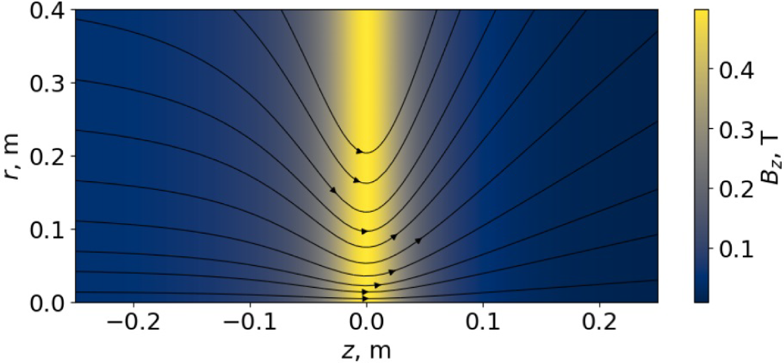
 Bz
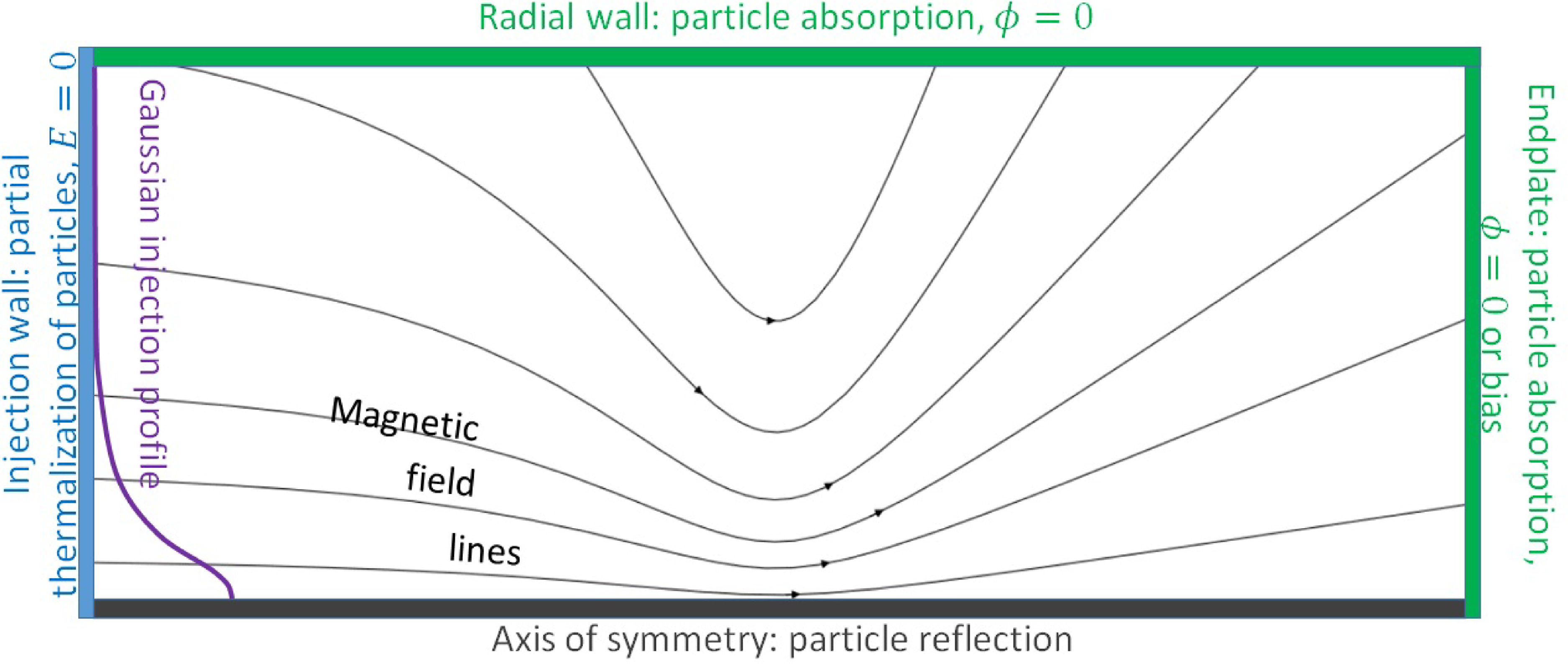
 rz
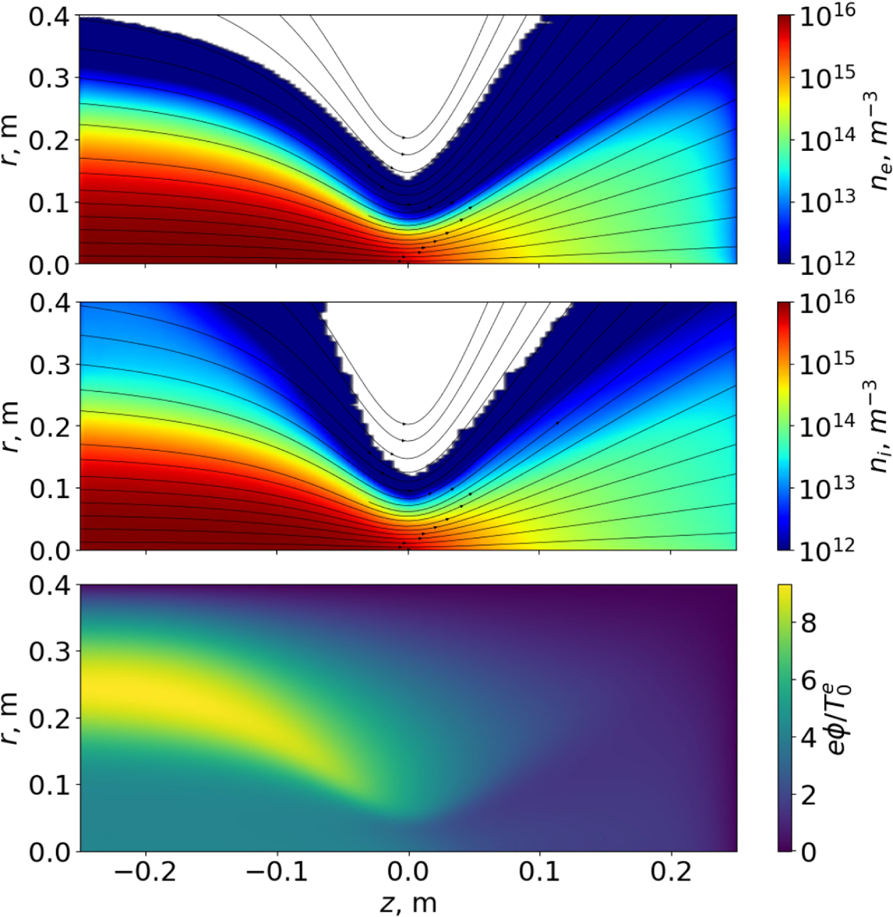
 rz
 Ti=600
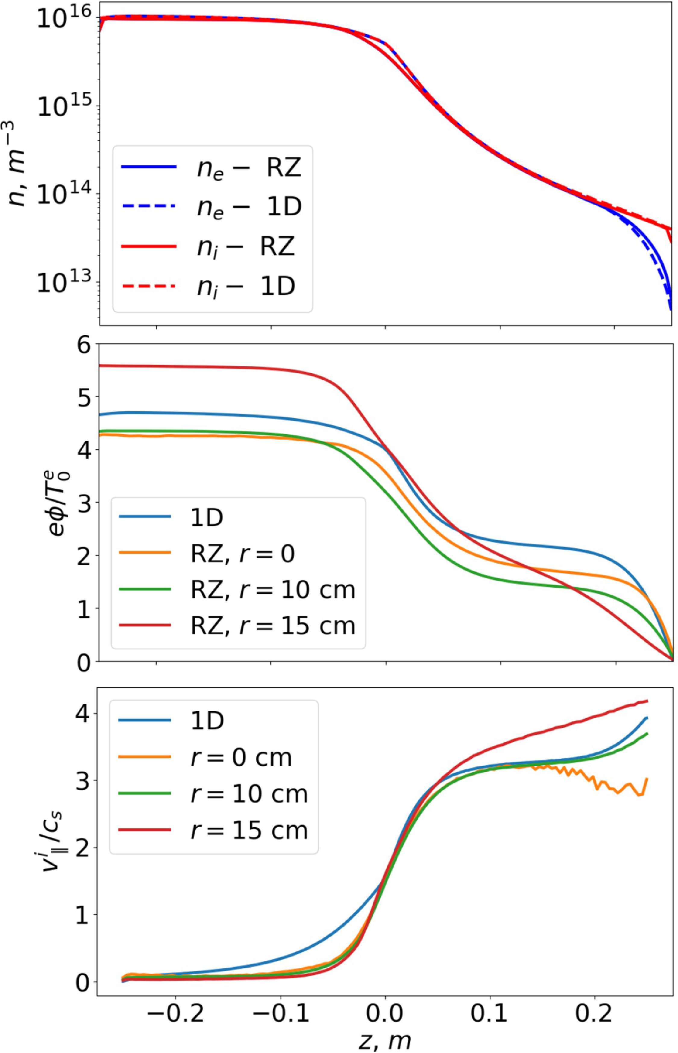
 rz
 Ti=600
 z
 z=−0.25
 rz
 r=0
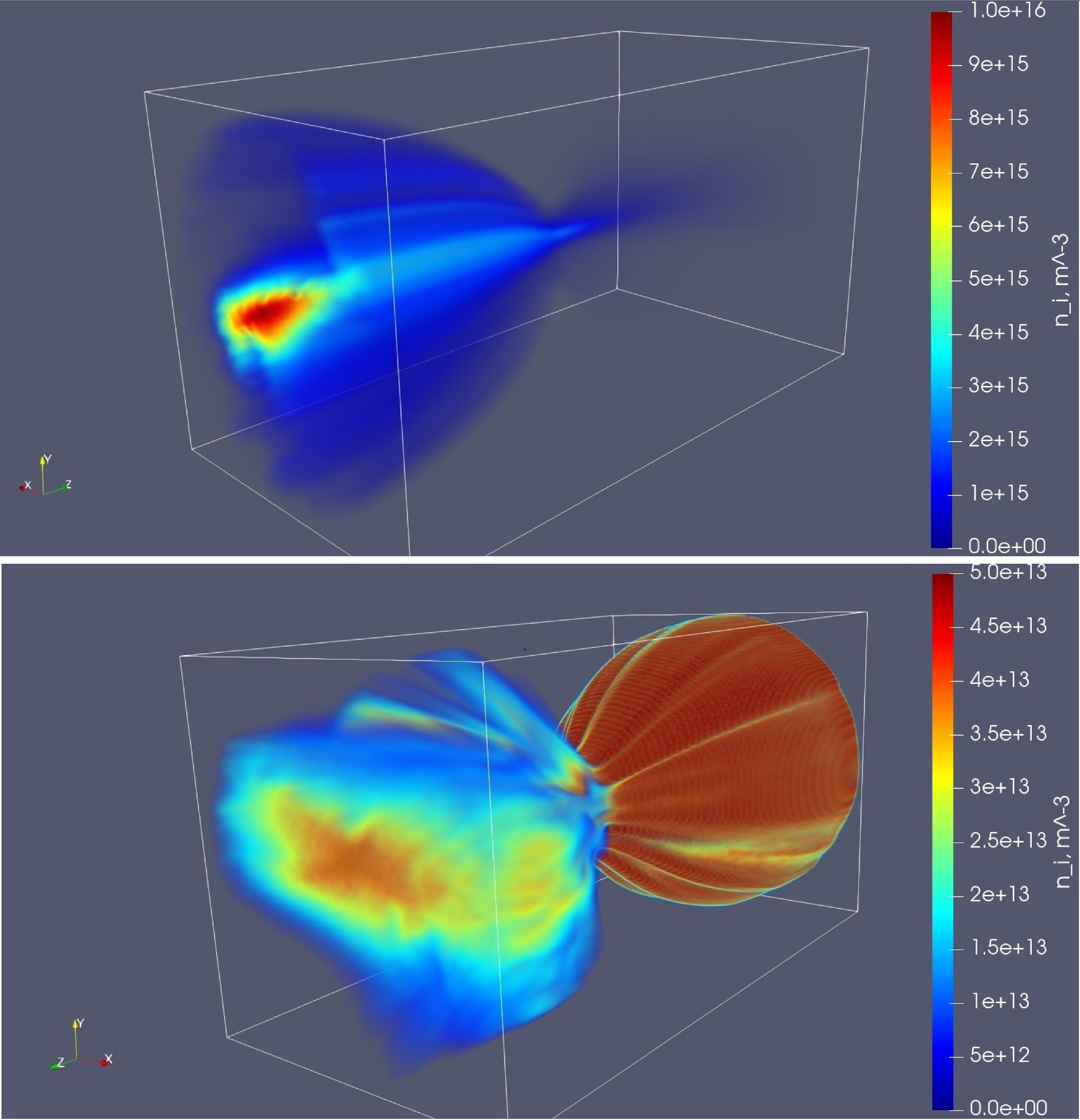
 Ti=30
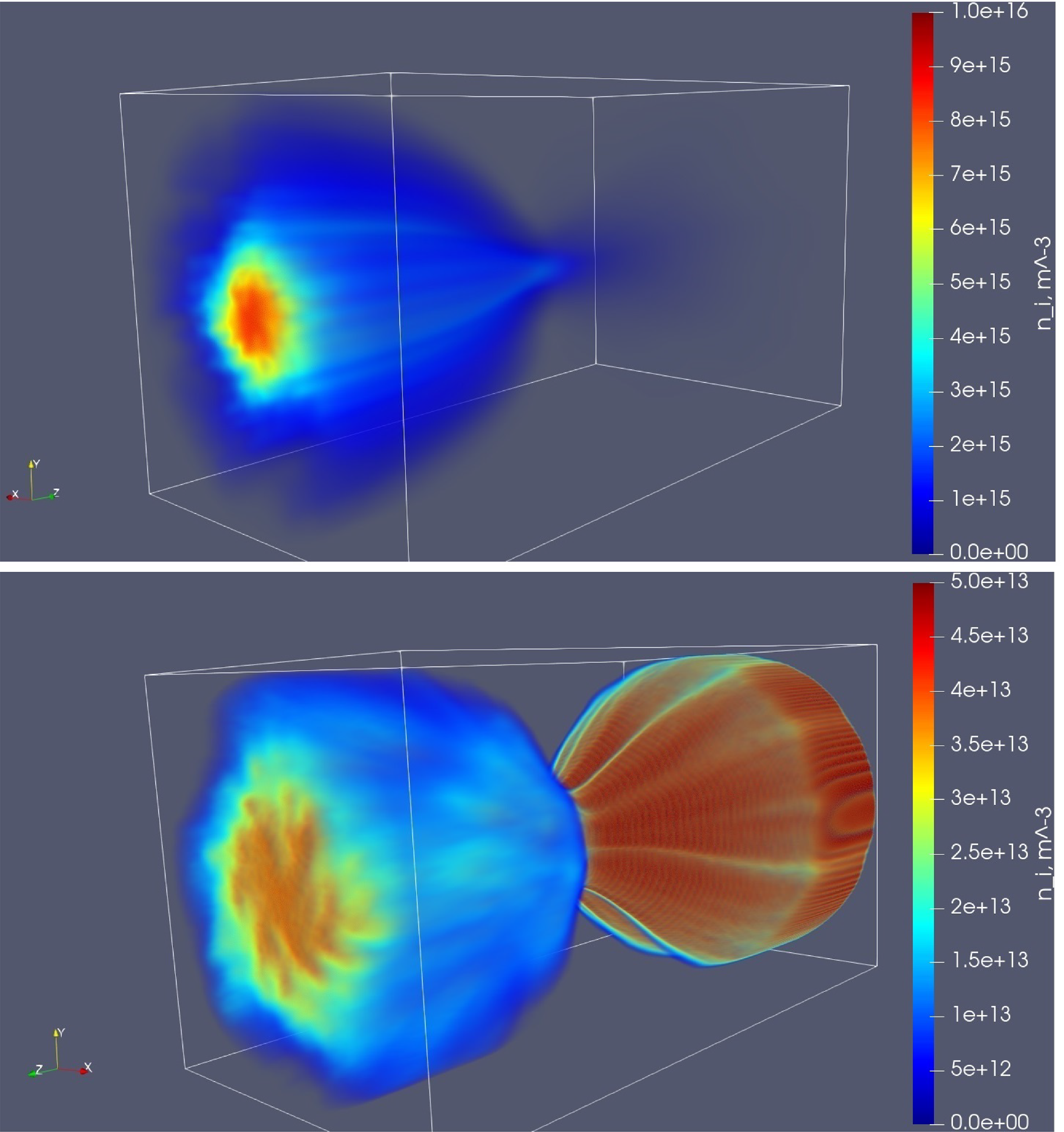
 Ti=600
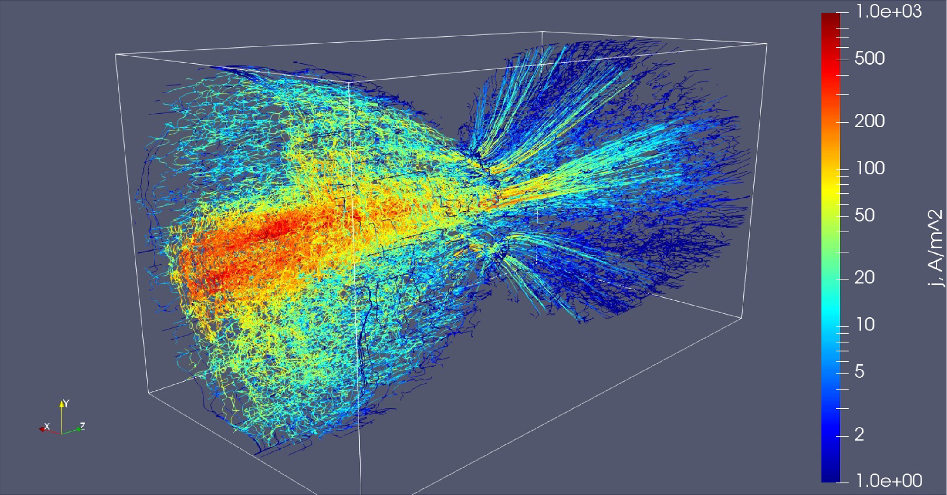
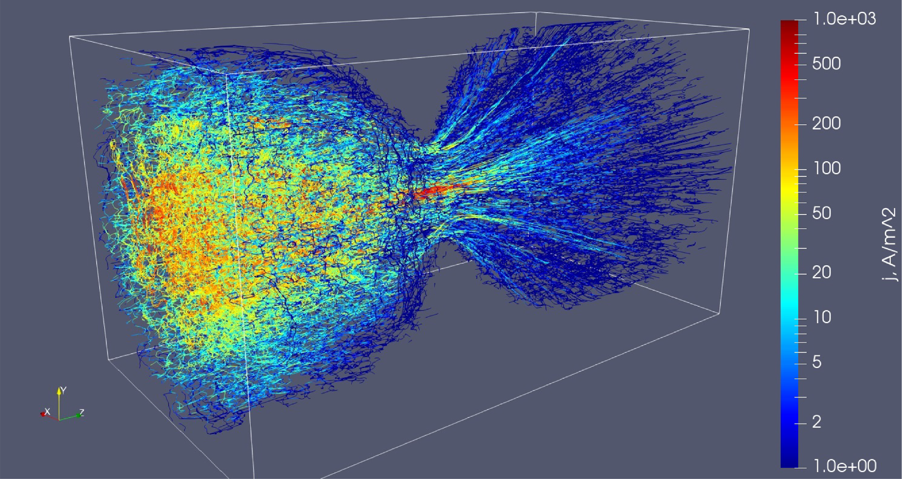
 Ti=600
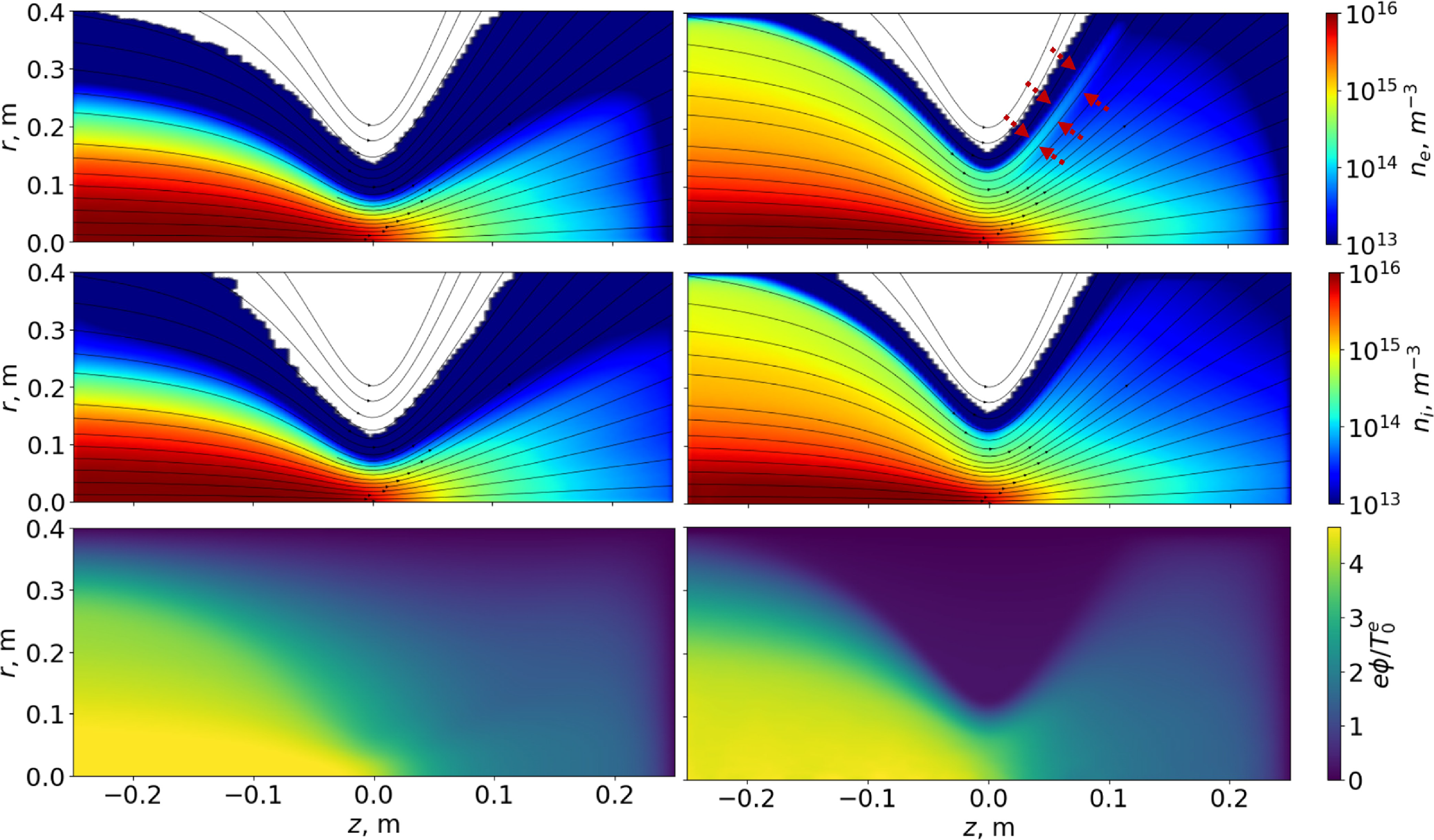
 rz
 Ti=30
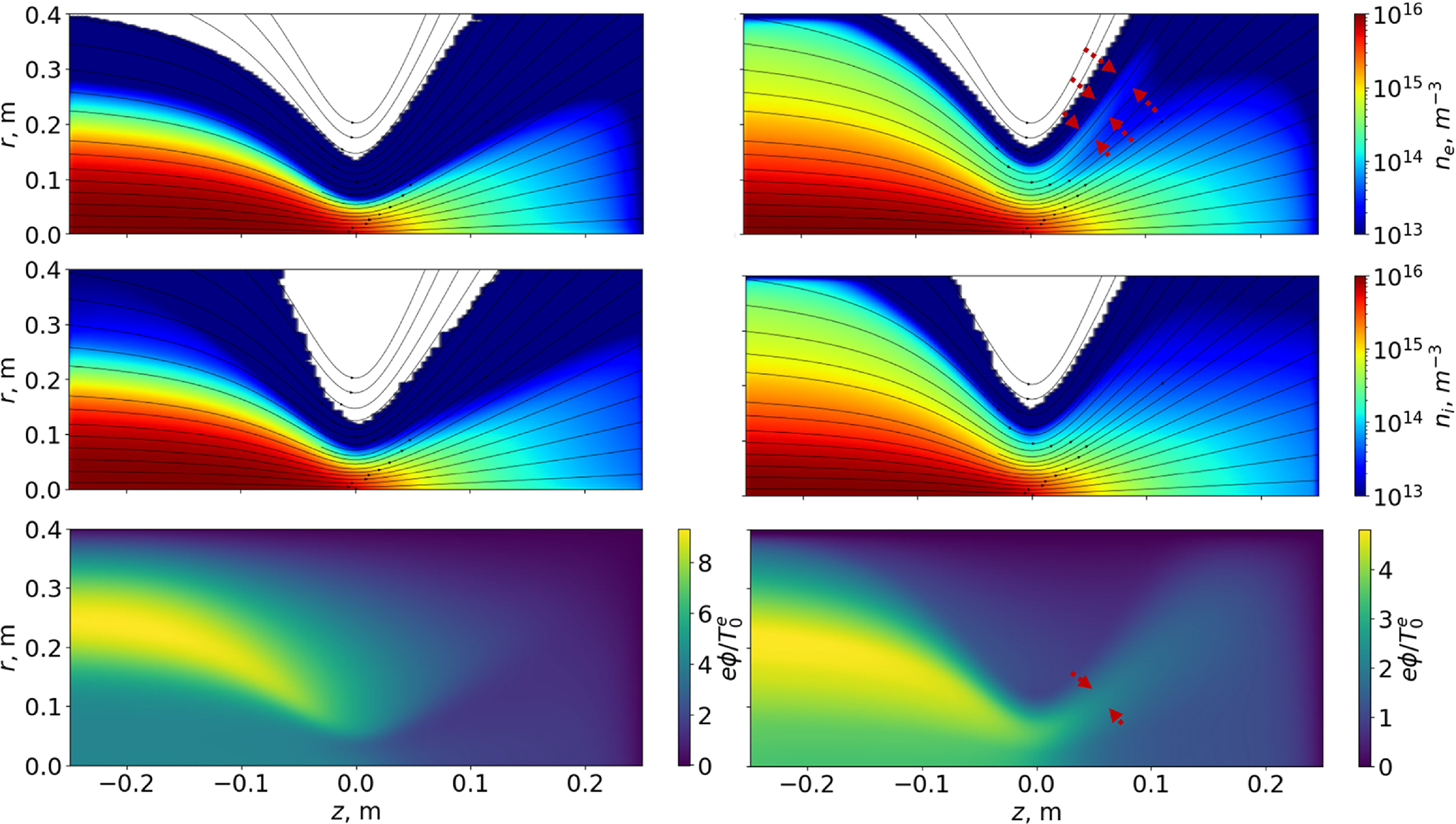
 rz
 Ti=600
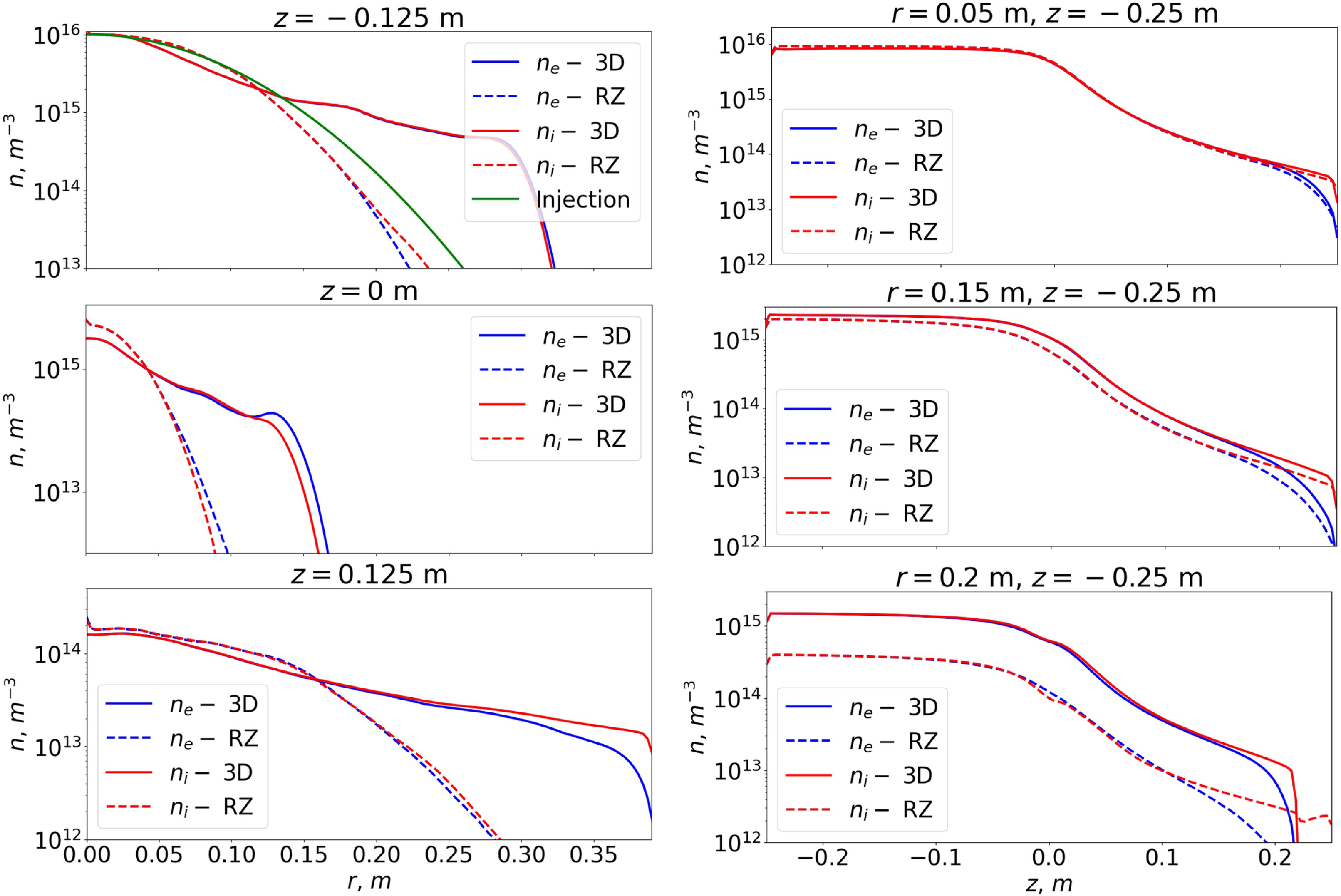
 Ti=30
 z
 n(0)=1016m−3
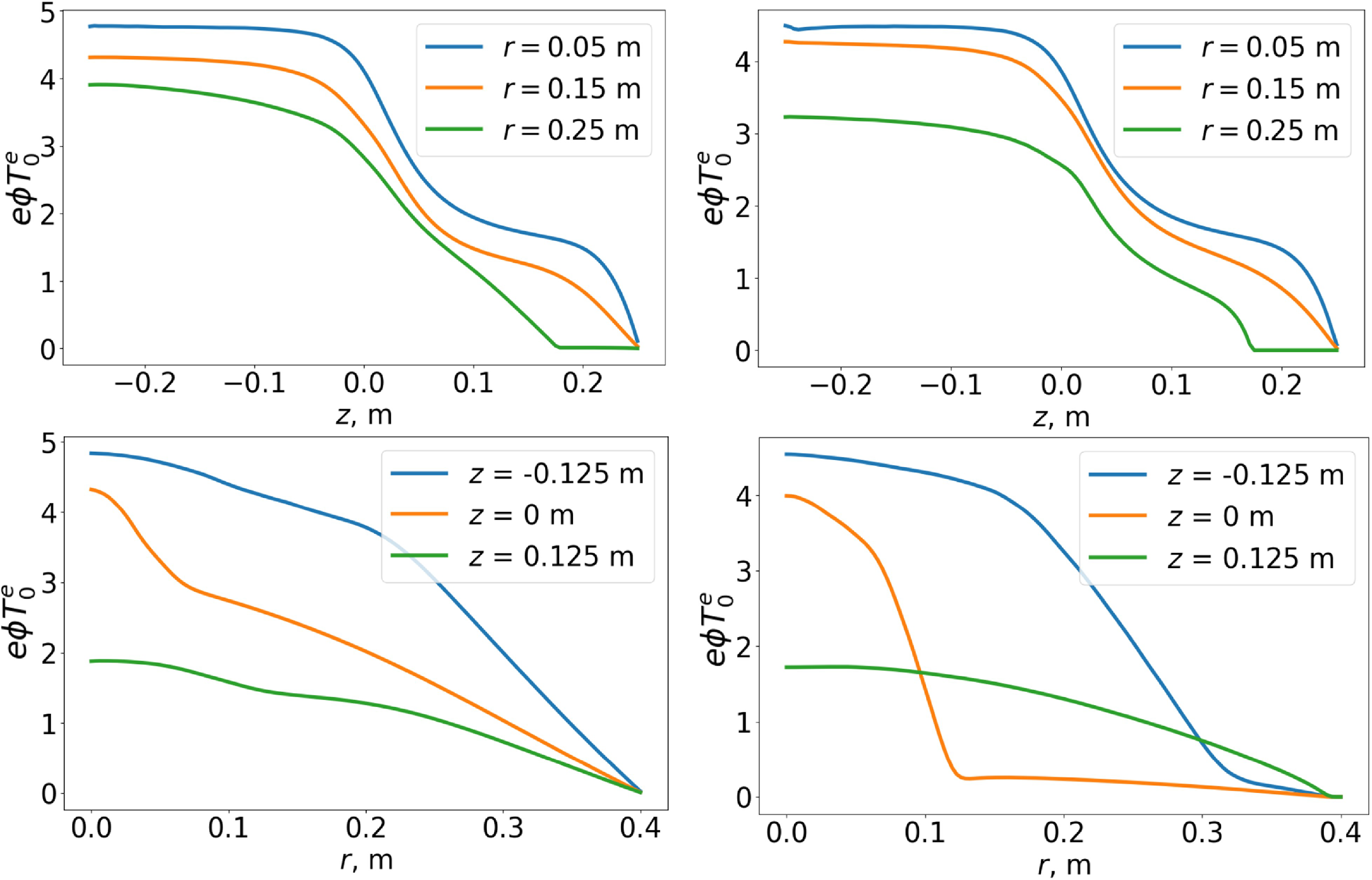
 Ti=30
 z
 rz
 z=−0.25
 r
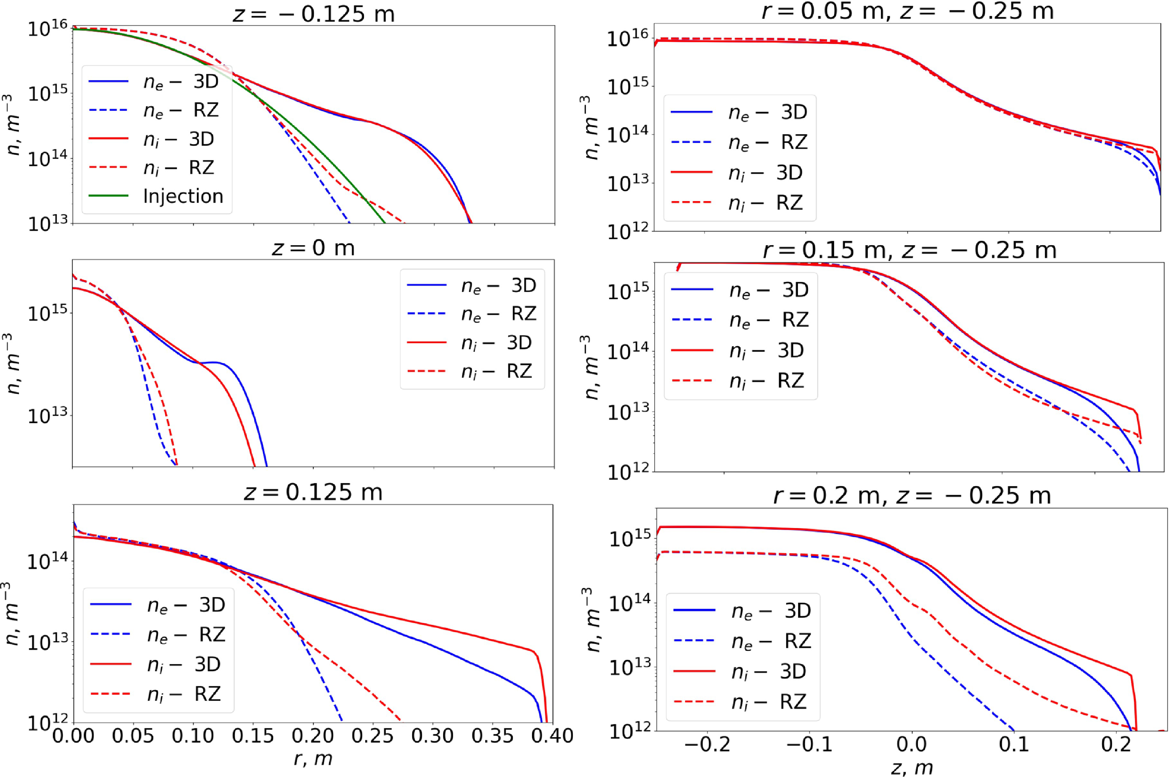
 Ti=600
 z
 r=0
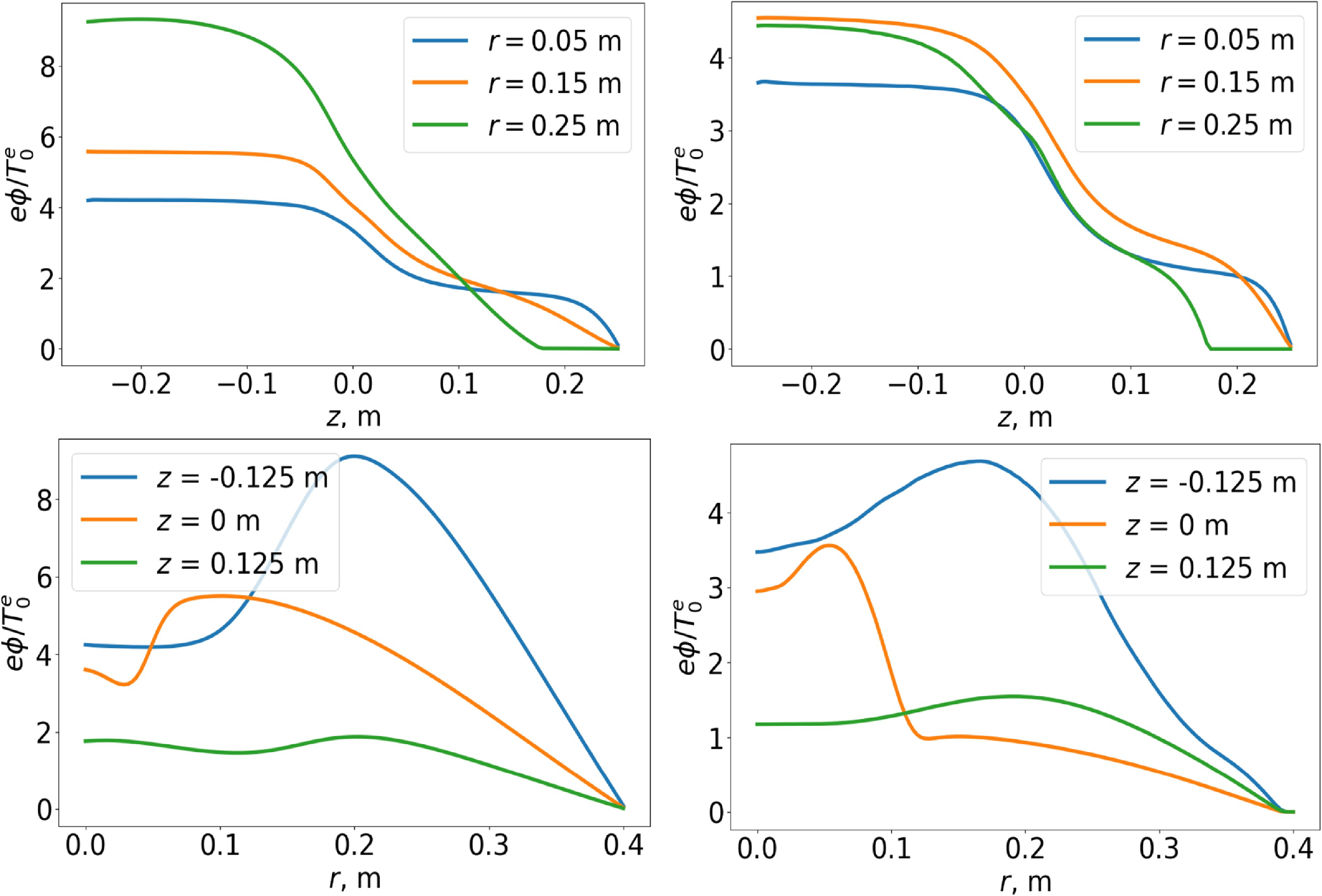
 Ti=600
 z
 rz
 z=−0.25
 r
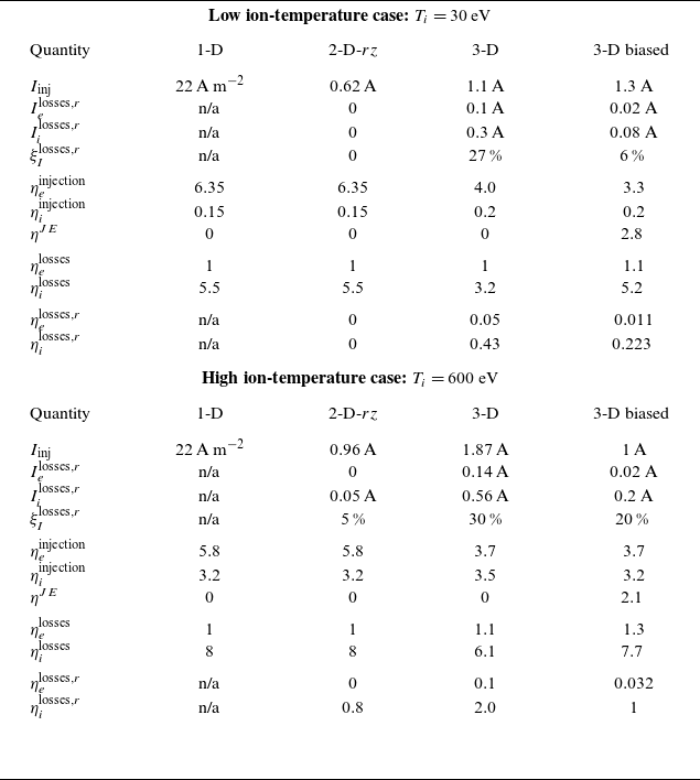
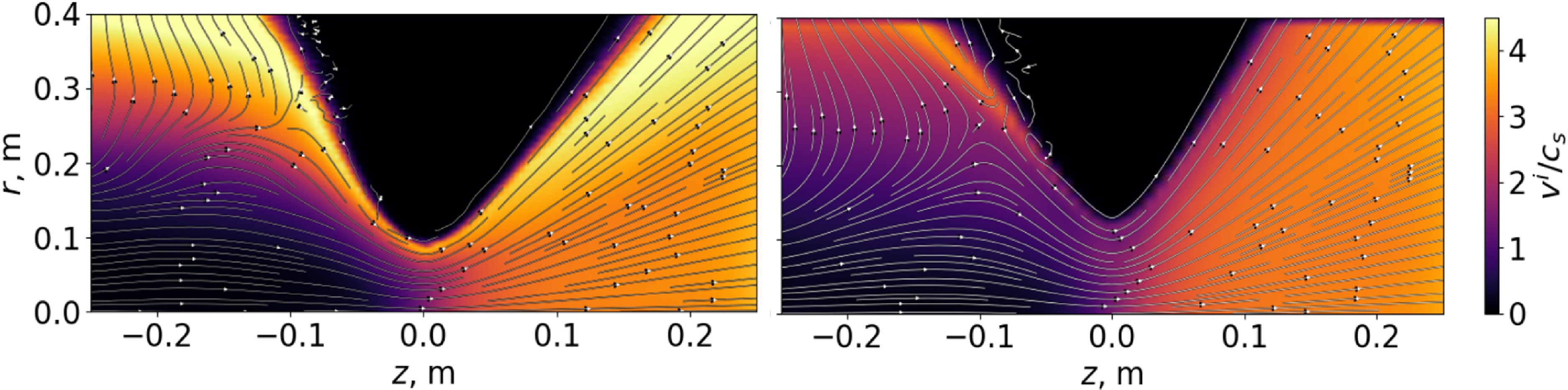
 Ti=30
 rz
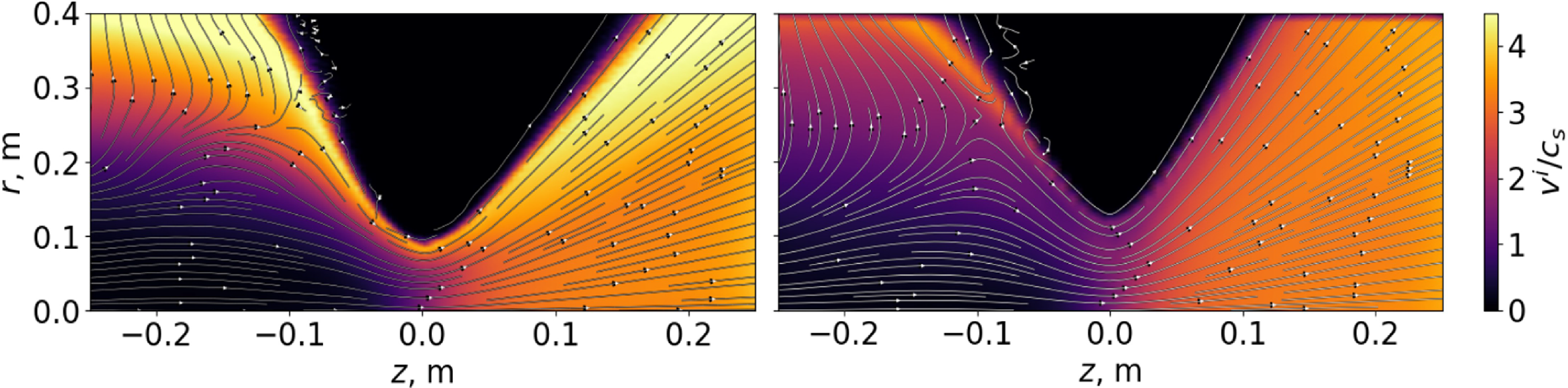
 Ti=600
 rz
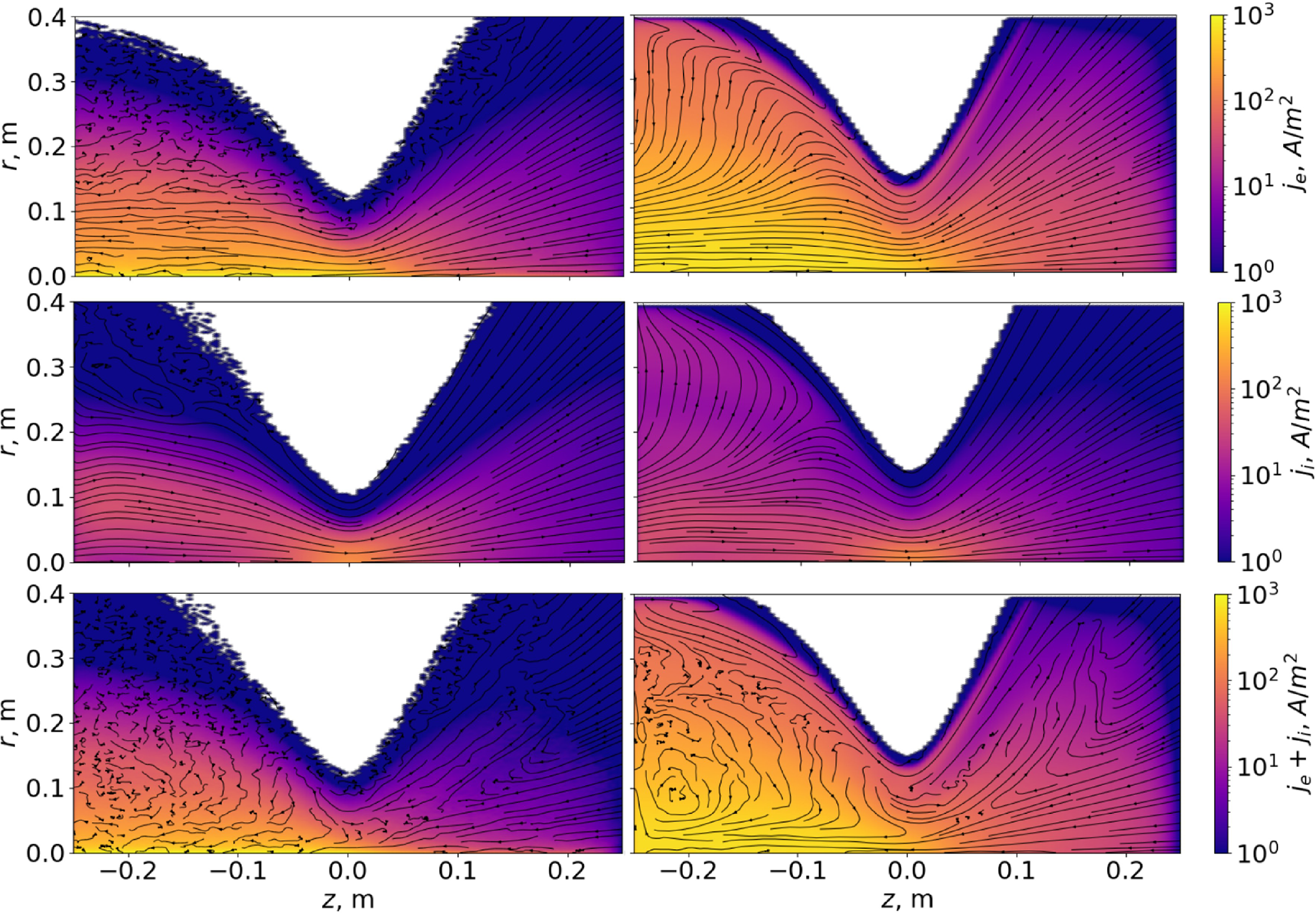
 Ti=30
 rz
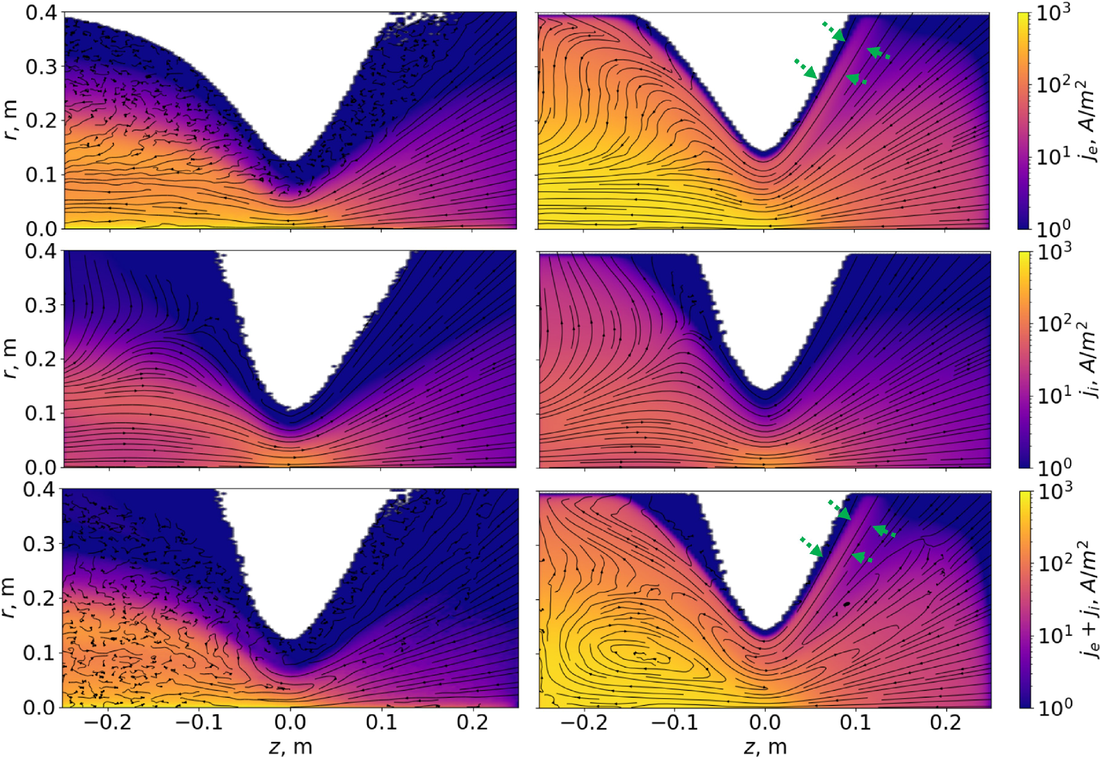
 Ti=600
 rz
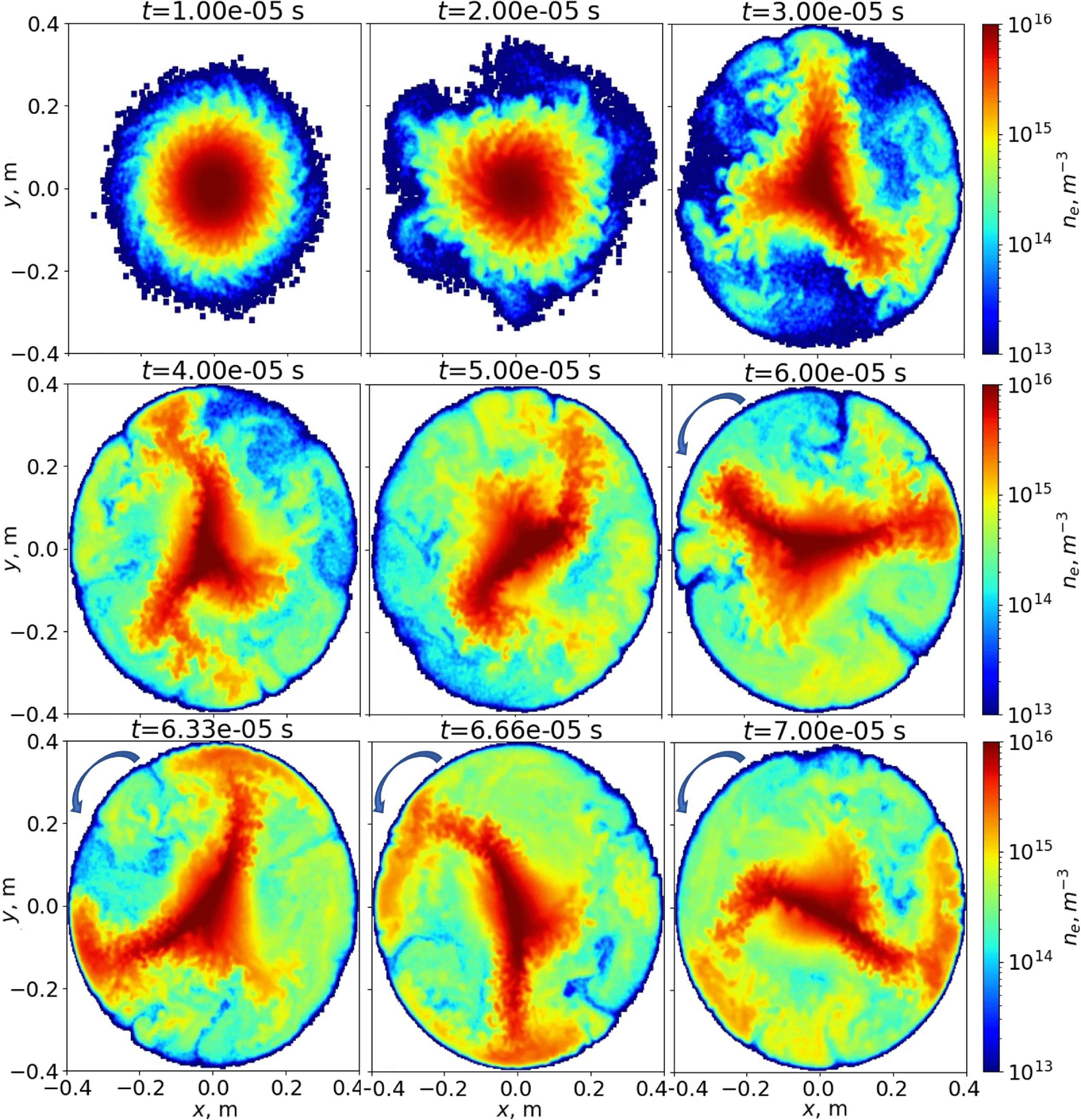
 xy
 z=−0.23
 Ti=30
 m=2
 E×B
 −z
 +z
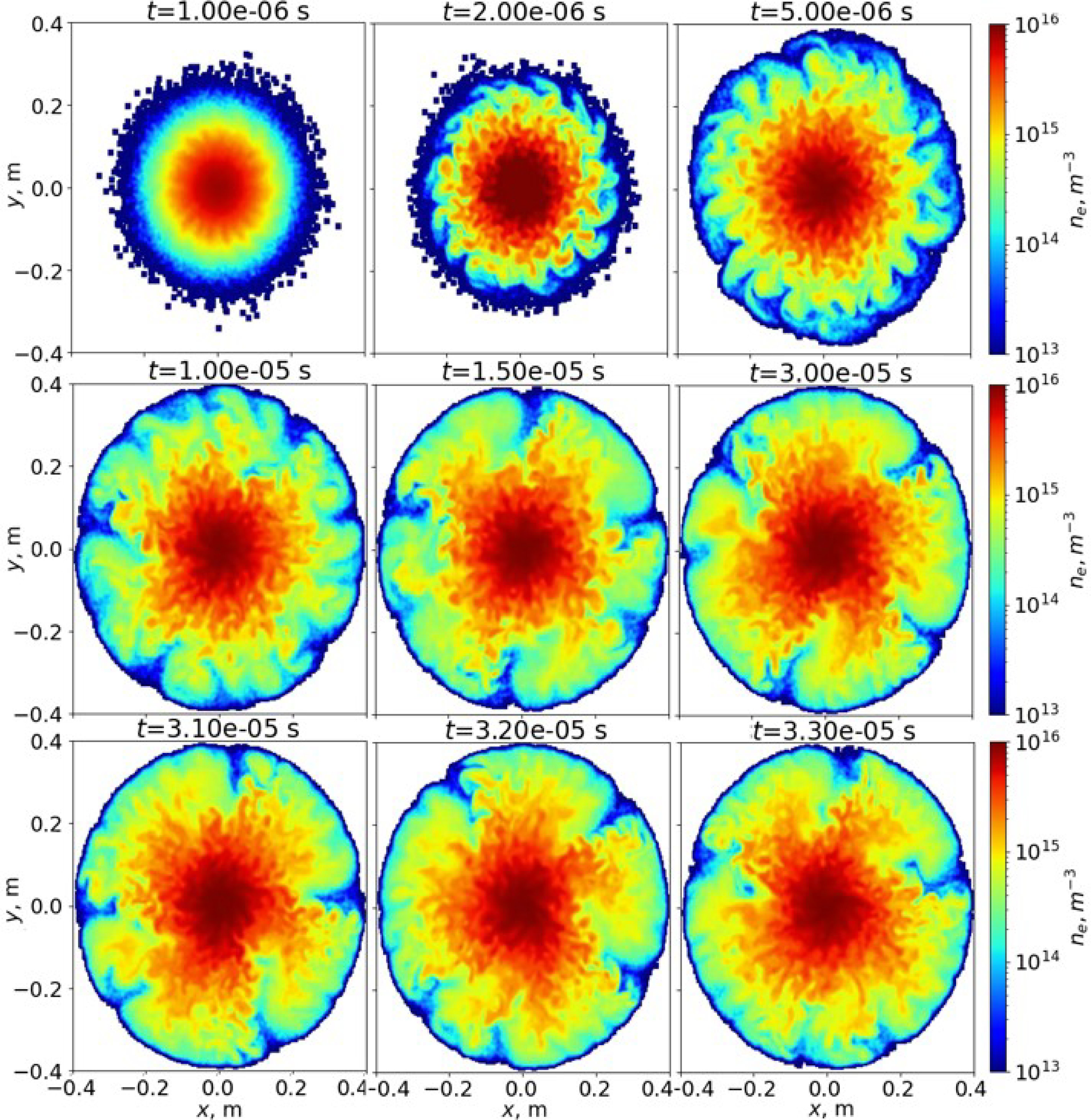
 z=−0.23
 Ti=600
 −z
 +z
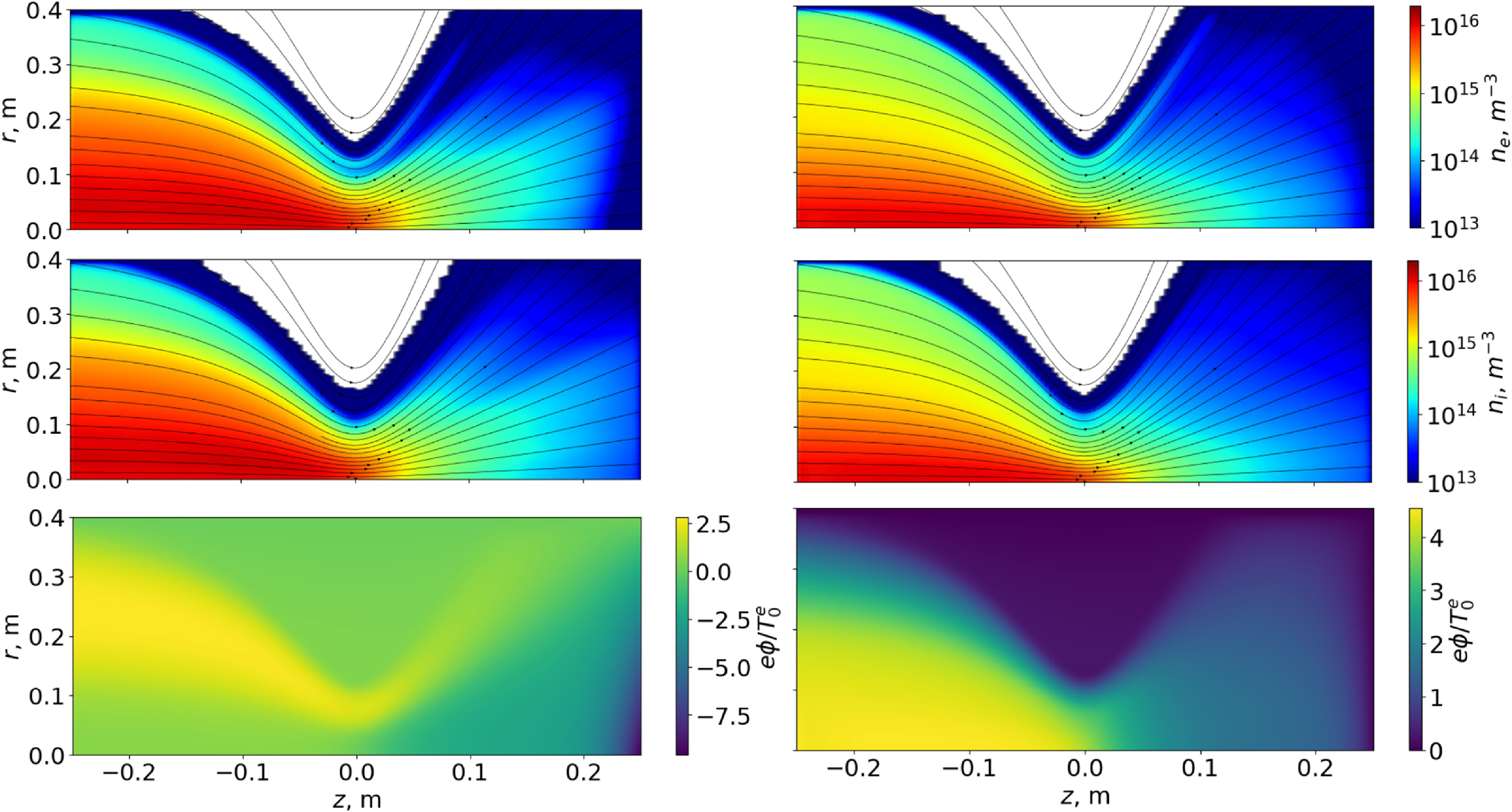
 Ti=30
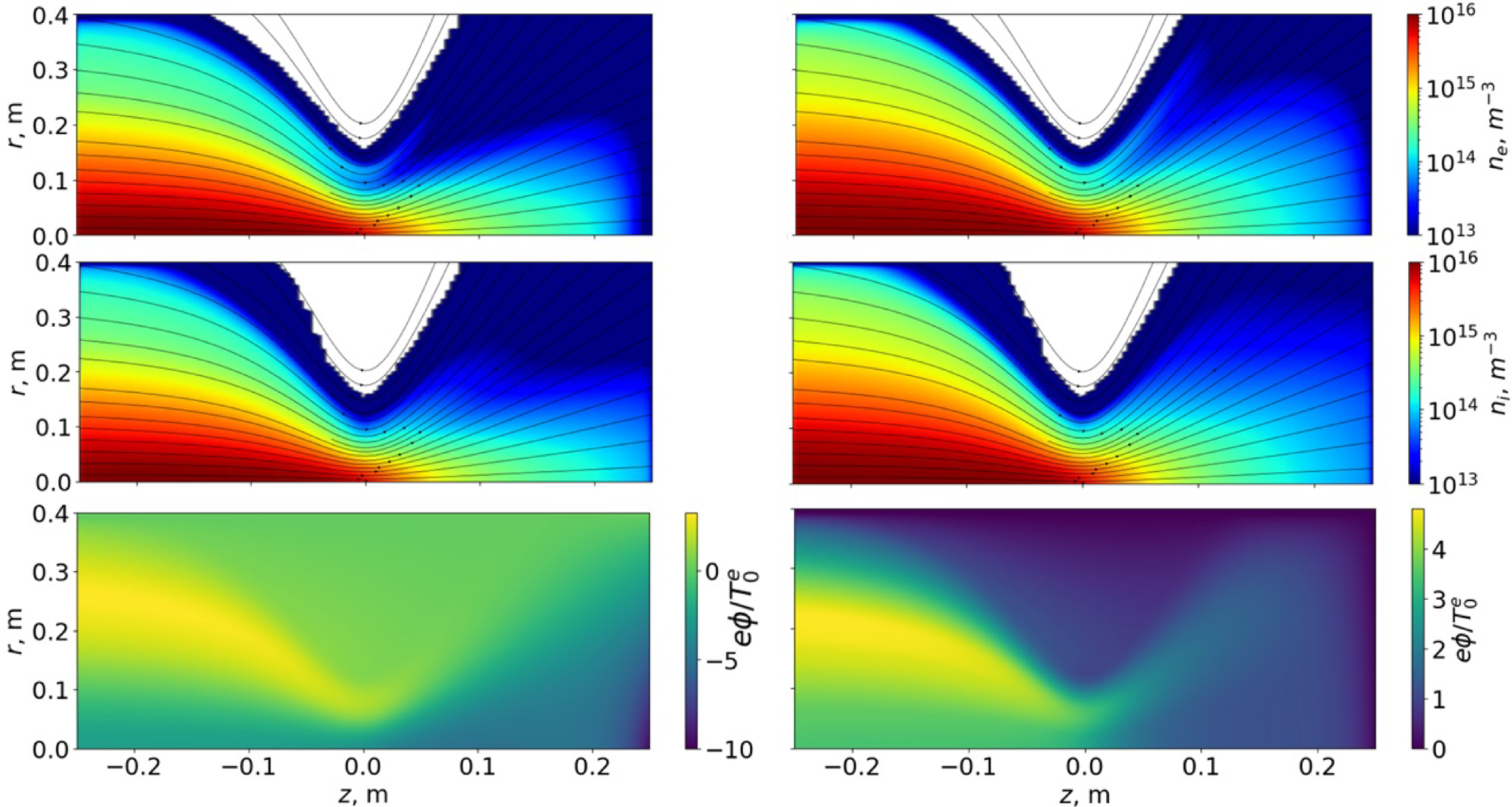
 Ti=600
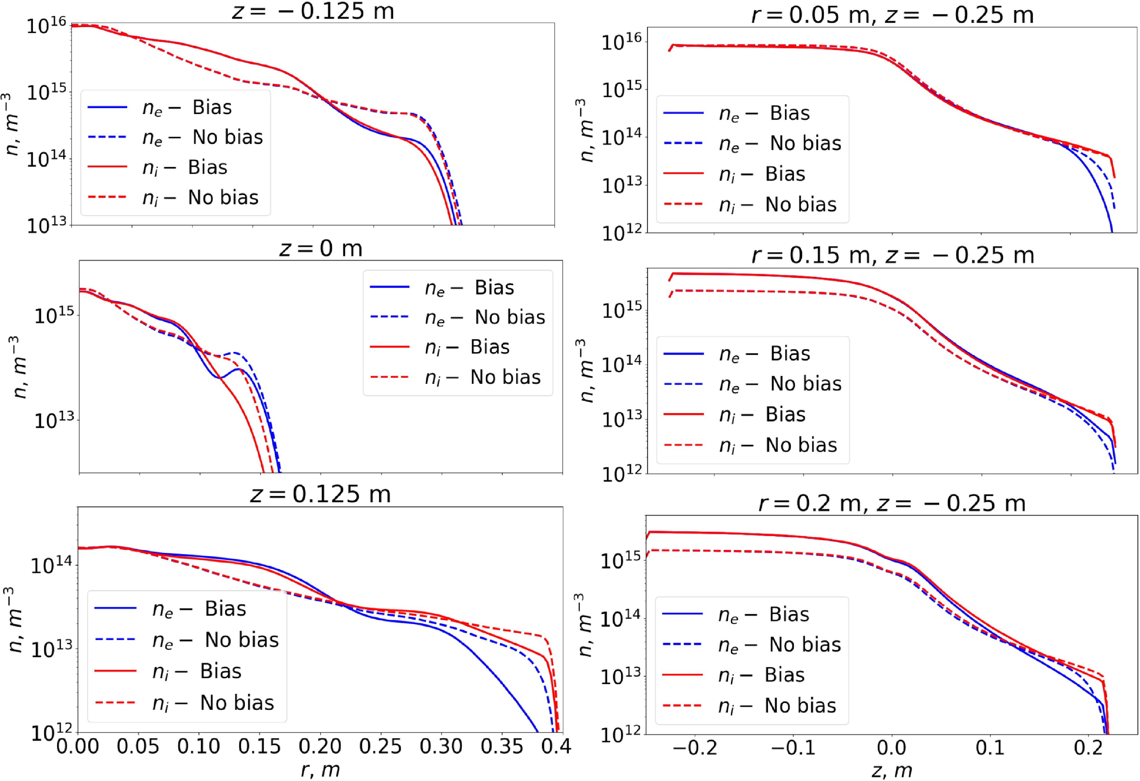
 Ti=30
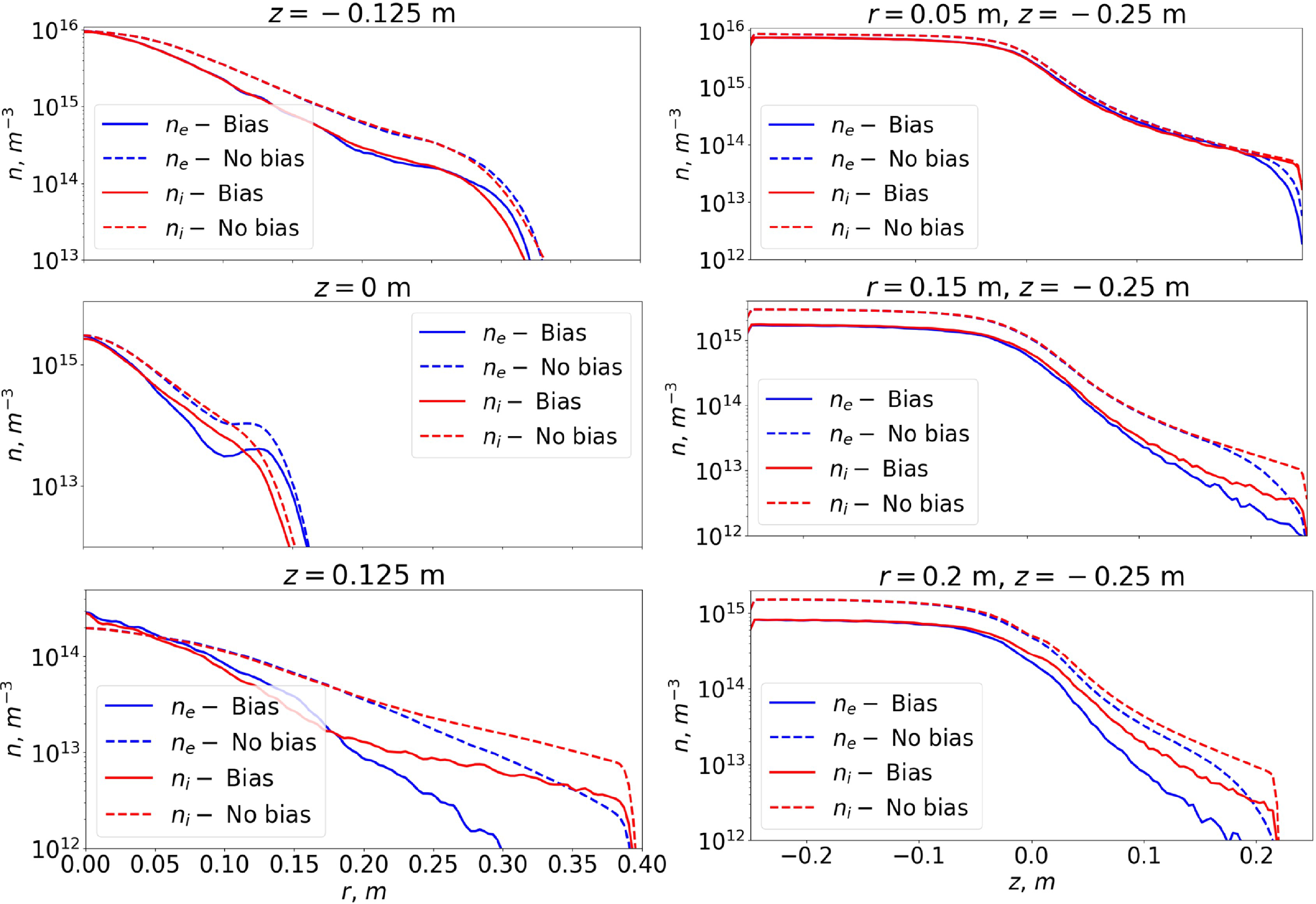
 Ti=600
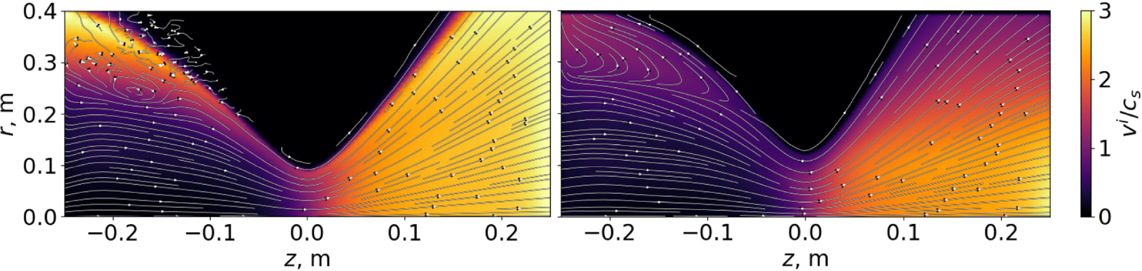
 Ti=30
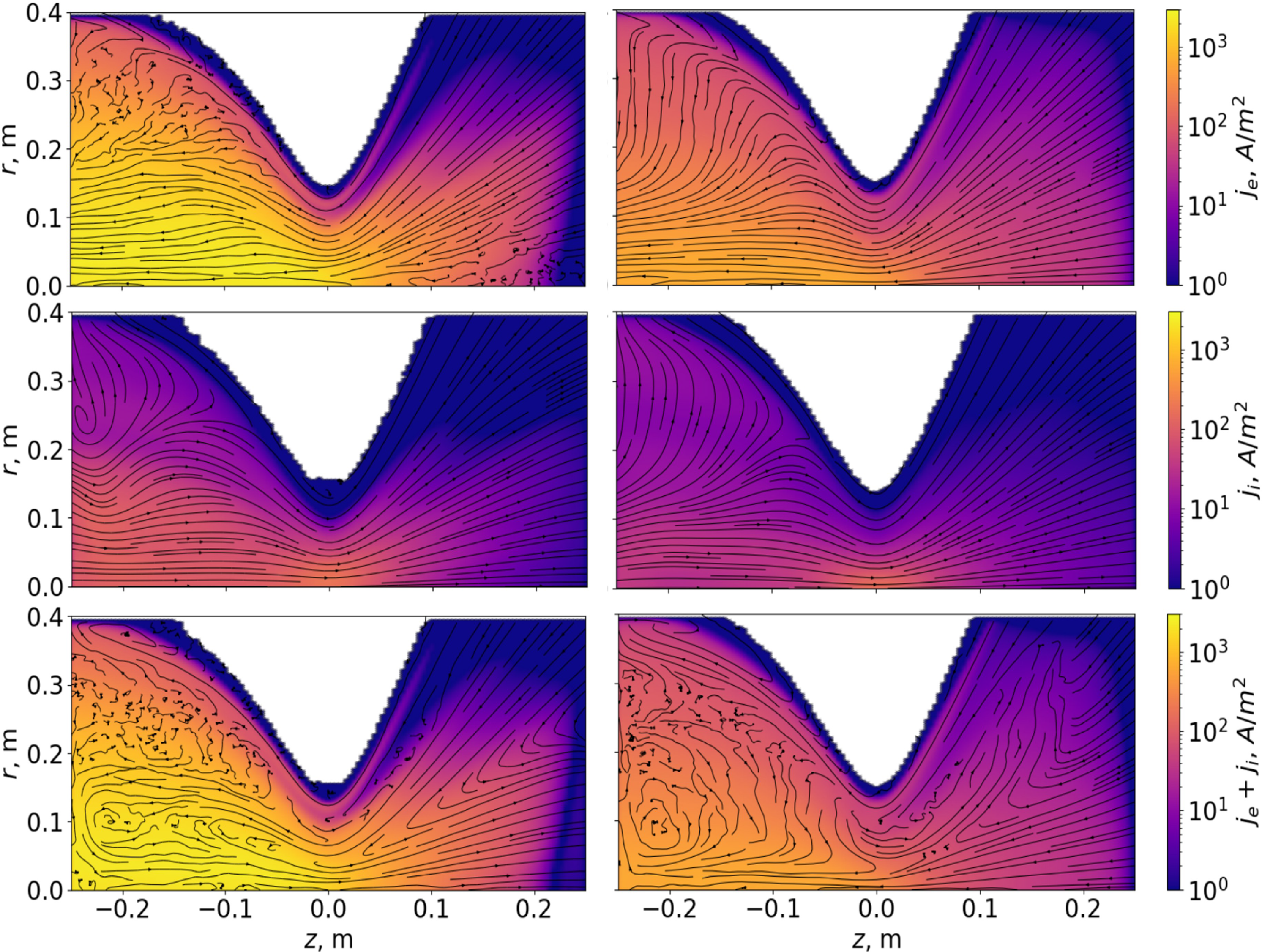
 rz
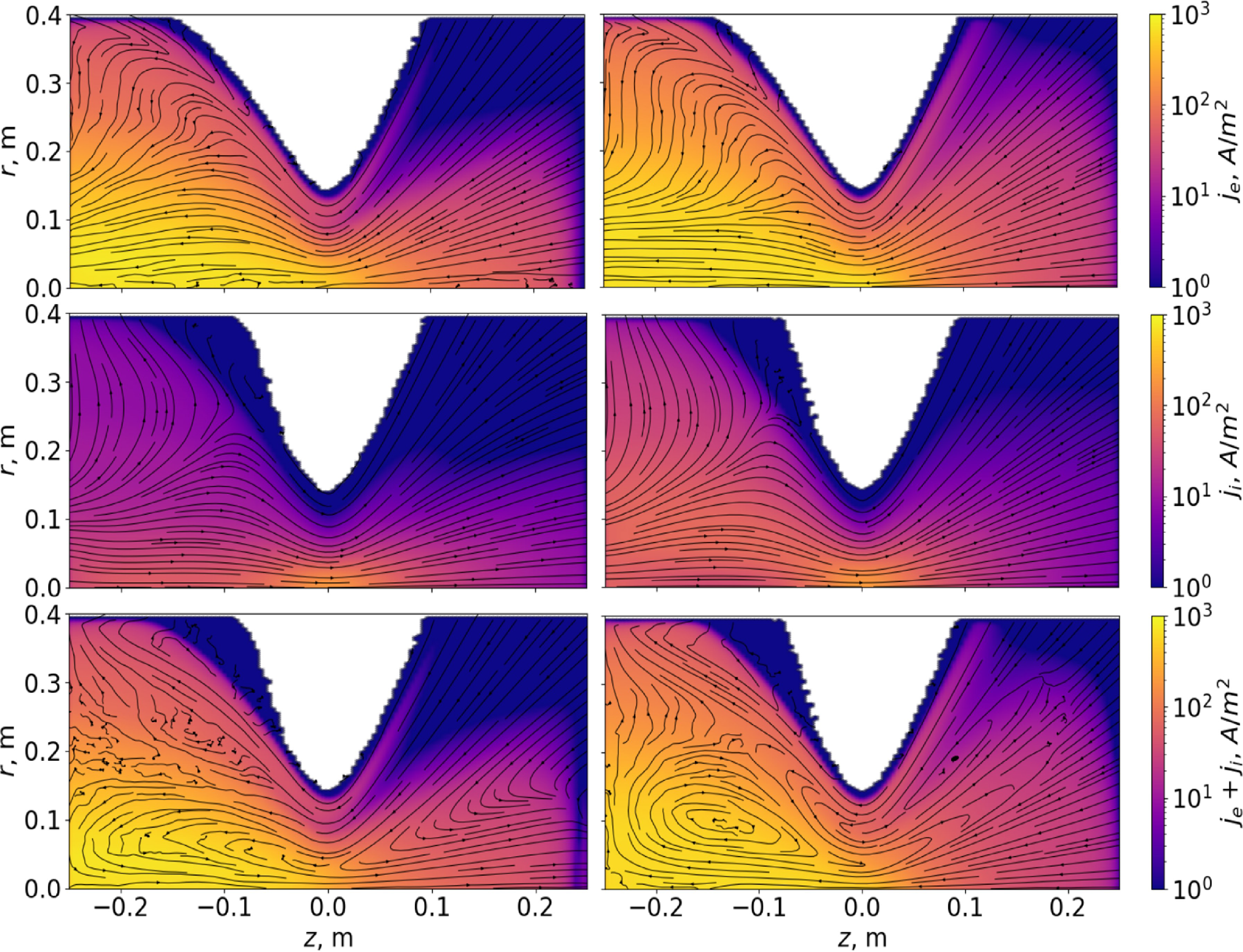
 Ti=600
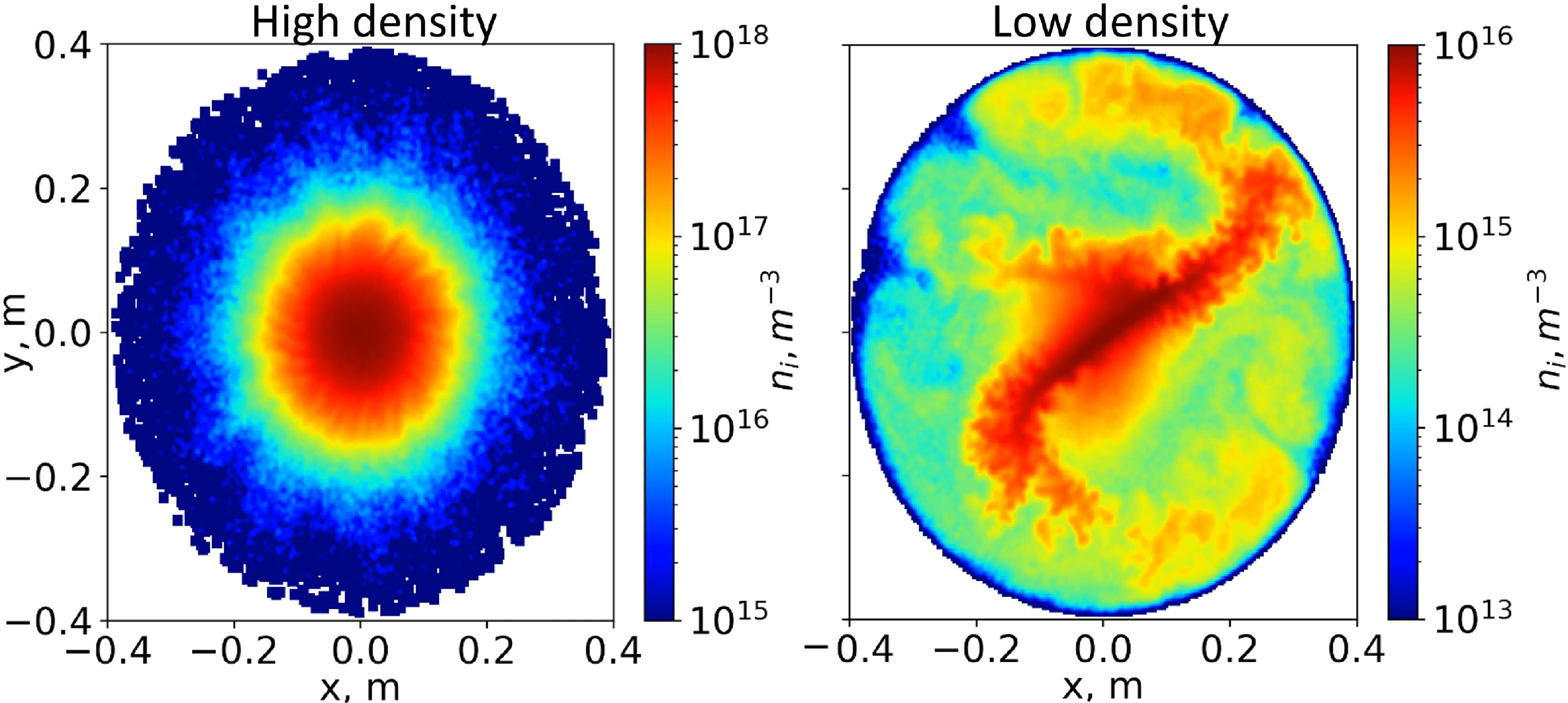
 xy
 z=−0.23
 Ti=30
 −z
 +z
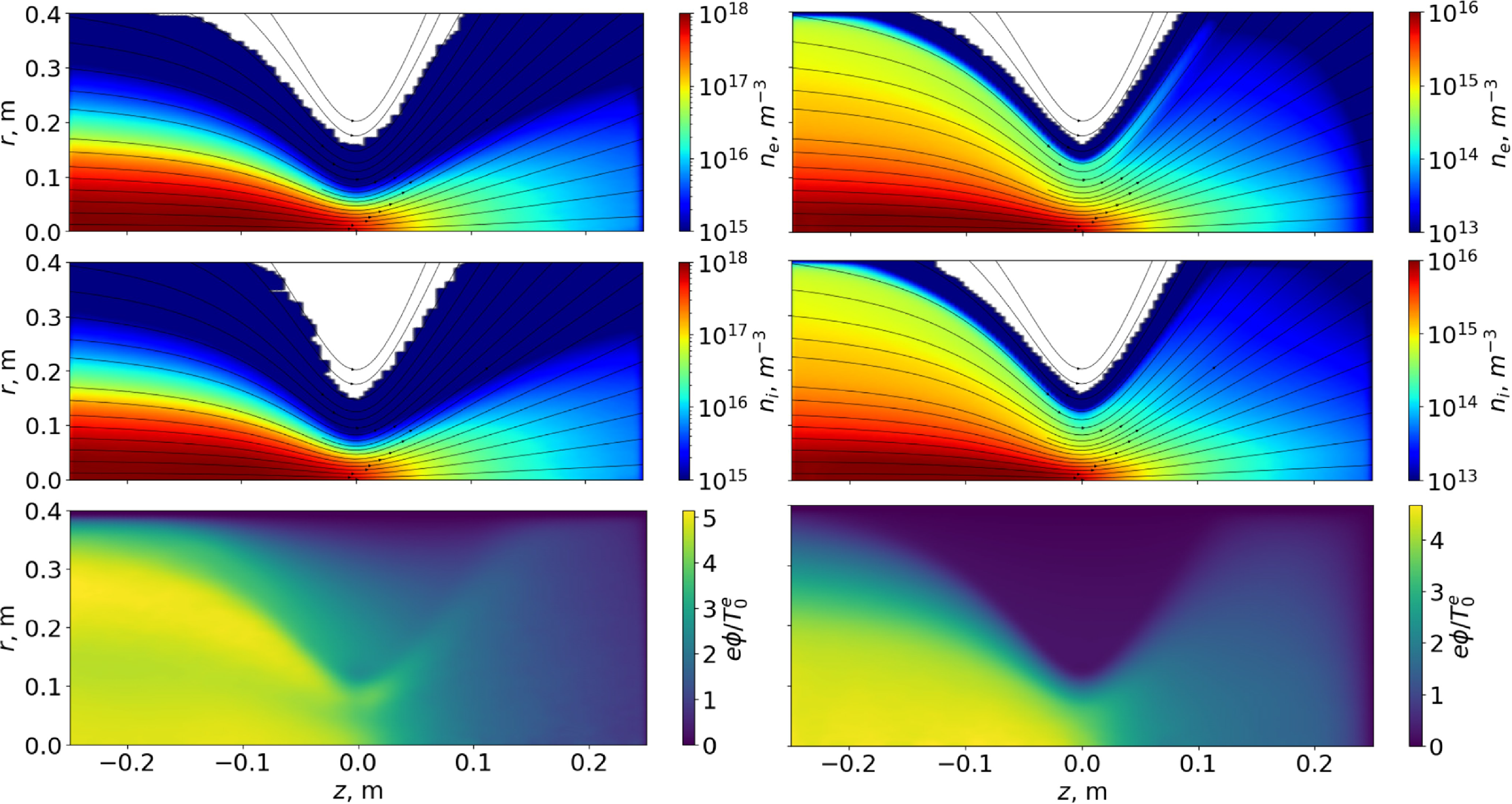
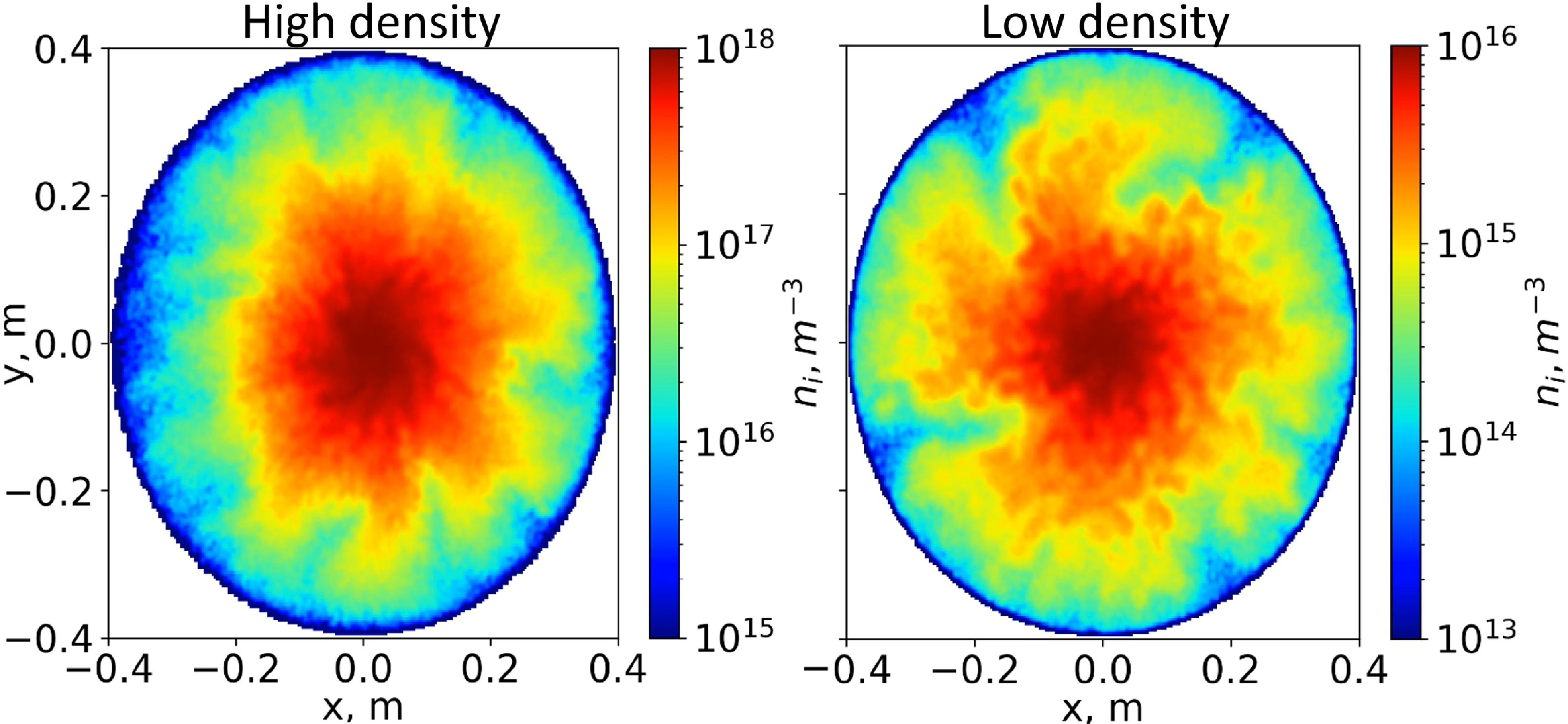
 xy
 −z
 +z
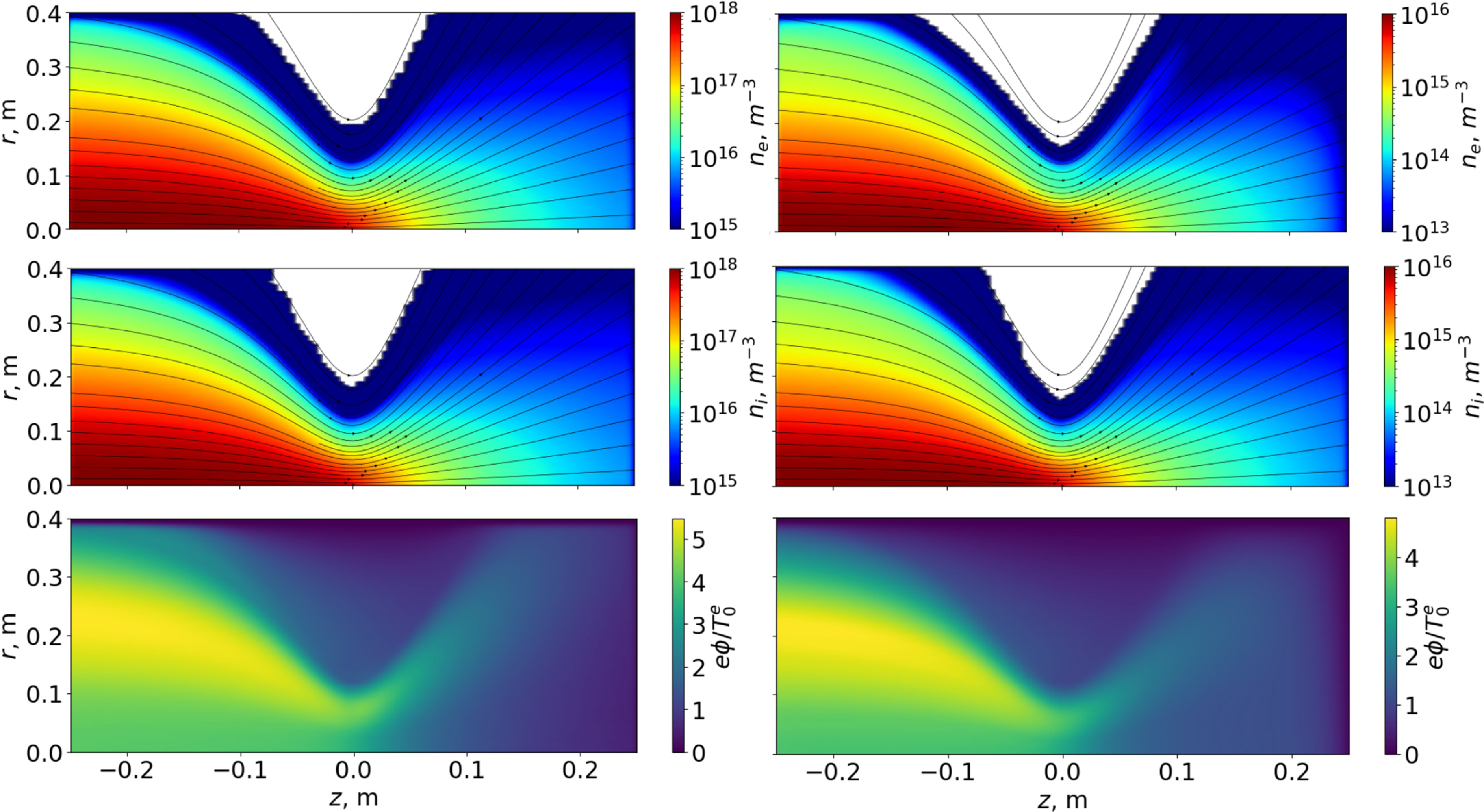


 Open access

