


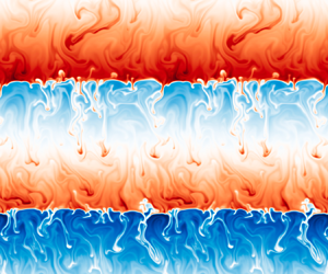
1. Introduction
Double-diffusive convection occurs when the density stratification of a gravitationally stable fluid is caused by the combination of a fast diffusing scalar and a slowly diffusing scalar of opposite contributions to the stability (Stern Reference Stern1960; Turner Reference Turner1974; Schmitt Reference Schmitt1994; Radko Reference Radko2013). In the case where the fast and slow diffuser stabilize and destabilize the fluid, respectively, the resulting instability is called ‘double-diffusive fingering’. In the opposite case, the instability is called ‘double-diffusive convection in the diffusive regime’. The necessary conditions for the fingering instability are commonly encountered in the upper layer of the tropical and subtropical ocean, where the temperature and salinity both decrease with depth (You Reference You2002), as well as in the stably stratified regions of stellar interiors (see the review by Garaud Reference Garaud2018). Fingering convection has been the object of much attention in the last 60 years, in laboratory experiments (Turner Reference Turner1967; Linden Reference Linden1973; Kunze Reference Kunze2003), theoretical models (Baines & Gill Reference Baines and Gill1969; Schmitt Reference Schmitt1979) and direct numerical simulations (Whitfield, Holloway & Holyer Reference Whitfield, Holloway and Holyer1989; Shen & Schmitt Reference Shen and Schmitt1995; Merryfield Reference Merryfield2000; Stern, Radko & Simeonov Reference Stern, Radko and Simeonov2001; Traxler et al. Reference Traxler, Stellmach, Garaud, Radko and Brummell2011; Radko & Smith Reference Radko and Smith2012). Of particular interest to the present study is the development of secondary, large-scale instabilities from a state of saturated fingering, such as thermohaline staircases (Tait & Howe Reference Tait and Howe1968; Schmitt et al. Reference Schmitt, Perkins, Boyd and Stalcup1987; Krishnamurti Reference Krishnamurti2003; Radko Reference Radko2003; Stellmach et al. Reference Stellmach, Traxler, Garaud, Brummell and Radko2011) or gravity waves (Stern Reference Stern1969; Holyer Reference Holyer1981; Traxler et al. Reference Traxler, Stellmach, Garaud, Radko and Brummell2011; Garaud et al. Reference Garaud, Medrano, Brown, Mankovich and Moore2015). The unified mean-field theory of Traxler et al. (Reference Traxler, Stellmach, Garaud, Radko and Brummell2011), following the pioneering efforts of Radko (Reference Radko2003), introduced a general formalism containing all previous theories on large-scale double-diffusive instabilities. However, the theory was originally developed with oceanographic applications in mind, i.e. for the heat-salt system, and therefore does not include settling of one of the scalar fields. The particular case where suspended particles, or sediment, play the role of the slow diffuser is referred to as sedimentary fingering convection (Houk & Green Reference Houk and Green1973). While qualitatively similar to traditional double-diffusive convection (Green Reference Green1987), sedimentary fingering exhibits unique dynamics (Sánchez & Roget Reference Sánchez and Roget2007; Burns & Meiburg Reference Burns and Meiburg2012; Yu, Hsu & Balachandar Reference Yu, Hsu and Balachandar2013, Reference Yu, Hsu and Balachandar2014; Burns & Meiburg Reference Burns and Meiburg2015; Davarpanah Jazi & Wells Reference Davarpanah Jazi and Wells2016; Alsinan, Meiburg & Garaud Reference Alsinan, Meiburg and Garaud2017; Reali et al. Reference Reali, Garaud, Alsinan and Meiburg2017). The work of Reali et al. (Reference Reali, Garaud, Alsinan and Meiburg2017) was the first and (to the best of the authors’ knowledge) the only study to investigate the effect of settling on mean-field instabilities. These authors restricted their analysis to the study of layering instabilities. They found that settling has two complementary effects on layer formation. First, they showed that the settling-induced phase shift between the particle field and the scalar field drives a new mean-field layering instability that is unique to double-diffusive settling. Second, they showed that in some cases, settling can modify the fingering turbulence enough to make it unstable to layering in the traditional sense of Radko (Reference Radko2003). Possible evidence for settling-driven layering was presented in the work of Carazzo & Jellinek (Reference Carazzo and Jellinek2013), who investigated layer formation in volcanic ash clouds by conducting idealized laboratory experiments in particle-laden salt-stratified water. Their results motivated the theory of Reali et al. (Reference Reali, Garaud, Alsinan and Meiburg2017) at the time, and while the exact mechanism by which layers form in these experiments remains unclear, the possibility of further experiments using a similar set-up prompts us to perform a more comprehensive study of mean-field instabilities in particle-driven double-diffusive convection.
Here, we extend the works of Traxler et al. (Reference Traxler, Stellmach, Garaud, Radko and Brummell2011) and Reali et al. (Reference Reali, Garaud, Alsinan and Meiburg2017) to create a unified mean-field theory for large-scale instabilities in sedimentary double-diffusive convection. This unified theory recovers previous mean-field theory results of Stern et al. (Reference Stern, Radko and Simeonov2001); Radko (Reference Radko2003); Traxler et al. (Reference Traxler, Stellmach, Garaud, Radko and Brummell2011) and Reali et al. (Reference Reali, Garaud, Alsinan and Meiburg2017) in various limits. (Traxler et al. (Reference Traxler, Stellmach, Garaud, Radko and Brummell2011) further considered lateral gradients, thus allowing their theory to also recover the Walsh & Ruddick (Reference Walsh and Ruddick1995) theory of intrusions.) As we shall demonstrate, our work reveals the existence of a new settling-driven collective instability that differs from Stern's particle-free collective instability. Section 2 describes the modelling approach. Section 3 presents the generalized stability analysis of small-scale and mean-field modes. In § 4, we discuss the stability of non-sedimentary systems in the high-Prandtl-number regime and conduct direct numerical simulations (DNS) of a representative problem. In § 5, we analyse the stability of sedimentary systems in the high-Prandtl-number regime and provide a physical interpretation of the new settling-driven collective instability. We validate our results, at least qualitatively, against DNS. Section 6 concludes with a discussion of the main findings, and how they relate to realistic flows in natural settings.
2. Modelling approach
2.1. Governing equations
We model the system using the two-dimensional Navier–Stokes equations in the Boussinesq approximation. Following the same framework as Alsinan et al. (Reference Alsinan, Meiburg and Garaud2017) and Reali et al. (Reference Reali, Garaud, Alsinan and Meiburg2017), we begin by assuming that the particle concentration field can be modelled as a continuum. We then use the equilibrium Eulerian formalism in which the velocity of the particle field  $u_p^*$ is related to the dimensional fluid velocity field
 $\boldsymbol {u}^*$ (where the asterisk superscript denotes dimensional variables), via
 \begin{equation} \boldsymbol{u}_p^* = \boldsymbol{u}^* -V_{st}\boldsymbol{e}_y, \end{equation}
where  $V_{st}$ is the constant dimensional Stokes settling velocity and
 $\boldsymbol {e}_y$ is the upward vertical unit vector. For sufficiently spherical particles of density
 $\rho _p\gg \rho _f$ and radius
 $R$,
 \begin{equation} V_{st} = \frac{2}{9}\frac{(\rho_p - \rho_f )}{\rho_f }\frac{gR^2}{\nu}. \end{equation}
where  $g$ is the gravitational acceleration and
 $\nu$ is the kinematic viscosity. The equilibrium Eulerian formalism applies to particulate flows with Stokes number
 $St = {\tau _p}/{\tau _e}\ll 1$, where
 $\tau _p = V_{st}/g$ is the particle stopping time and
 $\tau _e=U_{rms}/l$ is the eddy turnover time, with
 $U_{rms}$ the root-mean-square (r.m.s.) eddy velocity and
 $l$ the characteristic eddy size (Ferry & Balachandar Reference Ferry and Balachandar2001; Rani & Balachandar Reference Rani and Balachandar2003). Thus, the applicability of the formalism can only be verified a posteriori, and is discussed for relevant parameters in § 6. We further assume that the particle concentration field, denoted by
 $C^*$, can be written as the sum of a time-dependent background
 $C_0^*(y^*,t^*) = C_m + C_{0y}(y^* + V_{st}^*)$, where
 $C_m$ is a mean reference density and
 $C_{0y}$ is the constant background vertical gradient, plus perturbations
 $\tilde {C}^*$, as
 \begin{equation} C^*(x^*,y^*,t^*) =C_0^*(y^*,t^*) + \tilde{C}^*(x^*,y^*,t^*). \end{equation}
These particles are embedded in a fluid that is salt stratified, with a constant background vertical gradient of salinity  $S_{0y}$, and with perturbations
 $\tilde {S}^*$ from that background, so the total salinity field is
 \begin{equation} S^*(x,y,t) = S_{0}^*(y^*) + \tilde{S}^*(x^*,y^*,t^*), \end{equation}
where  $S_0^*(y^*) = S_m + y^* S_{0y}$ and
 $S_m$ is a reference salinity. Finally, we use the Boussinesq approximation to relate the total density
 $\rho ^*$ to the salinity and particle concentration as
 \begin{equation} \frac{\rho^* - \rho_0^*}{\rho_f} = \alpha (S^* - S^*_0) + \beta (C^* - C^*_0), \end{equation}
where  $\rho _f$ is the mean fluid density,
 $\rho _0^*(y^*,t^*)$ is the total density of a fluid of salinity
 $S_0^*(y^*)$ and particle concentration
 $C_0^*(y^*,t^*)$, and
 $\alpha$ and
 $\beta$ are constant coefficients related to derivatives of the equation of state. The set of governing equations is given by
 \begin{gather} \boldsymbol{\nabla}^* \boldsymbol{\cdot} \boldsymbol{u}^* = 0, \end{gather}
 \begin{gather} \frac{\partial \boldsymbol{u}^*}{\partial t^*} + (\boldsymbol{u}^* \, {\boldsymbol\cdot} \, \boldsymbol\nabla^*) \boldsymbol{u}^* = -\frac{1}{\rho_f}\boldsymbol{\nabla}^* \tilde{p}^* + \nu\Delta^* \boldsymbol{u}^* - (\alpha \tilde{S}^* + \beta \tilde{C}^* )g\boldsymbol{e}_y, \end{gather}
 \begin{gather} \frac{\partial \tilde{C}^*}{\partial t^*} + \boldsymbol{u}^* \boldsymbol{\cdot} \boldsymbol{\nabla}^* \tilde{C}^* + \tilde{v}^* C_{0y}- V_{st}\frac{\partial \tilde{C}^*}{\partial y^*} = \kappa_c \Delta^* \tilde{C}^*, \end{gather}
 \begin{gather} \frac{\partial \tilde{S}^*}{\partial t^*} + \boldsymbol{u}^* \boldsymbol{\cdot} \boldsymbol{\nabla}^* \tilde{S}^* + \tilde{v}^* S_{0y} = \kappa_s\Delta^* \tilde{S}^*. \end{gather}
where  $\boldsymbol {u}^* = (u^*,v^*)$,
 $\tilde {p}^*$ is the dimensional pressure perturbation from the background state,
 $\boldsymbol {g} = -g\boldsymbol {e}_y$ is the acceleration due to gravity (
 $g\approx 9.81\ \mathrm {m}\,\mathrm {s}^{-2}$),
 $\nu$ is the kinematic viscosity (
 $\nu \approx 10^{-6}\ \mathrm {m}^2\,\mathrm {s}^{-1}$) and
 $\kappa _s$ and
 $\kappa _c$ are the salt and particle diffusivities, respectively. While the molecular diffusivity of salt ions is typically
 $\kappa _s\approx 10^{-9} \ \mathrm {m}^2\,\mathrm {s}^{-1}$ (Poisson & Papaud Reference Poisson and Papaud1983), the hydrodynamic diffusivity of particles is more difficult to characterize as it varies markedly with the hydrodynamic conditions of the suspension, the shear experienced by the particles, the particle volume fraction, as well as the size of the particles (Davis Reference Davis1996). However, for very small and non-inertial particles that thus fall within the limits of applicability of the equilibrium Eulerian description of particle transport, the particle diffusivity is very small and
 $\kappa _c/\kappa _s\ll 1$. We note that this assumption breaks down when hard boundaries are present in the fluid domain and particles are allowed to accumulate, and that the suspension is therefore not locally dilute. Here, however, all perturbations to the background state are assumed to be doubly periodic, to eliminate any contamination by boundary conditions.
2.2. Non-dimensional equations
The governing equations (2.6)–(2.9) are made non-dimensional using the anticipated finger scale  $d = ({\nu \kappa _s}/{\alpha g | S_{0y}|})^{{1}/{4}}= ({\nu \kappa _s}/{N^2})^{{1}/{4}}$, following standard practice (Radko Reference Radko2013), where
 $N$ is the local buoyancy frequency associated with the salt stratification. A velocity scale
 $U ={\kappa _s}/{d}$ and time scale
 $T = {d^2}/{\kappa _s}$ are then introduced based on the diffusivity of the fast diffuser. The salinity and particle concentration fields are non-dimensionalized using
 $d| S_{0y}|$ and
 $({\alpha }/{\beta })d| S_{0y}|$ respectively. By choosing
 $P = \rho _f \nu \kappa _s/d^2$ as the pressure scale, the non-dimensional equations become
 \begin{gather} \boldsymbol{\nabla} \boldsymbol{\cdot} \boldsymbol{u} = 0, \end{gather}
 \begin{gather} \frac{1}{Pr}\left(\frac{\partial \boldsymbol{u}}{\partial t} + (\boldsymbol{u} \boldsymbol{\cdot} \boldsymbol{\nabla}) \boldsymbol{u} \right)= -\boldsymbol{\nabla} \tilde{p} + \Delta \boldsymbol{u} - \left(\tilde{S} + \tilde{C}\right)\boldsymbol{e}_y, \end{gather}
 \begin{gather} \frac{\partial \tilde{C}}{\partial t} + \boldsymbol{u} \boldsymbol{\cdot} \boldsymbol{\nabla} \tilde{C} +\frac{v}{R_0}- V\frac{\partial \tilde{C}}{\partial y} = \tau \Delta\tilde{C},\end{gather}
 \begin{gather} \frac{\partial \tilde{S}}{\partial t} + \boldsymbol{u} \boldsymbol{\cdot} \boldsymbol{\nabla} \tilde{S} -v= \Delta \tilde{S}, \end{gather}
where all quantities have now been non-dimensionalized, and where  $\tau = {\kappa _c}/{\kappa _s}$ is the diffusivity ratio,
 $Pr = {\nu }/{\kappa _s}$ (
 $\approx 10^{3}$) is the Prandtl number (although it is understood here as a Schmidt number, we choose to call it a Prandtl number in order to stay consistent with the existing literature on double diffusion, which is mainly focused on heat-salt systems) and
 $V = {V_{st}d}/{\kappa _s}$ is the non-dimensional settling velocity. The density ratio is
 $R_0 = {\alpha | S_{0y}|}/{\beta | C_{0y}|}$.
The system (2.10)–(2.13) is identical to that of Alsinan et al. (Reference Alsinan, Meiburg and Garaud2017), with the only exception that the authors considered a temperature–particle system. This impacts the signs of the dimensional background gradients  $S_{0y}$ and
 $C_{0y}$, leading to sign differences in the non-dimensional perturbation equations. For consistency with the literature (Traxler et al. Reference Traxler, Stellmach, Garaud, Radko and Brummell2011; Alsinan et al. Reference Alsinan, Meiburg and Garaud2017; Reali et al. Reference Reali, Garaud, Alsinan and Meiburg2017), we define a new variable
 $\tilde {\Theta }$ analogous to the temperature in classic double-diffusive convection as
 $\tilde {\Theta }= - \tilde {S}$. This allows us to re-write (2.10)–(2.13) as
 \begin{gather} \boldsymbol{\nabla} \boldsymbol{\cdot} \boldsymbol{u} = 0, \end{gather}
 \begin{gather} \frac{1}{Pr}\left(\frac{\partial \boldsymbol{u}}{\partial t} + (\boldsymbol{u} \boldsymbol{\cdot} \boldsymbol{\nabla}) \boldsymbol{u} \right)= -\boldsymbol{\nabla} \tilde{p} + \Delta \boldsymbol{u} + (\tilde{\Theta} -\tilde{C})\boldsymbol{e}_y, \end{gather}
 \begin{gather} \frac{\partial \tilde{C}}{\partial t} + \boldsymbol{u} \boldsymbol{\cdot} \boldsymbol{\nabla} \tilde{C} +\frac{ v}{R_0}- V\frac{\partial \tilde{C}}{\partial y} = \tau \Delta\tilde{C}, \end{gather}
 \begin{gather} \frac{\partial \tilde{\Theta}}{\partial t} + \boldsymbol{u} \boldsymbol{\cdot} \boldsymbol{\nabla} \tilde{\Theta} + v= \Delta \tilde{\Theta}. \end{gather}
This model is now identical to the system of equations used by Alsinan et al. (Reference Alsinan, Meiburg and Garaud2017) and Reali et al. (Reference Reali, Garaud, Alsinan and Meiburg2017), and further reduces to the standard double-diffusive equations when  $V = 0$ (Radko Reference Radko2013). Since the salt diffusivity is much smaller than the temperature diffusivity, the typical values of the finger width, unit time scale and unit velocity differ from those discussed by Alsinan et al. (Reference Alsinan, Meiburg and Garaud2017). In particular, using a fiducial value of
 $N \sim 10^{-2} \ \mathrm {s}^{-1}$, we find that
 $d \sim 1.8\ \mathrm {mm}$,
 $d^2/\kappa _s \sim 53\ \mathrm {min}$ and
 $\kappa _s / d \sim 5.6\times 10^{-7}\ \mathrm {m}\,\mathrm {s}^{-1}$.
2.3. Numerical method
These equations were solved using two independently developed doubly periodic codes. In the results presented in §§ 3 and 4 we used a two-dimensional hybrid pseudo-spectral compact finite difference spatial scheme combined with a low-storage Runge–Kutta/Crank–Nicolson time-stepping method. The algorithm ensures incompressibility by recasting the problem in terms of a streamfunction and the vorticity, which are related by a Poisson equation. This code was designed to run efficiently on massively parallel supercomputers using the MPI and FFTW libraries. Small-scale simulations were run on 12 cores on a local server while large-scale simulations were run on up to 2048 cores on the TACC Stampede2 supercomputer. In the results presented in § 5, we used the PADDI code (Stellmach et al. Reference Stellmach, Traxler, Garaud, Brummell and Radko2011; Traxler et al. Reference Traxler, Stellmach, Garaud, Radko and Brummell2011; Reali et al. Reference Reali, Garaud, Alsinan and Meiburg2017), which is a pseudo-spectral algorithm based on the classical Patterson–Orszag method (Canuto et al. Reference Canuto, Hussaini, Quarteroni and Zang2007). A third-order semi-implicit Adams–Bashforth/backward-differencing algorithm is used for time stepping (Peyret Reference Peyret2002). Advection terms are treated explicitly and diffusion terms are treated implicitly. PADDI employs an adaptive time-step method to guarantee stability. The code was also designed to run efficiently on massively parallel supercomputers and employs a transpose-based parallel transform algorithm (Stellmach & Hansen Reference Stellmach and Hansen2008).
The codes were cross-validated by comparing their results on small-domain experiments reported in table 1. All domain-averaged and time-averaged quantities were found to be statistically consistent between the two codes.
Estimates of mean-field parameters for  $\Sigma _{num}$ for different settling velocities
 $V$.

3. Generalized stability analysis
3.1. Small-scale instability
In the absence of settling, a linear stability analysis of the non-dimensional equations (2.14)–(2.17) yields the well-known instability condition for double-diffusive fingering, i.e. that  $R_0 <1/\tau$ (Radko Reference Radko2013). Alsinan et al. (Reference Alsinan, Meiburg and Garaud2017) studied the linear stability of the same equations in the presence of settling by linearizing the governing equations and using normal modes of the form
 \begin{equation} \left( u, v, \tilde{p}, \tilde{\Theta}, \tilde{C}\right) \sim {\rm Re} \left(\left(\hat{u}, \hat{v}, \hat{p}, \hat{\Theta}, \hat{C}\right)\exp(\lambda t + \textrm{i}lx +\textrm{i}ky) \right), \end{equation}
where  $\lambda \in \mathbb {C}$ is the complex growth rate,
 $l$ the horizontal wavenumber and
 $k$ the vertical wavenumber (so as to be consistent with the literature, see Alsinan et al. Reference Alsinan, Meiburg and Garaud2017). The resulting cubic equation for the growth rate of small-scale instabilities in the presence of settling is found to be
 \begin{equation} \lambda^3 + c_2\lambda^2 + c_1\lambda + c_0 = 0, \end{equation}
where
 \begin{gather} c_2 = (1 + \tau + Pr){|\boldsymbol{k}|^2} - \textrm{i}kV, \end{gather}
 \begin{gather} c_1 = (\tau + Pr + \tau Pr)|\boldsymbol{k}|^4 + \frac{Pr\,l^2}{{|\boldsymbol{k}|^2}}(1-R_0^{-1}) - \textrm{i}kV{|\boldsymbol{k}|^2}(1+Pr), \end{gather}
 \begin{gather} c_0 = \tau Pr |\boldsymbol{k}|^6 -Pr\,l^2\left(R_0^{-1}-\tau\right) - \frac{\textrm{i}kVPr}{{|\boldsymbol{k}|^2}}\left(l^2 + |\boldsymbol{k}|^6\right), \end{gather}
and  ${|\boldsymbol {k}|^2} = k^2+l^2$. Alsinan et al. (Reference Alsinan, Meiburg and Garaud2017) showed that settling excites a new mode of instability that exists at all density ratios. The mode is an inclined gravity wave, and is excited even when the two scalars diffuse at identical rates. If the scalar components have unequal diffusivities, the settling-driven instability competes with the classical fingering instability.
3.2. Mean-field theory
Large-scale structures such as intrusions, internal gravity waves or layers, can spontaneously emerge from homogeneous fingering convection (Merryfield Reference Merryfield2000; Stern et al. Reference Stern, Radko and Simeonov2001; Radko Reference Radko2003; Stellmach et al. Reference Stellmach, Traxler, Garaud, Brummell and Radko2011; Traxler et al. Reference Traxler, Stellmach, Garaud, Radko and Brummell2011). Mean-field models have been employed to investigate the formation mechanism of these structures, under the foundational assumption that they operate on scales much larger than that of individual fingers. By considering a local average over several finger widths, we can construct the evolution equations of the large-scale fields and analyse their linear stability following the work of Traxler et al. (Reference Traxler, Stellmach, Garaud, Radko and Brummell2011). The averaging operator, marked as  $\overline {\cdot }$, is assumed to commute with temporal and spatial differentiation operators. Each field
 $\boldsymbol {u}$,
 $\tilde {p}$,
 $\tilde {\Theta }$ and
 $\tilde {C}$ can be separated into average and fluctuating quantities, i.e.
 \begin{equation} \boldsymbol{u} = \bar{\boldsymbol{u}} + \boldsymbol{u}', \quad \tilde{p} = \bar{p} + p', \quad \tilde{\Theta} = \overline{\Theta} + \Theta' \quad \mathrm{and}\quad \tilde{C} = \overline{C}+ C', \end{equation}
such that  $\bar { \boldsymbol {u}' } = \overline {p' } = \overline {\Theta '} = \overline { C' } = 0$. We introduce the turbulent flux of particles defined as
 $\boldsymbol {F}_c = \overline { \boldsymbol {u}' C'}$, the turbulent flux of salinity (or, to be precise, minus the salinity) defined as
 $\boldsymbol {F}_{\theta } = \overline { \boldsymbol {u}' \Theta '}$ and the Reynolds stress tensor defined as
 $\boldsymbol {R}_{ij} = \overline { u_i'u_j' }$. Following Traxler et al. (Reference Traxler, Stellmach, Garaud, Radko and Brummell2011), two hypotheses are made:
 $({\rm i})$ the Reynolds stress term is small and can be neglected and
 $({\rm ii})$ the vertical turbulent fluxes of particles and salt
 $F_c =\overline { v'C'}$ and
 $F_{\theta } = \overline { v'\Theta '}$ are much more significant than the horizontal fluxes
 $\overline { u'C'}$ and
 $\overline { u'\Theta '}$, such that
 $\boldsymbol {F}_c \approx F_c\boldsymbol {e}_y$ and
 $\boldsymbol {F}_{\theta } \approx F_{\theta } \boldsymbol {e}_y$. Note that both assumptions are only true in the absence of lateral gradients that would otherwise drive intrusions (Walsh & Ruddick Reference Walsh and Ruddick1995; Rudnick Reference Rudnick1999). Under these assumptions, the averaged governing equations are given by
 \begin{gather} \boldsymbol{\nabla} \boldsymbol{\cdot} \bar{\boldsymbol{u}} = 0, \end{gather}
 \begin{gather} \frac{1}{Pr}\left(\frac{\partial \bar{\boldsymbol{u}} }{\partial t} + ( \bar{\boldsymbol{u}} \boldsymbol{\cdot} \boldsymbol{\nabla}) \bar{\boldsymbol{u}} \right) = -\boldsymbol{\nabla} \bar{p}+ \Delta \bar{\boldsymbol{u}} + ( \overline{\Theta} - \overline{C} )\boldsymbol{e}_y, \end{gather}
 \begin{gather} \frac{\partial \overline{C}}{\partial t} + \bar{\boldsymbol{u}} \boldsymbol{\cdot} \boldsymbol{\nabla} \overline{C} + \frac{\overline{v}}{R_0} -V\frac{\partial \overline{C}}{\partial y} + \frac{\partial F_c}{\partial y} = \tau \Delta \overline{C} , \end{gather}
 \begin{gather} \frac{\partial \overline{\Theta} }{\partial t} + \bar{\boldsymbol{u}} \boldsymbol{\cdot} \boldsymbol{\nabla} \overline{\Theta} + \overline{v} + \frac{\partial F_{\theta}}{\partial y}= \Delta \overline{\Theta}. \end{gather}
In order to express the flux terms  ${\partial F_c}/{\partial y}$ and
 ${\partial F_{\theta }}/{\partial y}$ as functions of the mean-field parameters, we introduce, as in Radko (Reference Radko2003), the Nusselt number
 $Nu$ and turbulent flux ratio
 $\gamma$, as
 \begin{equation} Nu = \frac{F_{\theta} - \left(1 + \dfrac{\partial \overline{\Theta}}{\partial y}\right)}{-\left(1 + \dfrac{\partial \overline{\Theta}}{\partial y}\right)} \quad \mathrm{and} \quad \gamma = \frac{F_{\theta}}{F_c}. \end{equation}
The Nusselt number is to be understood as the ratio of the total salt (or pseudo-temperature) flux  $F_{\theta }^{tot} = F_{\theta } - (1 + {\partial \overline {\Theta }}/{\partial y})$ (taking into account both turbulent fluctuation and molecular fluxes) to the molecular salt flux. The particle and salt turbulent fluxes can thus be expressed as
 \begin{gather} F_{\theta} = (1-Nu)\left(1 + \frac{\partial \overline{\Theta}}{\partial y}\right), \end{gather}
 \begin{gather} F_c = \frac{1}{\gamma}(1-Nu)\left(1 +\frac{\partial \overline{\Theta}}{\partial y}\right). \end{gather}
The key hypothesis of the mean-field theory (Radko Reference Radko2003; Traxler et al. Reference Traxler, Stellmach, Garaud, Radko and Brummell2011) resides in assuming that for given values of  $Pr$,
 $\tau$ and
 $V$, the quantities
 $Nu$ and
 $\gamma$ depend only on the local density ratio
 $R_{\rho }$, defined as
 \begin{equation} R_{\rho} = R_0 \left(\dfrac{1+\dfrac{\partial \overline{\Theta}}{\partial y}}{1 + R_0\dfrac{\partial \overline{C}}{\partial y}} \right). \end{equation}
Note that the validity of this assumption crucially depends on the fingers being short compared with the typical length scale of variation of  $\overline {\Theta }$ and
 $\overline {C}$. By assuming that
 $R_0({\partial \overline {C}}/{\partial y}) \ll 1$ we can linearize this expression to obtain
 \begin{equation} R_{\rho} = R_0 + R_{\rho}' \end{equation}
where
 \begin{equation} R_{\rho}'= R_0\left( \frac{\partial \overline{\Theta}}{\partial y} - R_0\frac{\partial \overline{C}}{\partial y}\right). \end{equation}
It then follows that
 \begin{gather} \left. Nu(R_{\rho}) \approx Nu(R_0) + \frac{\mathrm{d}Nu}{\mathrm{d}R_{\rho}}\right|_{R_0}R_{\rho}', \end{gather}
 \begin{gather} \frac{1}{\gamma(R_{\rho})} \approx \frac{1}{\gamma(R_0)} + \left. \frac{\mathrm{d}(1/\gamma)}{\mathrm{d}R_{\rho}}\right|_{R_0}R_{\rho}'. \end{gather}
By inserting these expressions into (3.10) we finally obtain linearized expressions for the turbulent fluxes
 \begin{gather} F_{\theta} =- A_2\left(\frac{\partial \overline{\Theta}}{\partial y}-R_0\frac{\partial \overline{C}}{\partial y}\right) -(Nu_0-1)\left(1+\frac{\partial \overline{\Theta}}{\partial y}\right), \end{gather}
 \begin{gather} F_c = - A_1\left(\frac{\partial \overline{\Theta}}{\partial y}-R_0\frac{\partial \overline{C}}{\partial y}\right)(Nu_0-1)+\frac{1}{\gamma_0}F_{\theta}, \end{gather}
where we have introduced the four constants
 \begin{equation} Nu_0 = Nu(R_0),\quad \gamma_0 = \gamma(R_0),\quad A_1 = \left. R_0\frac{\mathrm{d}(1/\gamma)}{\mathrm{d}R_{\rho}}\right|_{R_0}\quad \textrm{and}\quad A_2 = \left. R_0\frac{\mathrm{d}Nu}{\mathrm{d}R_{\rho}}\right|_{R_0}. \end{equation}
The system of (3.5)–(3.8) can now be linearized to
 \begin{gather} \frac{\partial \overline{u}}{\partial x} + \frac{\partial \overline{v}}{\partial y } = 0, \end{gather}
 \begin{gather} \left( \frac{1}{Pr} \frac{\partial}{\partial t}- \Delta\right)\left( \frac{\partial \overline{u}}{\partial y} - \frac{\partial \overline{v}}{\partial x}\right) + \frac{\partial \overline{\Theta}}{\partial x} - \frac{\partial \overline{C}}{\partial x} = 0, \end{gather}
 \begin{align} & \dfrac{\partial \overline{C} }{\partial t} + \dfrac{\overline{v}}{R_0} -V\dfrac{\partial \overline{C}}{\partial y} +\dfrac{1}{\gamma_0}\left(\Delta \overline{\Theta} -\overline{v} -\dfrac{\partial \overline{\Theta}}{\partial t}\right) \notag\\ & \quad -A_1\left(\dfrac{\partial^2\overline{\Theta}}{\partial y^2}-R_0\dfrac{\partial^2\overline{C}}{\partial y^2}\right)(Nu_0-1) -\tau \Delta \overline{C} = 0 , \end{align}
 \begin{gather} \frac{\partial \overline{\Theta} }{\partial t} + \overline{v} -(Nu_0-1)\frac{\partial^2 \overline{\Theta}}{\partial y^2} - A_2\left(\frac{\partial^2 \overline{\Theta}}{\partial y^2}-R_0\frac{\partial^2\overline{C}}{\partial y^2} \right)- \Delta \overline{\Theta} = 0. \end{gather}
The linear stability of these equations is then examined by using normal modes in the form
 \begin{equation} \left(\overline{u},\overline{v}, \overline{\Theta}, \overline{C}\right) \sim {\rm Re} \left((\hat{u}, \hat{v}, \hat{\Theta}, \hat{C})\exp(\lambda t + \textrm{i}lx +\textrm{i}ky) \right), \end{equation}
where  $\lambda \in \mathbb {C}$ is the complex growth rate and
 $l$ and
 $k$ are horizontal and vertical wavenumbers, respectively. After a series of algebraic manipulations, we obtain the following cubic eigenvalue equation
 \begin{equation} \lambda^3 + a_2\lambda^2 + a_1\lambda + a_0 = 0, \end{equation}
where
 \begin{gather} a_2 = b_1 + Pr{|\boldsymbol{k}|^2}, \end{gather}
 \begin{gather} a_1 = b_2 + Pr{|\boldsymbol{k}|^2} b_1 + Pr\frac{l^2}{{|\boldsymbol{k}|^2}}\left(1-\frac{1}{R_0}\right),\end{gather}
 \begin{gather} a_0 = Pr{|\boldsymbol{k}|^2}b_2 + Pr\frac{l^2}{{|\boldsymbol{k}|^2}} \left[ {|\boldsymbol{k}|^2}\left(\tau - \frac{1}{R_0}\right) + \left(\frac{1}{\gamma_0} - \frac{1}{R_0}\right)\left(A_2(1-R_0)+Nu_0-1\right)k^2 \right.\nonumber\\ \ \ \qquad\left.+ A_1k^2(Nu_0-1)(1-R_0) - \textrm{i}kV\vphantom{\frac{1}{\gamma_0}}\right], \end{gather}
and
 \begin{gather} b_1=(1+\tau){|\boldsymbol{k}|^2} + k^2\left(A_2\left(1-\frac{R_0}{\gamma_0}\right) + (Nu_0-1)(1-A_1R_0)\right) - \textrm{i}kV, \end{gather}
 \begin{align} b_2 =& \left({|\boldsymbol{k}|^2} + k^2(A_2 + Nu_0-1)\right)\left(\tau {|\boldsymbol{k}|^2} - A_1R_0k^2(Nu_0-1) - \textrm{i}kV\right)\nonumber\\ &+ A_2R_0k^2\left( A_1k^2(Nu_0-1)-\frac{{|\boldsymbol{k}|^2}}{\gamma_0}\right). \end{align}
In the absence of settling ( $V=0$) we recover the real coefficients of the cubic equation from Traxler et al. (Reference Traxler, Stellmach, Garaud, Radko and Brummell2011, equation (2.13a–c)) (after setting
 $m=0$, i.e. in the two-dimensional form of the cubic equation). Settling causes these coefficients to become complex. When only considering the horizontally invariant
 $l=0$ modes, we recover the cubic equation of Reali et al. (Reference Reali, Garaud, Alsinan and Meiburg2017). Note that the roots of the polynomial depend explicitly on the mean-field parameters
 $Nu_0$,
 $\gamma _0$,
 $A_1$ and
 $A_2$, all of which are functions of the fluxes
 $F_c =\overline { v'C'}$ and
 $F_{\theta } = \overline { v'\Theta '}$. Therefore, determination of the growth rate of the mean-field modes of instability for any given system
 $(Pr, \tau , R_0, V)$ first requires knowledge of the turbulent fluxes associated with the small-scale fingering. The latter can be obtained through small-domain nonlinear simulations of the full set of equations as in, e.g. Traxler et al. (Reference Traxler, Stellmach, Garaud, Radko and Brummell2011), or Reali et al. (Reference Reali, Garaud, Alsinan and Meiburg2017); see appendix A for more on this topic.
Mean-field theory predicts the existence of several large-scale instabilities. Intrusions require horizontal gradients of the background fields (Walsh & Ruddick Reference Walsh and Ruddick1995) and are thus not considered here. The collective instability, as derived in the work of Stern et al. (Reference Stern, Radko and Simeonov2001), is obtained in the limit of discarding the diffusion terms for the diffusing scalar fields and neglecting the possible dependence of  $\gamma$ on
 $R_0$ (i.e.
 $A_1 = 0$). In the absence of settling, the collective instability is known to excite internal gravity waves.
The  $\gamma$-instability, first derived in Radko (Reference Radko2003) in the absence of settling and later generalized in the presence of settling in Reali et al. (Reference Reali, Garaud, Alsinan and Meiburg2017), is obtained when considering horizontally invariant perturbations (
 $l=0$) with zero mean flow. The averaged equations (3.5)–(3.8) then become
 \begin{gather} \frac{\partial \overline{C} }{\partial t} = - \frac{\partial F_c^{tot}}{\partial y} + V\frac{\partial \overline{C}}{\partial y}, \end{gather}
 \begin{gather} \frac{\partial \overline{\Theta} }{\partial t} =-\frac{\partial F_{\theta}^{tot}}{\partial y}, \end{gather}
where  $F_{\theta }^{tot} = F_{\theta } - (-1 + {\partial \overline {\Theta }}/{\partial y})$ and
 $F_c^{tot} = F_c - \tau ({1}/{R_0} + {\partial \overline {C}}/{\partial y})$ are particle and salt total fluxes, which take into account both fluctuation and molecular components. These total fluxes are introduced for the sake of consistency with the literature. The total flux ratio is
 \begin{equation} \gamma^{tot} = \frac{F_{\theta}^{tot}}{F_c^{tot}}, \end{equation}
which is again assumed to depend only on the local density ratio  $R_{\rho }$.
Radko (Reference Radko2003) showed that a necessary condition for the layering instability is that  $\gamma ^{tot}$ should be a decreasing function of
 $R_{\rho }$, hence the name ‘
 $\gamma$-instability’. Reali et al. (Reference Reali, Garaud, Alsinan and Meiburg2017) showed that with added settling, there are two ways in which layering is possible. Firstly, for certain settling rates, settling can modify the turbulence in such a way that
 $\gamma ^{tot}$ becomes a decreasing function of
 $R_{\rho }$ even when it was not in the absence of settling, thus leading to the classic
 $\gamma$-instability. Secondly, a new layering instability can occur even when
 $\gamma ^{tot}$ is an increasing function of
 $R_{\rho }$ and thus differs from the
 $\gamma$-instability.
4. High-Prandtl-number non-sedimentary systems
4.1. Collective stability in  $\gamma$-unstable systems

On the way to studying mean-field instabilities of high-Prandtl-number sedimentary systems, we begin by investigating the case without settling for comparison and completeness. As an illustration, we consider a system whose parameters are  $R_0 = 1.5$,
 $Pr = 200$,
 $\tau = 0.1$ which we will write as
 $\Sigma _{num} = (R_0 = 1.5, Pr = 200, \tau = 0.1)$ for convenience.
We begin by running small-domain simulations at these parameters. As described in appendix A, the domain size is  $37\times 74$ units of length (corresponding to roughly
 $5 \times 10\ \textrm {fgw}$, where 1 fgw is 1 wavelength of the fastest-growing mode) and we choose a grid of
 $256 \times 512$ grid points. Given that
 $R_0 <1/\tau$ in the system
 $\Sigma _{num}$, it is known to be unstable to the fingering instability as confirmed by the formation of particle-rich fingers at the beginning of the simulations (figure 1
 $a$). The fingers eventually saturate to form a homogeneous and statistically stationary state of fingering convection (figure 1
 $b$) during which the fluxes are measured, and used to compute the mean-field parameters
 $Nu_0$,
 $\gamma _0$,
 $\gamma ^{tot}$,
 $A_1$,
 $A_2$ and
 $A_{1}^{tot}$ (see table 1, first row).
Snapshots of the concentration perturbation  $\tilde {C}$ in small-scale simulation of the
 $\Sigma _{num} = (R_0 = 1.5, Pr = 200, \tau = 0.1)$ system at
 $V=0$.
 $(a)$ Double-diffusive fingers in the concentration field at early times.
 $(b)$ Concentration field in the statistically stationary state of fingering convection. (a)
 $t= 33$, (b)
 $t = 45$.

Note that two-dimensional simulations are known to underestimate the fluxes compared to more realistic three-dimensional simulations (Stern et al. Reference Stern, Radko and Simeonov2001; Reali et al. Reference Reali, Garaud, Alsinan and Meiburg2017). As such, they cannot be used to study the problem quantitatively, but provide an acceptable tool for a qualitative exploration of the mean-field stability of the system (Traxler et al. Reference Traxler, Stellmach, Garaud, Radko and Brummell2011).
From table 1 (first row), we find that the condition for  $\gamma$-instability
 $A_1^{tot} > 0$ is satisfied at the
 $\Sigma _{num}$ parameters. More surprisingly, the system is also found to be stable to the collective instability. This is seen by solving the general cubic equation (3.25) for the mean-field mode growth rate
 $\lambda$, using the measured mean-field parameter values
 $Nu_0$,
 $\gamma _0$,
 $A_1$ and
 $A_2$, and plotting the resulting positive real part of the growth rate in the so-called ‘flower plot’ (see Traxler et al. Reference Traxler, Stellmach, Garaud, Radko and Brummell2011), in which the horizontal wavenumber is plotted on the
 $y$-axis, and the vertical wavenumber is plotted in the
 $x$-axis. Figure 2 juxtaposes the positive real part of the basic instability growth rate obtained by solving the cubic equation (3.2), in the left image, with the positive real part of the growth rate of mean-field modes of instability, obtained by solving the cubic equation (3.25), in the right image. Here, we use the fact that in the absence of horizontal gradients, the real part of
 $\lambda$ is symmetric about
 $k=0$, and only present the half-flower plot of both cubics. We see that the basic modes (a) are unstable for most values of
 $k$ and
 $l$ at high
 $Pr$. Interestingly, we see that a substantial proportion of these modes are stabilized in the mean-field theory (b). The
 $\gamma$-instability appears at very low values of
 $l$, and the collective modes, had they been present, would appear as leaves (Traxler et al. Reference Traxler, Stellmach, Garaud, Radko and Brummell2011). The
 $\Sigma _{num}$ system without settling can therefore be characterized as
 $({\rm i})$ unstable to the fingering instability,
 $({\rm ii})$ collectively stable and
 $({\rm iii})$
 $\gamma$-unstable. This is highly unusual since, to our knowledge,
 $\gamma$-unstable systems have only ever been found so far in collectively unstable systems (Radko Reference Radko2003; Traxler et al. Reference Traxler, Stellmach, Garaud, Radko and Brummell2011; Garaud et al. Reference Garaud, Medrano, Brown, Mankovich and Moore2015).
Real part of growth rates for the fastest-growing perturbations for  $\Sigma _{num}$ with
 $V=0$. The left-hand side is calculated using the basic instability cubic equation (3.2) while the right-hand side corresponds to the growth rates calculated using the generalized mean-field theory, see (3.25). Here, we use the symmetry with respect to
 $k=0$ to only represent half of the wavenumber space of each solution. Note that the plot uses a logarithmic colour scale.

4.2. DNS results
Large-scale simulations of the  $\Sigma _{num}$ system in the absence of settling are carried out to investigate the long-term evolution of the fingering convection, and to study the resulting large-scale instabilities predicted to occur from the mean-field theory. This time, the domain width is
 $L_x = 20\ \textrm {fgw}$, and the domain height is
 $L_y = 40\ \textrm {fgw}$, thus containing the equivalent of
 $16$ small-scale
 $5\times 10\ \textrm {fgw}$ domains.
Figure 3 shows snapshots of the concentration perturbation field  $\tilde {C}$ throughout the simulation. First, thin elongated particle-rich fingers appear (
 $t=30$), rapidly followed by a long-lasting homogeneous state of fingering convection (
 $t=50$) which remains until layering begins (
 $t=2750$), and becomes established (
 $t = 3200$). This result is of particular importance as it confirms the hypothesis of Radko (Reference Radko2003) that collective instabilities are not required for the
 $\gamma$-instability to generate layers.
Large-scale DNS for  $V=0$,
 $\Sigma _{num}$. Snapshots of the particle concentration perturbation field
 $\tilde {C}$ at
 $t=30$ (beginning of fingering),
 $t = 50$ (established fingering convection),
 $t = 2750$ (onset of layering) and at
 $t=3200$ (layering is established).

The amplitude of the Fourier coefficient of the particle concentration field  $|\hat {C}(l,k)|$, for the first three layering modes (also called
 $\gamma -$modes), i.e. modes with wavenumber
 $\boldsymbol {k} =(0, k_1)$,
 $(0,k_2)$ and
 $(0,k_3)$, where
 $k_n = {2n\pi }/{L_y}$ denotes the vertical wavenumber, is shown in figure 4. The exponential growth of
 $(0,k_1)$, starting at
 $t=1100$ is characteristic of
 $\gamma$-instabilities (Radko Reference Radko2003; Stellmach et al. Reference Stellmach, Traxler, Garaud, Brummell and Radko2011).
Times series of the amplitude of the Fourier mode  $\hat {C}(l,k)$ of the particle concentration field for layer modes
 $(0,k_1)$,
 $(0,k_2)$ and
 $(0,k_3)$ in the
 $V=0$
 $\Sigma _{num}$ large-scale DNS discussed in § 4.2.

Solving the mean-field eigenvalue cubic equation (3.25) for the same three  $\gamma$-modes, we find growth rates of
 $0.0023$ for
 $(0,k_1)$,
 $0.0091$ for
 $(0,k_2)$ and
 $0.020$ for
 $(0,k_3)$. The measured growth rate of the
 $(0,k_1)$ mode in the DNS is
 $0.00145$, which agrees relatively well with the predicted value of
 $0.0023$. However, the
 $(0,k_2)$ and
 $(0,k_3)$ modes, which are actually predicted to grow more rapidly than the
 $(0,k_1)$ mode have negligible growth rates (see figure 2). Our hypothesis for the discrepancy between the mean-field theory and the DNS is that, at such high Prandtl numbers, the fingers remain vertically coherent over large length scales, which invalidates the local assumption made in the mean-field approximation. From figure 3, we can estimate the length of the fingers to be approximately (20–50)
 $d$. It was observed by Stellmach et al. (Reference Stellmach, Traxler, Garaud, Brummell and Radko2011) that the growth rate of the collective instability is accurately predicted only for modes whose characteristic length is larger than approximately 5 fingers. Here, it appears that the elongated fingers also affect the growth of the
 $\gamma$-modes, where layers thinner than 5 finger heights (or up to approximately 250
 $d$) are unable to grow at the predicted rate.
In summary, we find that non-sedimentary high-Prandtl-number systems can be collectively stable yet unstable to  $\gamma$-modes, and confirmed with DNS that layering can occur in the absence of gravity waves. Such an observation had yet to be made and further confirms the role of the
 $\gamma$-instability introduced by Radko (Reference Radko2003) on layering in double-diffusive systems.
5. High-Prandtl-number sedimentary systems
5.1. A settling-driven collective instability
Building on the results of § 4, we now include sedimentary effects by allowing the particles to settle at a non-dimensional velocity  $V$, varied between
 $V=0$ and
 $V=10$. As before, we first run numerous small-scale simulations to estimate mean-field parameters for different values of
 $V$ (summarized in table 1), and then solve the cubic equation (3.25) to find the respective growth rates of various mean-field modes of instability. We focus here on the same basic parameters as in § 4, namely
 $R_0 =1.5$,
 $Pr = 200$ and
 $\tau = 0.1$. Figure 5 juxtaposes the positive real part of the basic instability growth rate obtained by solving the cubic equation (3.2), in the left image, with the positive real part of the growth rate of mean-field modes of instability, obtained by solving the cubic equation (3.25), in the right image. Two values of the settling velocity are shown, from top to bottom, for
 $V=2$ and 10. As in figure 2, we use the fact that in the absence of horizontal gradients, the real part of
 $\lambda$ is symmetric about
 $k=0$, and only present the half-flower plot of both cubics.
Real part of growth rates  ${\rm Re} (\lambda )$ for the fastest-growing perturbations for
 $\Sigma _{num}$ with
 $V=2$ (a) and
 $V=10$ (b). The left-hand side is calculated using the basic instability equation (3.2) while the right-hand side corresponds to the growth rates calculated using the generalized mean-field theory cubic, see (3.25). Here, we use the symmetry with respect to
 $k=0$ to only represent half of the wavenumber space of each solution. The black lines represent the 0.1, 0.2 and 0.3 contours of the growth rate predicted by mean-field theory, superimposed on both sides of the plot.

At  $V=2$, the mean-field theory now predicts the existence of an additional large-scale oscillatory mode (the leaf of the flower) that was not present at
 $V = 0$ (see figure 2), suggesting that settling plays a role in driving it. The fastest-growing modes in the leaf at these parameters have vertical wavenumbers
 $k={O}(10^{-2})$ and horizontal wavenumbers
 $l<{O}(10^{-2})$. Without further information, however, it is not entirely clear that these modes are genuine mean-field modes, or basic modes that are not suppressed in the mean-field theory when
 $V \neq 0$. At
 $V=10$, however, the oscillatory mean-field modes admit a maximum growth rate that is much larger than that of the basic modes at the same wavenumbers. Contours of the growth rate predicted by the mean-field theory have been added to figure 5 for
 $V=10$ on both sides of the flower plot to better visualize the offset between the mean-field, settling-driven unstable modes and the basic modes. This suggests that the unstable region indeed arises from a mean-field instability whose existence depends on particle settling.
The imaginary part of each mode's growth rate is shown in figure 6 for  $V=10$. Fingering and
 $\gamma$-modes are direct (non-oscillatory) modes, contrary to the settling-driven large-scale modes. The oscillation frequency observed in the ‘leaf’ corresponding to the large-scale sedimentary instability increases rapidly with
 $l$ and decreases with
 $k$. The frequencies associated with these oscillatory modes are discussed in detail in § 5.2.
Imaginary part of growth rates  ${\rm {\rm Im}} (\lambda )$ for the fastest-growing perturbations for
 $\Sigma _{num}$ with
 $V=10$. The left-hand side is calculated using the basic instability cubic equation (3.2) while the right-hand side corresponds to the generalized mean-field theory (3.25). Here, we use the symmetry with respect to
 $k=0$ to only represent half of the wavenumber space of each solution.

The growth rate  $\lambda _{max}$ of the fastest-growing collective mode is computed from the flower plots by maximizing
 ${\rm Re} (\lambda )$ over all possible modes within the leaf and is presented in figure 7
 $(a)$ as a function of
 $V$. We find that it grows with
 $V$ and appears to go through a regime change at
 $V\approx 3$. This regime change is confirmed by looking at the wavenumbers of the most unstable mode (figure 7
 $b$), which also increase monotonically with
 $V$ but whose dependence on
 $V$ clearly changes at
 $V = 3$. Note that at
 $V=5$, the wavenumbers of the fastest-growing mode are
 $(l_{max},k_{max})\approx (0.020,0.033)$, such that the associated wavelengths remain much larger than individual fingers, and the mean-field theory assumptions are respected.
 $(a)$ Growth rate
 $\lambda _{max}$ of the fastest-growing collective mode, i.e. the fastest growing mode of the large-scale settling driven collective instability, as a function of settling velocity
 $V$ for the
 $\Sigma _{num}$ parameters.
 $(b)$ Horizontal wavenumber
 $l_{max}$ and vertical wavenumber
 $|k_{max}|$ of the fastest-growing collective mode as a function of settling velocity
 $V$.

5.2. Physical interpretation of the settling-driven collective instability
Settling can play a dual role in the development of mean-field instabilities, as first noted by Reali et al. (Reference Reali, Garaud, Alsinan and Meiburg2017). On the one-hand, it affects the development and nonlinear saturation of the basic instability, so that the properties of the small-scale turbulence vary with  $V$. As a result, the mean-field parameters
 $A_1$,
 $A_2$ ,
 $Nu_0$ and
 $\gamma _0$ all vary with
 $V$ at otherwise fixed values of
 $R_0$,
 $Pr$ and
 $\tau$ (see, e.g. table 1). On the other hand, settling also directly affects the development of mean-field instabilities by causing a gradual phase shift of the large-scale particle and salinity fields with respect to one another, that is mathematically captured by the
 $-\textrm {i}kV$ terms in (3.25). In order to isolate the contributions of each process to the development of mean-field modes in our system, we now consider four different cases where we compute the maximum positive real part of the solution to the cubic (3.25) with settling velocity
 $V=V_1$ but with mean-field parameters computed from a small-scale simulation at
 $V=V_2$, denoted
 $\text {mfp}(V=V_2)$. We present in figure 8 the results for
 $(a)$
 $V_1 = 0$,
 $V_2 = 0$;
 $(b)$
 $V_1 = 2$,
 $V_2 = 0$;
 $(c)$
 $V_1 = 2$,
 $V_2= 2$, and
 $(d)$
 $V_1 = 0$,
 $V_2 = 2$. The cases where
 $V_1 = V_2 = 0$ show the results of the mean-field theory in the absence of settling, while the case with
 $V_1= V_2 = 2$ show those for
 $V = 2$. These reproduce the results shown in figure 6, for ease of comparison. The middle cases, with
 $V_1\neq V_2$ are artificially investigated to isolate the effect of settling alone, and of the modified turbulence alone, on the stability of the sedimentary system.
Real and imaginary parts of the fastest-growing solution to the generalized cubic equation (3.25) for the  $\Sigma _{num}$ parameters for various combinations of settling velocity
 $V_1$ and mean-field parameters
 $\text {mfp}(V_2)$ computed from small-scale simulations that use a settling velocity
 $V_2$. (a,e)
 $V_{1} = 0$, mfp(
 $V_{2} = 0$), (b, f)
 $V_{1} = 2$, mfp(
 $V_{2} = 0$), (c,g)
 $V_{1} = 2$, mfp(
 $V_{2} = 2$), (d,h)
 $V_{1} = 0$, mfp(
 $V_{2} = 2$).

First, no collective instability is observed when  $V_1=0$ in the cubic equation with
 $\text {mfp}(V_2=2)$, similarly to the case in which
 $V_1=0$ and
 $\text {mfp}(V_2=0)$. This shows that for such a settling speed, the change in turbulent properties induced by settling does not lead to the collective instability. More interestingly, setting
 $V_1=2$ with
 $\text {mfp}(V_2=0)$ leads to the formation of a leaf of collectively unstable modes, despite the fact that we are using mean-field parameters calculated in the absence of settling. This suggests that the phase shift between the particle and salinity fields is the term responsible for destabilizing the system. Finally, by comparing the case with
 $V_1 = 2$,
 $\text {mfp}(V_2=2)$ to the case with
 $V_1 = 2$,
 $\text {mfp}(V_2=0)$ we see that that changes in the turbulence due to settling increase the range and growth rate of the new collective instability.
Particular attention must be paid to the sign of the imaginary part of the settling-driven collective mode. By contrast with the classic collective instability, which admits both negative and positive solutions for the imaginary part of the fastest-growing mode, the sign of the frequency in the settling-driven mode depends on the sign of  $k$ (see figures 8
 $d$ and 8
 $e$–
 $h$).
Figure 9 shows the same information as figure 8 but for a settling velocity of  $V_1=10$ instead of
 $V_1=2$. This time, we see that a case with
 $V_1 = 0$,
 $\text {mfp}(V_2=10)$ does exhibit a collective instability when it did not for the
 $V_1 = 0$,
 $\text {mfp}(V_2=2)$ case, suggesting that for sufficiently high settling rates, the turbulence is substantially modified and becomes collectively unstable even when
 $V_1 = 0$. It is interesting to note that the collectively unstable modes induced solely by modified turbulence behave much like the classical collective instability, in that the sign of the imaginary part does not depend on
 $k$ (see figures 9
 $c$ and 9
 $e$–
 $h$).
Real and imaginary parts of the fastest-growing solution to the generalized cubic equation (3.25) for the  $\Sigma _{num}$ parameters for various combinations of settling velocity
 $V_1$ and mean-field parameters
 $\text {mfp}(V_2)$ computed from small-scale simulations that use a settling velocity
 $V_2$. (a,e)
 $V_{1} = 0$, mfp(
 $V_{2} = 0$), (b, f)
 $V_{1} = 10$, mfp(
 $V_{2} = 0$), (c,g)
 $V_{1} = 10$, mfp(
 $V_{2} = 10$), (d,h)
 $V_{1} = 0$, mfp(
 $V_{2} = 10$).

This suggests that the regime change observed in figure 7 for the growth rate and most unstable wavenumbers of the collective mode reflects a change in the relative contribution of the two processes by which settling affects their development. At low settling speeds, the turbulence is generally unchanged from the non-sedimentary case, but the non-zero settling term in the cubic equation leads to a new mean-field instability. At high settling speeds, the changes in the turbulence properties induced by settling become substantial and drive the growth of collectively unstable modes in the classical sense, while the presence of settling in the cubic equation simply forces the sign of the imaginary part. The underlying mechanisms governing these two regimes are now described in more detail.
5.2.1. Low settling velocity regime
A simple interpretation for the emergence of the settling-driven collective mode at small settling velocities is found by investigating the stability of inclined gravity waves in the presence of two density-contributing fields where one settles under the effect of gravity while the other one does not. We further assume, as is the case here, that the non-settling field is stably stratified while the settling field is unstably stratified. As will be shown, diffusion is not necessary for this instability mechanism to operate, so it is entirely distinct from the double-diffusive instability discussed earlier in this work. On the other hand, it is essentially the same mechanism that destabilizes a doubly stratified particle-scalar system at density ratios  $R_0 > 1/\tau$ (see Alsinan et al. Reference Alsinan, Meiburg and Garaud2017). The linearized equations governing this system are
 \begin{gather} \boldsymbol{\nabla} \boldsymbol{\cdot} \boldsymbol{\bar{u}} = 0, \end{gather}
 \begin{gather} \frac{1}{Pr}\frac{\partial \boldsymbol{\bar{u}}}{\partial t} = -\boldsymbol{\nabla} \bar{p} + (\bar{\Theta} -\overline{C})\boldsymbol{e}_y, \end{gather}
 \begin{gather} \frac{\partial \overline{C}}{\partial t} +\frac{\bar{v}}{R_0}- V\frac{\partial \overline{C}}{\partial y} = 0, \end{gather}
 \begin{gather} \frac{\partial \bar{\Theta}}{\partial t} + \bar{v} = 0. \end{gather}
Using normal modes in the form  $(\bar {u},\bar {v},\bar {p},\bar {\Theta },\overline{C})\sim {\rm Re} ((\hat {u},\hat {v},\hat {p},\hat {\Theta },\hat {C})\text {exp}(\lambda t+\textrm {i}lx+\textrm {i}ky))$, we find the growth rate cubic equation
 \begin{equation} \lambda^3+\lambda^2(-\textrm{i}kV)+\lambda Pr\frac{l^2}{|\boldsymbol{k}|^2}\left(1-\frac{1}{R_0}\right)-Pr\frac{l^2}{|\boldsymbol{k}|^2}\textrm{i}kV=0. \end{equation}
Solutions of this cubic equation with positive real part exist for a range of  $k$ and
 $l$, demonstrating that this simple system is indeed unstable. The growth rate (
 $a$–
 $d$) and corresponding imaginary part (
 $e$–
 $h$) are plotted as functions of
 $k$ and
 $l$ in figure 10 for
 $R_0=1.5$,
 $Pr=200$ and various values of
 $V$. We see that unstable inclined gravity waves are excited as soon as
 $V\neq 0$. This instability mechanism is easily understood physically (see sketch in figure 11): the inclined waves transport denser fluid upward, and lighter fluid downward. As the particle field settles, it contributes to increasing the density of the upward moving fluid relative to the downward moving lighter fluid. Once the direction of the inclined wave reverses, the dense fluid thus overshoots its former point of neutral buoyancy, and the instability is amplified. A similar argument can be applied for the lighter fluid regions. An intuitive condition for this amplification to occur is that the frequency associated with the settling of the particle field should be of the same order as the oscillation frequency of the gravity wave
 $\omega _w$, i.e.
 \begin{equation} \omega_w = \sqrt{Pr\left(1-1/R_0\right)}\frac{l}{|\boldsymbol{k}|}\sim 2\pi kV. \end{equation}
If we restrict our analysis to modes for which  $l\ll k$ such that
 $|\boldsymbol {k}|^2\approx k^2$, the amplification condition becomes
 \begin{equation} l\sim 2\pi\frac{k^2V}{\sqrt{Pr\left(1-1/R_0\right)}}. \end{equation}
This relationship is shown as the red line in figure 10. We observe that the amplification condition agrees very well with the maximum value of  $l$ (for a given
 $k$) below which the modes grow. We therefore postulate that a simple approximate condition for the growth of the new settling-driven instability in the low settling velocity regime can be derived from (5.7).
 $(a\mbox{--}b)$ Growth rate of instability in a linearly stratified fluid in the presence of a settling destabilizing field and a non-settling stabilizing field, see § 5.2.1.
 $(e\mbox{--}f)$ Corresponding imaginary part to the fastest-growing mode under the condition
 ${\rm Re} (\lambda >10^{-12})$. Here,
 $R_0 =1.5$,
 $Pr = 200$. (a,e)
 $V = 0$, (b, f)
 $V = 0.5$, (c,g)
 $V = 1.5$, (d,h)
 $V = 2$.

Sketch of the gravity wave amplification mechanism in the presence of a settling destabilizing field and a non-settling stabilizing field (see main text for detail).

In order to test this hypothesis, we first compare the fastest-growing mode growth rate and wavenumbers obtained from the solution of the general mean-field cubic equation (3.25) using  $V_1 = V_2 = V$, to that obtained using
 $V_1 = V$ but
 $V_2 = 0$ (see § 5.2 for definitions of
 $V_1$ and
 $V_2$). We see in figure 12 that the two are very close for low
 $V$, confirming that the dynamics of the settling-driven collective instability is controlled by the settling-induced phase shift between the particle and salinity fields. More importantly, we also see that the solutions obtained by setting
 $V_2 = 0$ scale as an exact power law of
 $V$, with
 $\lambda (V) = \hat {\lambda } V^2$,
 $k(V) = \hat {k} V$ and
 $l(V)=\hat {l}V^3$.
 $(a)$ Growth rate
 $\lambda _{max}$ of the fastest-growing collective mode as a function of settling velocity
 $V$, using
 $V_1 = V$ with either
 $V_2=V$ or
 $V_2=0$.
 $(b)$ Horizontal wavenumber
 $l_{max}$ and vertical wavenumber
 $|k_{max}|$ of the fastest-growing collective mode as a function of settling velocity
 $V$, using
 $V_1 = V$ with either
 $V_2=V$ or
 $V_2=0$. In both panels,
 $R_0=1.5$,
 $Pr = 200$ and
 $\tau =0.1$.

As we now demonstrate, these scalings are a direct consequence of the amplification condition (5.7). Indeed, let us assume that  $\lambda$,
 $k$ and
 $l$ scale as
 \begin{equation} \lambda = \hat{\lambda}V^\mu,\quad k=\hat{k}V^\chi,\quad l=\hat{k}^2V^{2\chi+1}, \end{equation}
where we have used the scalings suggested by (5.7) to relate the ansatz for  $k$ to the one for
 $l$. The exponents
 $\chi$ and
 $\mu$ are uniquely determined by requiring that
 $\lambda$ be a solution of (3.25). Indeed, for the scaled growth rate
 $\hat {\lambda }$ to be independent of
 $V$, the scaling
 \begin{equation} V^{3\mu}\sim a_2(V)V^{2\mu}\sim a_1(V)V^{\mu}\sim a_0, \end{equation}
must hold true. Here,  $a_2,a_1,a_0$ are the coefficients given in (3.26)–(3.28), which are functions of
 $V$ via
 $k$ and
 $l$. For small wavenumber
 $k$, under the amplification condition (5.7), we have
 $l\ll k$ so that
 $|\boldsymbol {k}|^2\approx k^2$. From a scaling perspective, this implies that
 \begin{gather} a_2\sim \hat{k}^2V^{2\chi}-\textrm{i}\hat{k}V^{\chi+1} , \end{gather}
 \begin{gather} a_1\sim \hat{k}^4V^{4\chi}-\textrm{i}\hat{k}^3V^{3\chi+1}+\hat{k}^2V^{2\chi+2}, \end{gather}
 \begin{gather} a_0\sim \hat{k}^6V^{6\chi}+\hat{k}^4V^{4\chi+2}-\textrm{i}\hat{k}^3\left(V^{5\chi+1}+V^{3\chi+3}\right). \end{gather}
The constraint of (5.9) is easily verified to hold when  $\mu =2$ and
 $\chi =1$, which are the numerically computed scalings observed in figure 12. This shows that the amplification condition (5.7) does indeed capture the mechanism that leads to the destabilization of inclined gravity waves.
5.2.2. High settling velocity regime
The growth rate of the collective modes in the high- $V$ limit (for instance, at
 $V = 10$) is almost identical when computed using the true mean-field parameters (
 $\text {mfp}(V_2=10$)) regardless of whether
 $V_1$ is set to 0 or 10 in the cubic equation (3.25) (see figure 9
 $c{,}d$). In the high-
 $V$ regime, we therefore conclude that the settling-induced changes to the small-scale turbulence are the primary cause of the emergent mean-field mode, and that this mode is unstable to the collective instability in the classic sense of Stern et al. (Reference Stern, Radko and Simeonov2001) and Traxler et al. (Reference Traxler, Stellmach, Garaud, Radko and Brummell2011). A physical interpretation for the collective instability was proposed by Stern et al. (Reference Stern, Radko and Simeonov2001), who identified the variations in salt-finger buoyancy flux induced by the wave to feed the instability. The only effect of settling on the development of that instability seems to be to damp the mode that opposes the direction of settling, and to reinforce the mode that acts in the direction of settling. Thus, settling simply restricts the sign of the imaginary part of
 $\lambda$. This is observed directly in figure 9(
 $e$–
 $h$). The imaginary part of the growth rate in the case where the cubic equation is solved with
 $V_1=0$ and
 $\text {mfp}(V_2=10)$ can either be negative or positive, and does not depend on the sign of
 $k$. This contrasts with the solution at
 $V_1=10$ and
 $\text {mfp}(V_2=10)$, where the imaginary part only admits one solution for the fastest growing mode, that depends on the sign of
 $k$.
5.3. DNS of the collective instability in sedimentary fingering convection
The new settling-driven collective instability, predicted to exist at low settling velocity, only grows for very small wavenumbers, and has a very small growth rate. With present computational power, it is not possible to resolve domains large enough over adequately large simulation times to capture this new instability. We can, however, show the ability of settling to excite the classical collective instability in the high settling velocity regime. To do so, we conduct large-domain DNS of the sedimentary system  $\Sigma _{num}$ at
 $V=5$ and
 $V=10$ in order to verify whether the gravity waves predicted by mean-field theory indeed grow. At
 $V=5$ and
 $V=10$, the predicted growth rates of the fastest-growing modes of the collective instability are 0.1875 and 0.3920, respectively. The corresponding wavenumbers are
 $(l_{max},k_{max}) =(0.0235,0.0387)$ and
 $(l_{max},k_{max})=(0.0290,0.0296)$, respectively, corresponding to wavelengths of
 $(2\pi /k_{max},2\pi /l_{max}) =(267.36, 162.36)$ and
 $(2\pi /k_{max},2\pi /l_{max}) =(216.66,212.27)$, respectively. The domain size is therefore set to
 $400\times 400$ such that at least one wavelength of the instability should be able to grow. The simulations are run using the PADDI code (Stellmach et al. Reference Stellmach, Traxler, Garaud, Brummell and Radko2011; Traxler et al. Reference Traxler, Stellmach, Garaud, Radko and Brummell2011; Reali et al. Reference Reali, Garaud, Alsinan and Meiburg2017) on
 $4608\times 4608$ equivalent grid points. Figures 13 and 14 show snapshots of the particle concentration and horizontal velocity at two different times for
 $V=5$ and
 $V=10$, respectively. At
 $V=5$, the system appears to transition from a state of saturated fingering directly to a layered state, with layers visible at
 $t=63$ in the particle concentration field. Note that layering in the presence of settling occurs much earlier than in the absence of settling (see figure 3). The absence of collective modes in this case is likely due to their small growth rates, as they do not have time to grow before the layering instability takes over. At
 $V=10$, however, large inclined structures are temporarily seen to appear in the state of saturated fingering around
 $t=40$. While diagonal lines of fingers can be perceived in the particle concentration snapshot, this is most clearly observed in the horizontal velocity snapshot, with clear alternating layers of left- and right-propagating fluid. It can be inferred that the angle of the inclined wave with the horizontal is slightly less than
 $45^\circ$, which compares qualitatively well with the predicted angle
 $\arctan ({l_{max}}/{k_{max}})\approx 44.4^\circ$ at
 $V=10$.
Snapshot of particle concentration  $\tilde {C}$ and horizontal velocity
 $u$ at
 $t=40$ and
 $t=63$ for a large-scale simulation of the
 $\Sigma _{num}$ system at
 $V=5$.

Snapshots of the particle concentration  $\tilde {C}$ and horizontal velocity
 $u$ at
 $t=28$ and
 $t=40$ for a large-scale simulation of the
 $\Sigma _{num}$ system at
 $V=10$.

Additional evidence for the growth of inclined waves can be found in the horizontal spectra of horizontal velocity, defined as  $Q(l) = \sum _{k} \hat {U}(l,k) \hat {U}^*(l,k)$, where
 $\hat {U}$ is the Fourier transform of the horizontal velocity
 $u$. It is plotted as a function of the horizontal wavenumber in figure 15 for
 $V=5$ and
 $V=10$. In both cases, the spectra are taken around the same times as the snapshots shown in figures 13 and 14, with different lines corresponding to nearby time-steps as an indicator of their intrinsic temporal variability. At
 $V=5$, there is no discernible change in the spectra between
 $t=40$ and
 $t=63$ at the lowest wavelengths, which correspond to the fastest-growing gravity wave mode predicted by mean-field theory. At
 $V=10$, however, a noticeable increase in energy in the low wavenumber modes is observed at
 $t=40$, corresponding to the time at which coherent inclined structures can be observed in the snapshots (see figure 14). This suggests that the collective instability predicted by the mean-field theory indeed is excited, but only for sufficiently large settling velocities, so that the gravity waves grow faster than the layers. The layers eventually grow as well, however, and suppress the waves when they do (e.g. around
 $t = 50$ in the
 $V = 10$ simulation).
Horizontal spectra of horizontal velocity in large-scale simulations of  $\Sigma _{num}$ for
 $V=5$ (
 $a$) and
 $V=10$ (
 $b$). The inset shows the r.m.s. horizontal velocity as a function of time, with vertical lines marking the times around which the spectra are taken. The various lines in the spectra correspond to different time steps around the times indicated in the legend.

6. Conclusion
The mean-field theory approach has been successfully employed to describe layering in non-sedimentary (Radko Reference Radko2003) and sedimentary fingering convection (Reali et al. Reference Reali, Garaud, Alsinan and Meiburg2017), as well as to recover the collective instability of Stern et al. (Reference Stern, Radko and Simeonov2001) and intrusive mode or intrusions of Walsh & Ruddick (Reference Walsh and Ruddick1995) (see also Traxler et al. Reference Traxler, Stellmach, Garaud, Radko and Brummell2011). However, none of these studies considered high-Prandtl-number sedimentary systems, which are commonly associated with a particle-laden salt-stratified water column. In this work, we extended the mean-field theory of Traxler et al. (Reference Traxler, Stellmach, Garaud, Radko and Brummell2011) to include sedimentation, in which the unstably stratified diffusing scalar settles at a constant non-dimensional velocity  $V=V_{st} d/\kappa _s$ (see § 2.2). We analysed the mean-field stability of fingering convection at high Prandtl number, both in the presence and absence of settling. We found that non-sedimentary systems can be collectively stable, yet unstable to layering, and confirmed our theory with DNS. We additionally found that high wavenumber layering modes (which would result in closely spaced layers) do not grow at all in the DNS, while the more widely spaced layers that are observed to form do not grow at the rate predicted by the mean-field theory. This discrepancy was already noted by Reali et al. (Reference Reali, Garaud, Alsinan and Meiburg2017), who suggested that larger wavenumber modes may be filtered by the presence of vertically elongated fingers. This hypothesis could in the future be tested by running simulations in much larger domains.
In the presence of settling, this picture changes markedly. Just as Reali et al. (Reference Reali, Garaud, Alsinan and Meiburg2017) found for the layering instability, we have identified two pathways to the collective instability in the presence of settling. At low settling velocities, the turbulence is relatively unaffected by settling, and the system remains collectively stable in the classical sense of Stern et al. (Reference Stern, Radko and Simeonov2001). However, settling induces a new type of instability by amplifying inclined gravity waves. The amplification occurs when the wave oscillation period is of the same order as the particle settling time scale through the wave. In this case, we have found that the growth rate, horizontal wavenumber and vertical wavenumber of the wave scale as  $V^2$,
 $V^3$ and
 $V$, respectively. At higher settling velocities, on the other hand, the sedimentary dynamics changes the turbulent properties of the flow such that it becomes collectively unstable in the classical sense.
Our model makes interesting predictions for possible future experiments on sedimentary double-diffusive convection. Indeed, considering a fiducial stratification of  $N\sim 10^{-2}\ \mathrm {s}^{-1}$, the dimensional diffusive time scale
 $T=d^2/\kappa$ (see § 2.2) is respectively about 6 minutes for the heat-particle system and 1 h for the salt–particle system. An interesting side effect of such a slow diffusive time scales in the salt–particle system is that the diffusive velocity scale (
 $U=\kappa _s/d\sim 5.6\times 10^{-7}\ \mathrm {m}\,\mathrm {s}^{-1}$) is very small and thus even small particles have large non-dimensional settling velocities. We take the example of particles of size
 $d_p\sim 2.6\ \mathrm {\mu } \mathrm {m}$ settling at
 $V_{st}\sim 5.6\times 10^{-6}\ \mathrm {m}\,\mathrm {s}^{-1}$ (i.e. at a non-dimensional velocity
 $V=V_{st}/U\sim 10$). In a 2 m water column, these particles would require close to 100 h to settle entirely. Even though they were run at slightly smaller Prandtl number (
 $Pr = 200$) than for a real salt–particle system (which would be closer to
 $Pr= 1000$), our DNS results (figure 14) suggest that at such settling speeds, layering could be expected to occur after only 45 h (non-dimensional time
 $t=t^*/T\sim 50$). This suggests that settling processes play a much more prevalent role in salt-stratified double-diffusive convection than in heat-stratified systems. Note that taking
 $d$ as the eddy size and considering an eddy velocity of
 $300\kappa _s/d$ (see figure 14), we find that
 $St \approx 3\times 10^{-8}\ll 1$. For the parameters considered, the Stokes number (see § 2) is thus very small and the equilibrium Eulerian assumption holds.
It is thus very likely that observations of settling-driven layering could be made in salt-stratified environments in which particle-laden fluid is released, which is particularly pertinent to the experiments of Carazzo & Jellinek (Reference Carazzo and Jellinek2013). Indeed, the authors used particles of mean diameter  $300\ \mathrm {\mu } \mathrm {m}$, thus having a Stokes settling speed of order
 $V_{st}\sim 0.075\ \mathrm {m}\,\mathrm {s}^{-1}$ (or
 $V=V_{st}/U\sim 10^5$). While such a regime is computationally inaccessible to current technology, the present study suggests that settling would markedly impact the turbulence properties and significantly increase the growth rate of both gravity waves and layers. We thus argue that while classic double-diffusive convection theory does not explain layering at the density ratios considered in the Carazzo and Jellinek experiments, the present theory does. A follow-up study to these experiments with much smaller particles would allow direct testing of the theory presented above, and offer the possibility of a direct comparison with numerical simulations.
The new settling-driven collective instability, that only exists for small values of  $V$, might prove far more challenging to observe experimentally. At the
 $\Sigma _{num}$ parameters with
 $V=1$, the non-dimensional growth rate of the new instability is estimated to be
 $\lambda =0.0022$. With the same fiducial values as before, i.e.
 $T\approx 1\ \textrm {h}$, the characteristic growth time is
 $T/{\lambda }\sim 450\ \textrm {h}$. With a fiducial
 $U=\kappa _s/d\sim 5.6\times 10^{-7}\ \mathrm {m}\,\mathrm {s}^{-1}$, the vertical displacement of the particles is less than
 $1\ \textrm {m}$ over that time. The time particles take to settle over vertical distances typical of oceanic environments is thus unlikely to be a limiting factor in the growth of this novel instability. The horizontal wavelength of the fastest-growing mode, on the other hand, is estimated to be of order
 ${l_{max}}/d\sim 200\ \textrm {m}$. The existence of a system sufficiently large and that remains otherwise quiescent over sufficiently long times for this instability to grow seems extremely unlikely, at least on Earth. In addition, for the
 $\Sigma _{num}$ parameters, the
 $\gamma$-instability always grows faster than the new collective instability, which precludes us from observing it. However, the growth rate of the
 $\gamma$-instability depends strongly on the rate of decrease of
 $\gamma$ with respect to
 $R_0$, which decreases as
 $R_0$ increases (Traxler et al. Reference Traxler, Stellmach, Garaud, Radko and Brummell2011). As such, more stably stratified systems might be better suited to observe the novel collective instability by delaying or suppressing layering.
Acknowledgements
This research has been supported by NSF grant CBET-1438052 to E.M., and by grant NSF CBET-1437275 to P.G., as well as through Army Research Office Grant No. W911NF-18-1-0379 to E.M. This work used the Extreme Science and Engineering Discovery Environment (XSEDE), which is supported by National Science Foundation grant number ACI-1053575.
Declaration of interests
The authors report no conflict of interest.
Appendix A. Protocol for computing mean-field parameters
Following the method of Traxler et al. (Reference Traxler, Stellmach, Garaud, Radko and Brummell2011), we determine the Nusselt number and flux ratio for selected values of  $Pr$,
 $\tau$,
 $R_0$ and
 $V$ by running small-scale two-dimensional simulations. The size of the domain was selected as follows: it has to be large enough to fit a few fingers so as to provide good statistical estimates of the fluxes but at the same time should not be too large lest secondary instabilities appear. In the absence of settling, we ran our small-scale simulations in a domain of
 $5 \times 10\ \textrm {fgw}$, or equivalently
 $37 \times 74$ units. In the presence of settling, we ran the small-scale simulations in
 $100\times 100$ boxes. These choices, following Radko (Reference Radko2003) and Reali et al. (Reference Reali, Garaud, Alsinan and Meiburg2017), are purely empirical but seem to be a good compromise.
In order to perturb the system from the linearly stratified base state, we initiate all fields with low-amplitude white noise. The system is evolved until a statistically stationary state is reached. We then perform a time average of the turbulent fluxes in that state, and measure their r.m.s. fluctuations to estimate their natural variability.
For each set of parameters, additional simulations are run with a slightly greater density ratio  $R_0 + \textrm {d}R$ and a slightly lower density ratio
 $R_0 - \textrm {d}R$ such that an estimate for the first derivative of the Nusselt number and of the inverse flux ratio can be derived as
 \begin{gather} \frac{\textrm{d}Nu}{\textrm{d}R_{\rho}}(R_0) = \dfrac{Nu(R_0+\textrm{d}R) - Nu(R_0 - \textrm{d}R)}{2\textrm{d}R} + {O}(dR^2), \end{gather}
 \begin{gather} \frac{\textrm{d}(1/\gamma)}{\textrm{d}R_{\rho}} = \dfrac{\dfrac{1}{\gamma(R_0+\textrm{d}R)} - \dfrac{1}{\gamma(R_0-\textrm{d}R)}}{2\textrm{d}R} + {O}(\textrm{d}R^2). \end{gather}
With this methodology, mean-field parameters of any system with given  $Pr$,
 $\tau$,
 $R_0$ and
 $V$ can be computed by running three small-scale simulations.
 $\textrm {d}R$ is set to
 $0.1$ for the results presented in table 1. The quantity
 $A_1^{tot}$, defined as
 \begin{equation} A_1^{tot}=\left.R_0\frac{\mathrm{d}(1/\gamma^{tot})}{\mathrm{d}R_{\rho}}\right|_{R_0} \end{equation}
is a diagnostic for the  $\gamma$-instability, with
 $A_1^{tot}$ being positive signifying that the system is unstable to layering.



