1. Introduction
Does gender imbalance impact household income inequality? The growing surplus of males in China has attracted the interest of many economists,Footnote 1 with past research primarily exploring the effects of this imbalance on household saving rates, housing prices, crime rates, and subjective well-being (see Edlund et al., Reference Edlund, Li, Yi and Zhang2013; Li, Reference Li2021; Wei and Zhang, Reference Wei and Zhang2011; Wei et al., Reference Wei, Zhang and Liu2017). There are also studies examining the effects of sex imbalances on marriage matching outcomes (Abramitzky et al., Reference Abramitzky, Delavande and Vasconcelos2011; Du et al., Reference Du, Wang and Zhang2015; Yao et al., Reference Yao, Zhang and Li2023). However, the literature that discusses the relationship between gender imbalance and household income inequality is still limited. In this paper, we investigate how the increasing sex ratio (the sex ratio in this paper is defined as the ratio of males to females in the marriage market) has affected matching patterns in the Chinese marriage market and study its implications for household income inequality.
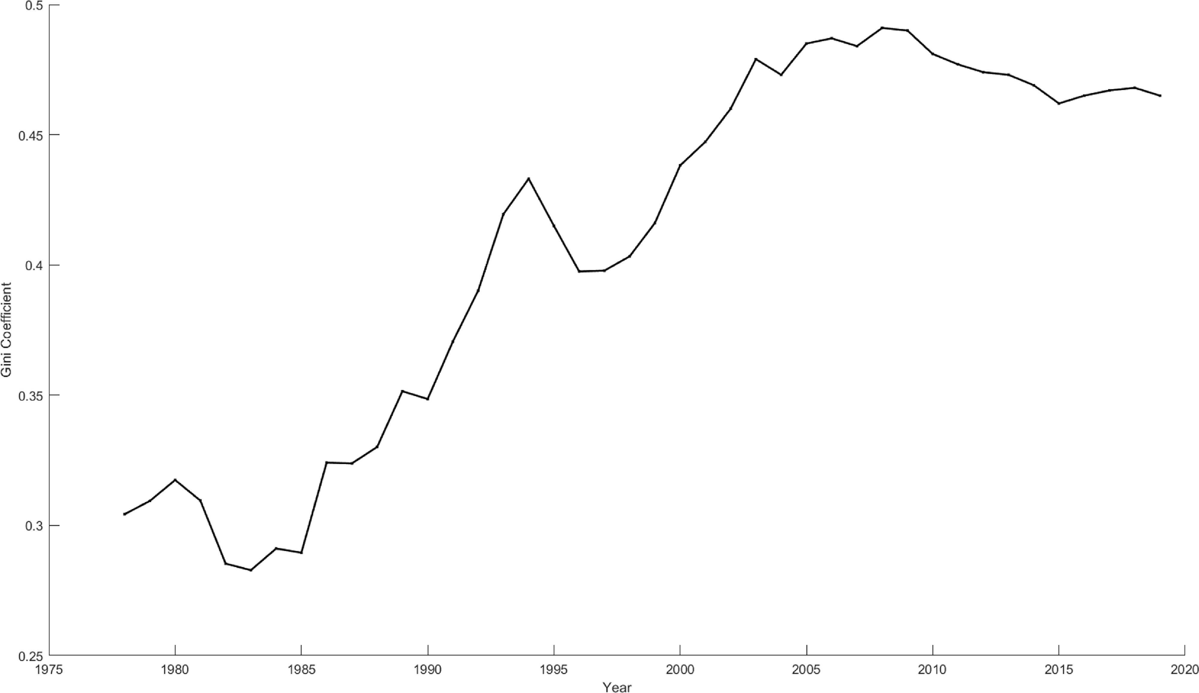
Income inequality in China experienced a significant rise from 1978 to 2008 but has witnessed a modest reduction in the last few decades.Footnote 2 The literature has identified several factors contributing to this recent decrease in income inequality, including the diffusion of technology, urban–rural migration, the returns on human capital, and trade liberalization, as highlighted by Zhang (Reference Zhang2021). Our research explores an innovative mechanism driven by gender imbalances in China, suggesting that these imbalances have shifted the patterns of assortative matching, subsequently influencing income inequality.
Marriage market matching patterns have important implications for many economic outcomes. Sorting in marriages affects the next generation’s educational attainment, human capital accumulation, income inequality, and labor force participation decisions, as widely documented in the literature by Becker (Reference Becker1974); Fernandez et al. (Reference Fernandez, Guner and Knowles2005); Greenwood et al. (Reference Greenwood, Guner, Kocharkov and Santos2014). An important determinant of marriage market outcomes is the sex ratio, i.e., the ratio of males to females in the population. Studies such as Abramitzky et al. (Reference Abramitzky, Delavande and Vasconcelos2011); Du et al. (Reference Du, Wang and Zhang2015); Yao et al. (Reference Yao, Zhang and Li2023) find that sex imbalance influences the relative status (bargaining power, parent’s wealth gap, personal income gap, etc.) of men and women in the marriage market, which has changed the degree of assortative mating.
In this study, we begin with an empirical analysis of how the sex ratio in the marriage market affects assortative matching and household income inequality. Using household surveys, regional data, and population census information, we find that a higher sex ratio is associated with a lower degree of assortative marriage, measured by educational correlation, and with lower household income inequality. To address potential endogeneity concerns, we employ an instrumental-variable strategy. The instrument is both strong and valid, and the estimated coefficients on the sex ratio remain negative and statistically significant, consistent with the OLS results. These findings strengthen the credibility of our causal interpretation.
Inspired by empirical observations, we develop a heterogeneous-agent general equilibrium model to explain the findings and explore the underlying mechanisms. Our model, inspired by the approach of Fernandez et al. (Reference Fernandez, Guner and Knowles2005), employs a two-stage matching framework that aims to capture the features of the marriage market characterized by an imbalance in the number of men and women. Our main modeling contribution relative to Fernandez et al. (Reference Fernandez, Guner and Knowles2005) is the introduction of an exogenous and variable sex ratio in the marriage market, which enables us to analyze how demographic imbalances shape assortative matching and household income inequality—an extension beyond their original framework. Within this model, individuals can be classified as either skilled or unskilled. Before entering the marriage market, each person decides on their level of education, taking into consideration the anticipated returns from matching outcomes in the marriage market. Upon completion of their education, individuals enter the marriage market where they undergo one or two rounds of matching. In this market, an individual randomly encounters a member of the opposite sex. They observe the type of skill of each other, which perfectly predicts the future income of an individual. In addition, a matched couple draws a match-specific quality (“love”) shock, and jointly decide whether to form a married couple or to remain single.
The quantitative results reveal that a higher sex ratio in the marriage market lowers assortative matching and reduces household income inequality. The mechanism operates through men’s declining reservation match quality: as the surplus of men rises, they become less selective, leading to a greater share of random matches formed in the first stage. This shift weakens positive assortative mating and, in turn, diminishes household income inequality. The negative relationship between the sex ratio and inequality is robust across different measures of income dispersion. Lastly, we explore gender-specific responses in educational attainment decisions when they expect marriage competition among men to be more intensive. The model simulations indicate that an increasing sex ratio prompts both men and women to enhance their educational investments, with men investing more significantly than women.
1.2 Related literature
This study is closely related to two strands of the literature. Firstly, it relates to the research that investigates the interaction between household assortative matching and income inequality. Becker (Reference Becker1973, Reference Becker1974) highlighted that males often marry females with similar socioeconomic backgrounds and that assortative matching is positively associated with household income inequality. Greenwood et al. (Reference Greenwood, Guner, Kocharkov and Santos2014, Reference Greenwood, Guner, Kocharkov and Santos2016, Reference Greenwood, Guner and Vandenbroucke2017) use several waves of US census data to analyze the trend of positive assortative mating. They found that there is a rise in the positive assortative mating in the US between 1960 and 2005, and that positive assortative mating contributed to the increase of income inequality across households. Fernandez et al. (Reference Fernandez, Guner and Knowles2005) reached a similar conclusion, using data from 33 countries to show a positive correlation between assortative matching and inequality. Their developed structural model further supports this finding. Fernández and Rogerson (Reference Fernández and Rogerson2001) created a dynamic model of intergenerational education acquisition and marital sorting, illustrating that increased sorting significantly elevates income inequality. Eika et al. (Reference Eika, Mogstad and Zafar2019) analyzed data from Denmark, Germany, Norway, the UK, and the US, documenting the extent of educational assortative matching and its contribution to household income inequality in each country. However, they found that variations in the degree of assortative matching have a weak influence on the time trends of household income inequality.
Secondly, our study relates to the research on the impact of sex ratio imbalances on economic outcomes, such as education investment, household savings rates, housing prices, and crime rates. Bhaskar and Hopkins (Reference Bhaskar and Hopkins2016) theoretically suggested that an excess of males in the marriage market leads to parents over-investing in sons while under-investing in daughters. Abramitzky et al. (Reference Abramitzky, Delavande and Vasconcelos2011); Angrist (Reference Angrist2002) have shown that declining sex ratios lead to males marrying up in the social hierarchy in the United States and France, respectively. Lafortune (Reference Lafortune2013) empirically showed that a sex imbalance enhances male premarital investment in education. Wei and Zhang (Reference Wei and Zhang2011); Wei et al. (Reference Wei, Zhang and Liu2017) found that the increasing sex ratio in China prompted families with sons to save more and invest in more expensive housing, where the savings and family housing value are used to indicate male’s attractiveness in the marriage market. Edlund et al. (Reference Edlund, Li, Yi and Zhang2013) discovered a positive correlation between rising sex ratios and increasing crime rates in China. Du et al. (Reference Du, Wang and Zhang2015) observed that the gender imbalance in China has resulted in females marrying up in terms of income disparity, and parental wealth gaps. Yao et al. (Reference Yao, Zhang and Li2023) found that when females are scarce in the marriage market, males tend to marry women from lower social classes, i.e., less educated or originating from rural regions.
We contribute to the academic literature in three distinct ways. First and foremost, we enrich the existing literature on the impact of sex imbalances on economic outcomes by concentrating on whether and how gender imbalances affect household income inequality. We focus on how competition within the marriage market leads to a decrease in assortative mating, subsequently affecting household income inequality. Second, after using both aggregate and household-level data to reveal the negative association between sex imbalance and household income inequality, we offer a structural interpretation of how the sex ratio in the marriage market affects household income inequality. Our findings reveal that an elevated sex ratio in the marriage market is inversely related to the level of assortative matching, thereby reducing household income inequality. Moreover, our analysis shows that as the sex ratio increases, men become less selective compared to women. Lastly, we incorporate the endogenization of educational choices in the context of gender imbalance before entering the marriage market. This approach enables us to examine the effects of marriage market competition on educational attainment in China, revealing that an increased sex ratio prompts both genders to enhance their educational investments.
The rest of the paper is organized as follows. Section 2 provides empirical evidence. Section 3 constructs a model to rationalize the empirical findings and explore the underlying mechanisms at play. Section 4 presents the quantitative results. Section 5 concludes.
2. Empirical evidence
2.1 Data and sample
The data for this study are sourced primarily from the Chinese Household Income Projects (hereafter CHIPs), the Chinese Population Census, and the China City Statistical Yearbook. We utilize data from four CHIPs waves (2002, 2007, 2013, 2018) to gather household-level information. For each wave, the CHIPs datasets include both urban and rural samples, and we utilize data from both to compile comprehensive household-level information. We pool these 4 waves of CHIPs to form the data sample that will be used in reduced-form analysis.
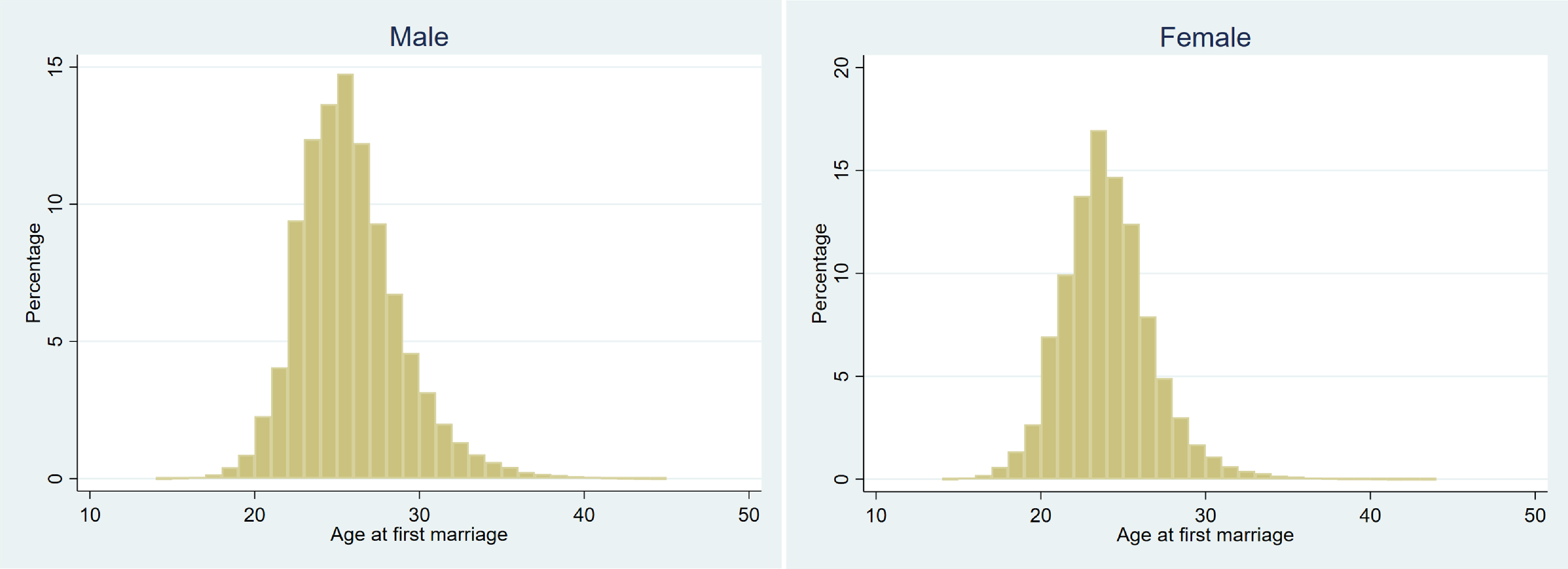
For cleaning household-level data, we limit the age range for husbands and wives to 20–35 years,Footnote 3 focusing on first marriages. The rationale for concentrating on this specific age bracket and first marriages is twofold: Firstly, the majority of Chinese couples enter into their first marriage within the age range of 20–35, as shown in Figure 1. This figure presents the age distribution of first marriages for men and women in China, highlighting that most occur between the ages of 20 and 35. Also, the legal marriage age in China is set at 22 for men and 20 for women. Secondly, examining “young marriages” provides a clearer picture of how the sex ratio in the marriage market influences matching outcomes. This is because marriage decisions for older individuals may be affected by various factors such as children, health conditions, and housing.
Age at first marriage in China.
Note: We use 1% survey data (individual level) of 2005 China’s population census to plot the age distribution for men and women.

We measure educational correlation, household income inequality, and the sex ratio in the marriage market at the prefecture level, a regional division in China akin to a city. Educational correlation is calculated from the education levels of husbands and wives in the CHIPs survey. The dataset distinguishes nine education categories,Footnote 4 and for each prefecture, we use all couples in the 20–35 age cohort to compute the correlation coefficient between spouses’ education levels. This coefficient serves as our measure of assortative marriage.
Household income is calculated as the combined job incomes of both the husband and wife. We then assess income inequality at the prefecture-level using these aggregated household incomes. The sex ratio (
 $SR_{jt}$
) is defined for each prefecture
 $j$
and wave
 $t$
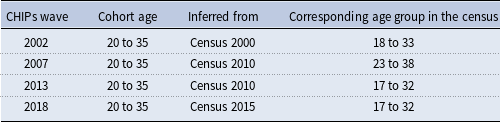
. Analyzing data at the prefectural level allows us to capture a more diverse range of sex ratio variations. This heterogeneity is depicted in Figure 2, where we illustrate the sex ratio for the 20 to 35 age cohort at the prefectural level, highlighting regional differences across China. As detailed in Wei et al. (Reference Wei, Zhang and Liu2017), due to policy constraints on internal migration and barriers related to language and culture, marriages in China are predominantly local. This suggests that the sex ratio of male to female residents, as reported in the population census, sufficiently captures the intensity of local marriage market competition. For different waves of CHIPs data, we deduce the corresponding sex ratio from various waves of the population census. Table 1 provides detailed insights into how we determine the sex ratio in the marriage market.
Cohort age selection

Note: The 2000, 2010, and 2015 censuses provide population data on males and females across various age groups (such as 5–9, 10–14, etc.).
Sex ratio for the 20 to 35 age cohort across prefectures.
Note: The darker the color, the higher the sex ratio. We employ data from the 2010 census to map out the sex ratio for the 20 to 35 age cohort at the prefecture level. The 2010 census provides data on the number of male and female residents in each county, categorized by various age groups (e.g., ages 5–9, 10–14, etc.). We aggregate these figures to the prefecture-level to calculate the sex ratio.

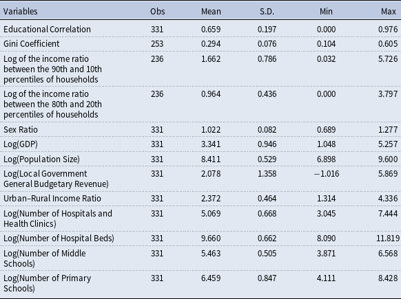
The summary statistics for the key variables are reported in Table 2. The mean educational correlation is 0.659, indicating a generally positive pattern of assortative marriage among couples in China. The Gini coefficient exhibits significant regional variation, with an average value of 0.294 and a standard deviation of 0.076. Its range extends from a minimum of 0.104 to a maximum of 0.605, indicating substantial heterogeneity in income inequality between regions. Similar patterns are observed in the analysis of two other income inequality measures: the logarithm of the income ratio between the 80th and 20th percentiles, and the logarithm of the income ratio between the 90th and 10th percentiles of households, both of which underscore the high regional variability of income inequality. Examining the sex ratio at the prefecture level, we find a standard deviation of 0.082, with the minimum and maximum values being 0.689 and 1.277, respectively, further highlighting its heterogeneity.
Summary statistics

Note: All variables are measured at the prefecture level. The Gini coefficient and the two other income inequality measures are computed by the authors using household income information from four waves of CHIPs data. The sex ratio is derived from the China Population Censuses of 2000, 2010, and 2015. All other control variables are obtained from the China City Statistical Yearbook.
2.2 Sex ratio, assortative marriage, and household income inequality
In this section, we empirically investigate how the sex ratio in the marriage market affects the degree of household assortative marriage and income inequality. Our hypothesis is that the link between the sex ratio in the marriage market and income inequality consists of two parts. First, the gender imbalance in the marriage market influences marital matching outcomes. Du et al. (Reference Du, Wang and Zhang2015) and Yao et al. (Reference Yao, Zhang and Li2023) find that the scarcity of females in China lead to men marry women from a lower social class (i.e., less educated or lower income), suggesting a decrease of assortative mating. Second, the degree of assortative matching in marriage affects household income inequality, as extensively documented in the works of Eika et al. (Reference Eika, Mogstad and Zafar2019); Fernandez et al. (Reference Fernandez, Guner and Knowles2005); Greenwood et al. (Reference Greenwood, Guner, Kocharkov and Santos2014). These studies have found a positive correlation between educational assortative marriage and income inequality.
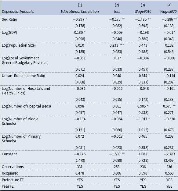
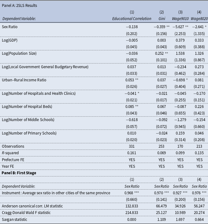
Table 3 reports the regression results, where both region and year fixed effects are controlled. To study the relationship between gender imbalances in the marriage market and the degree of assortative matching between the spouses, column (1) reports the regression results where education correlation between the spouses is used as a dependent variable. In columns (2)–(4), we study the relationship between the sex ratio and household income inequality. Household income inequality measures are represented by three metrics: the Gini coefficient (Gini), the logarithm of the income ratio between the 90th and 10th percentiles (Wage9010), and the logarithm of the income ratio between the 80th and 20th percentiles (Wage8020). In column (1), we find that the regression coefficient for the sex ratio is
 $-0.297$
, indicating that a higher sex ratio in the marriage market is associated with a lower degree of assortative matching. This finding is consistent with the existing literature. Turning to income inequality, the results in columns (2)–(4) also show negative and significant effects across all three measures, suggesting that an increase in the sex ratio reduces household income inequality. However, these OLS estimates are descriptive correlations rather than causal effects; to address potential endogeneity concerns, we turn to an instrumental-variable approach in the next section.
Sex ratio, degree of assortative matching, and household income inequality

Note: Robust standard errors in parentheses.
 $^{***}$
 $p\lt 0.01$
,
 $^{**}$
 $p\lt 0.05$
,
 $^{*}$
 $p\lt 0.1$
. We have consolidated data from four waves of CHIPs, encompassing both rural and urban samples, to gather household income information. In our analysis, we focus on couples where both the husband and wife are between 20 and 35 years old and are in their first marriage. The sex ratio in the marriage market is derived from population census data.
2.3 Instrumental variable approach
To resolve the potential endogeneity concern, we use a leave-one-out spatial instrument: the average sex ratio across other cities within the same province (excluding the target city). This variable serves as a proxy for shared regional demographic pressures, policy enforcement intensity (e.g., local implementation of the one-child policy), and cultural norms that jointly influence sex ratio imbalances across cities within a province.
This instrument satisfies the two key requirements for a valid instrumental variable: (i) Relevance: cities within the same province typically share similar demographic policies, migration patterns, birth planning norms, and economic conditions. As a result, the sex ratio in other cities is highly predictive of the target city’s own sex ratio. Our first-stage regression confirms this strong relationship, with F-statistics well above conventional thresholds. This ensures that the instrument is informative for explaining variation in the endogenous regressor (local sex ratio). (ii) Exogeneity: the leave-one-out construction ensures that the instrument does not mechanically contain information about the target city’s own outcome (i.e., educational correlation, household income inequality). Furthermore, by controlling for prefecture fixed effects and year fixed effects, we purge the influence of time-invariant local characteristics and national trends. Under these conditions, any direct effect of other cities’ sex ratios on local income inequality is highly unlikely, leaving the local sex ratio as the only plausible channel through which the instrument affects the outcome.
This approach aligns with the empirical logic of spatial and contextual instruments employed in previous studies, such as Chetty and Hendren (Reference Chetty and Hendren2018); Kleven et al. (Reference Kleven, Landais and Søgaard2019), where leave-one-out neighborhood averages are used to isolate local causal effects without contamination from the target unit’s own data.
The 2SLS estimates are reported in Table 4. Across all specifications, the coefficients on the sex ratio remain negative, consistent with the baseline regressions.Footnote 5 The effects on household income inequality are negative and statistically significant across all three measures. Moreover, the magnitudes are larger in absolute terms compared with the OLS estimates, implying that failing to account for endogeneity biases the baseline estimates toward zero. For instance, the IV coefficient for the 90/10 income ratio is −5.627, substantially larger than its OLS counterpart. This suggests that unobserved factors—such as selective migration or local shocks correlated with both sex ratios and income distribution—may have attenuated the baseline results.
The effect of sex ratio on assortative marriage and household income inequality: 2SLS estimates

Note: All regressions control for prefecture and year fixed effects. Robust standard errors clustered at the prefecture level are in parentheses. Panel B reports first-stage results and instrument diagnostics.
 $^{***}$
 $p\lt 0.01$
,
 $^{**}$
 $p\lt 0.05$
,
 $^{*}$
 $p\lt 0.1$
. The number of observations is smaller in the IV regressions because the construction of the instrument (prefecture–year average sex ratio) and the absorption of fixed effects drop prefecture–year cells with missing instruments or singleton groups. The reduction in sample size is therefore mechanical and does not reflect selective exclusion of data.
Taken together, these findings reinforce the causal interpretation of our main result: demographic imbalances in the marriage market systematically reduce household income inequality.
3. The model
In this section, we develop a heterogeneous-agent general equilibrium model that builds on Fernandez et al. (Reference Fernandez, Guner and Knowles2005), and use it to study the impact of the increasing sex ratio (“male abundance”) on household assortative matching and its implications for income inequality. Different from their framework, we explicitly introduce gender imbalance in the marriage market by allowing the sex ratio to be exogenously determined and varied across scenarios. This modeling innovation enables us to move beyond the balanced setting of Fernandez et al. (Reference Fernandez, Guner and Knowles2005) and directly analyze how demographic imbalances shape marriage market outcomes.
3.1 Setup
The economy is populated by individuals of two genders, men and women. Both men and women can be either skilled, “
 $s$
”, or unskilled, “
 $u$
”. There are four types of agents: skilled men, skilled women, unskilled men, and unskilled women. Following Fernandez et al. (Reference Fernandez, Guner and Knowles2005), we employ a two-stage matching model. In the first stage, matches are formed randomly across genders, while in the second stage, unmatched individuals are paired within their education group (i.e., skilled with skilled and unskilled with unskilled).
Before entering the marriage market, each individual decides what education level to acquire: they can become skilled or unskilled. Once they have finished their education, all agents enter the marriage market, where they go through one or two rounds of matching. They observe each other’s skill type, which perfectly predicts the future income of an individual. In addition, a matched couple draws a match-specific quality (“love”) shock, and jointly decide whether to form a married couple or to remain single.
Men and women in a married couple share a common joint utility function. Each agent is assumed to derive utility from consumption and from the quality of his (her) match. The indirect utility function for a couple with match quality
 $q$
and household income
 $I$
is:
 \begin{equation} V(I,q)=U(I)+q=U[e(w_{m}^{z}+w_{f}^{z})]+q \end{equation}
where
 $U$
is a continuous and strictly increasing function of
 $I$
;
 $w_{m}^{z}$
denotes the wage of males with skill type
 $z$
(
 $z$
is either skilled “
 $s$
” or unskilled “
 $u$
”) and
 $w_{f}^{z}$
denotes the wage of females with skill type
 $z$
.
 $e$
is used to measure the consumption equivalence scale, which is a measure of the cost of living for a household given family size and demographic composition. We follow the literature and set
 $e=0.7$
in this study. Household income is:
 \begin{equation} I=\left \{\begin{array}{ll} w^{s}_{m}+w^{s}_{f}, \\ w^{s}_{m}+w^{u}_{f}, \\ w^{u}_{m}+w^{s}_{f}, \\ w^{u}_{m}+w^{u}_{f}, \\ \end{array}\right . \end{equation}
The total number of men is normalized to 1 (
 $N^m=1$
). As a result of the “male abundance,” the number of women is smaller than the number of men (
 $N^f\lt 1$
). In the model,
 $\frac {N^m}{N^f}=\frac {1}{N^f}$
denotes the sex ratio in the marriage market.
 $\psi _m$
is the share of skilled men among all men,
 $\psi _f$
is the share of skilled women among all women.
3.2 Matching
There are two rounds of matching in the marriage market. In the first round, agents meet randomly and draw a random match-specific quality
 $q$
. We assume that
 $q$
is non-negative and follows a continuous distribution, taking the possible values in the
 $[0,q_{\max }]$
interval.Footnote
6
The cumulative distribution function (CDF) of
 $q$
is
 $Q$
, with the expected value equal to
 $\mu$
. The match can be accepted by both agents (resulting in a marriage), or rejected by at least one of the agents. In the latter case, both agents go to the second round of matching.
In the second round, all remaining unmatched women are guaranteed a partner within their own education group (skilled unmarried women are matched with skilled unmarried men, while unskilled unmarried women are matched with unskilled unmarried men). A new random match quality is drawn from the same distribution
 $Q$
. Since the number of men exceeds the number of women (
 $N^m \gt N^f$
), all women will eventually be matched, but some men may remain single after the second stage. This feature ensures the consistency of the model and reflects the demographic imbalance that motivates our analysis.
Let
 $\bar {q}_{g}^{zz}$
be the cutoff match quality for an agent with gender
 $g$
and in a match type
 $zz$
, where
 $g \in \{m,f\}$
, and
 $zz \in \{ss,su,us,uu\}$
. Below this cutoff, the agent will not accept the match. Thus, the probability of agents getting married is
 $1-Q\big[\max (\bar {q}_{m}^{zz},\bar {q}_{f}^{zz})\big]$
.
In the first round, the total number of meetings is
 $N^f$
. Since
 $N^m\gt N^f$
, some men will not meet a potential partner. For example, the number of meetings between skilled male and unskilled female is:
 $N^{f}\psi _{m}(1-\psi _{f})$
.
In the second round, some part of the remaining unmarried skilled males match (and get married) with skilled females, and some part of the remaining unmarried unskilled males match (and get married) with unskilled females. Let
 $\theta _{g}^{z}$
stand for the number of unmarried agents after the first round of the match with gender
 $g$
and skill type
 $z$
. For instance, the number of unmarried unskilled males after round 1 is:
 \begin{eqnarray} \theta _{m}^{u}&=&\big(1-N^{f}\big)(1-\psi _{m})+N^{f}(1-\psi _{m})\psi _{f}Q\big[\max \big(\bar {q}^{us}_{m},\bar {q}^{us}_{f}\big)\big]\nonumber\\&&+N^{f}(1-\psi _{m})\big(1-\psi _{f}\big)Q\big[\max \big(\bar {q}^{uu}_{m},\bar {q}^{uu}_{f}\big)\big] \end{eqnarray}
There is a trade-off between accepting the first round of matching and rejecting it, in which case the agent goes to the second round of matching. In particular, a skilled male who meets an unskilled female in the first round and draws a high match quality will encounter a trade-off between forming a lower-income household with high match quality, or rejecting this match and forming a higher-income household with a skilled female in the second round but with an expected match quality that is
 $\mu$
.
3.3 Equilibrium
Given
 $V(I,q)=U(I)+q$
, a skilled male will be indifferent between accepting a first-round match with an unskilled female and rejecting that match and entering into second round if:
 \begin{equation*}V\big(I, \bar {q}_{m}^{su}\big)=E[V(I, \mu )]\end{equation*}
where
 $\bar {q}_{m}^{su}$
denotes the reservation match quality for the skilled male when he meets with an unskilled female. The first character in the superscript “
 $s$
” is used to denote the male’s skill type, whereas the second character “
 $u$
” is used to denote the female’s skill type (we follow the same notations in the rest of the paper).
In the following part, we use this notation to represent the reservation match quality for each type of agent. Thus, there are eight reservation match qualities in total. The equilibrium is determined by eight match quality cutoffs in the first round. Solving for the value of
 $q$
at the equilibrium yields the reservation quality of
 $\bar {q}_{g}^{zz}$
.
In round 1, a skilled male matches with a skilled female will be indifferent if:
 \begin{equation*} U\big[e\big(w_{m}^{s}+w_{f}^{s}\big)\big]+\bar {q}^{ss}_{m}=\min \left(\frac {\theta _{f}^{s}}{\theta _{m}^{s}},1\right)\big[U\big[e\big(w_{m}^{s}+w_{f}^{s}\big)\big]+\mu \big]+\left [1-\min \left(\frac {\theta _{f}^{s}}{\theta _{m}^{s}},1\right)\right ]U\big(w_{m}^{s}\big) \end{equation*}
And if
 \begin{equation*} U\big[e\big(w_{m}^{s}+w_{f}^{s}\big)\big]+q_{\min }\gt \min \left(\frac {\theta _{f}^{s}}{\theta _{m}^{s}},1\right)\big[U\big[e\big(w_{m}^{s}+w_{f}^{s}\big)\big]+\mu \big]+\left [1-\min \left(\frac {\theta _{f}^{s}}{\theta _{m}^{s}},1\right)\right ]U\big(w_{m}^{s}\big) \end{equation*}
then all the skilled male that are matched with a skilled female will want to get married in round 1.
If
 \begin{equation*} U\big[e\big(w_{m}^{s}+w_{f}^{s}\big)\big]+q_{\max }\lt \min \left(\frac {\theta _{f}^{s}}{\theta _{m}^{s}},1\right)\left [U\big[e\big(w_{m}^{s}+w_{f}^{s}\big)\big]+\mu \right ]+\left [1-\min \left(\frac {\theta _{f}^{s}}{\theta _{m}^{s}},1\right)\right ]U(w_{m}^{s}) \end{equation*}
then no skilled male matched with a skilled female will want to get married in round 1. Where
 $q_{\max }$
,
 $q_{\min }$
represent the upper bound and lower bound of match quality.
In summary, the equilibrium is characterized by eight indifference conditions. As an illustration, consider the indifference condition for an unskilled male when paired with a skilled female; the remaining conditions are presented in Appendix B.
 \begin{equation} U\big[e\big(w_{m}^{u}+w_{f}^{s}\big)\big]+\bar {q}^{us}_{m}=\min \left(\frac {\theta _{f}^{u}}{\theta _{m}^{u}},1\right)\left [U\big[e\big(w_{m}^{u}+w_{f}^{u}\big)\big]+\mu \right ]+\left [1-\min \left(\frac {\theta _{f}^{u}}{\theta _{m}^{u}},1\right)\right ]U(w_{m}^{u}) \end{equation}
3.4 Equilibrium distribution of households
Since we have solved the reservation match quality for different types of match, we can generate the equilibrium distribution of household types. Let
 $\pi _{zz}$
denotes the number of different types of households in the population, thus we have:
The number of skilled husband with skilled wife in the population:
 \begin{equation*}\pi _{ss}=\underbrace {N^{f}\psi _{m}\psi _{f}\left (1-Q \big[ \! \max \big(\bar {q}^{ss}_{m},\bar {q}^{ss}_{f}\big)\big]\right )}_{\text{marriage at the first round}} \ \ \ \ +\underbrace {\min (\theta _{m}^{s},\theta _{f}^{s})}_{\text{marriage at the second round}}\end{equation*}
The number of skilled husband with unskilled wife in the population:
 \begin{equation*}\pi _{su}=N^{f}\psi _{m}(1-\psi _{f})\left (1-Q\big[ \! \max \big(\bar {q}^{su}_{m},\bar {q}^{su}_{f}\big)\big]\right )\end{equation*}
For other types of households in the population, we present them in Appendix B.
Note that we have:
 \begin{equation*}\pi _{ss}+\pi _{su}+\pi _{us}+\pi _{uu}=N^{f}\end{equation*}
Also have:
 \begin{equation*}\pi _{ss}+\pi _{su}+\pi _{us}+\pi _{uu}+\pi _{s}+\pi _{u}=1\end{equation*}
where the total number of marriages equals the number of females in the population.
3.5 Education correlation between husband and wife
Definition: we define the education correlation between husband and wife
 $\rho$
as:
 \begin{equation} \rho =\frac {\frac {\pi _{ss}}{N^{f}}-\frac {\pi _{ss}+\pi _{su}}{N^{f}}\frac {\pi _{ss}+\pi _{us}}{N^{f}}}{\sqrt {\left(\frac {\pi _{ss}+\pi _{su}}{N^{f}}\right)-\left(\frac {\pi _{ss}+\pi _{su}}{N^{f}}\right)^2}\sqrt {\left(\frac {\pi _{ss}+\pi _{us}}{N^{f}}\right)-\left(\frac {\pi _{ss}+\pi _{us}}{N^{f}}\right)^2}} \end{equation}
We show the detailed derivations and descriptions in Appendix B.
4. Quantitative analysis
4.1 Calibration
The model is calibrated to match the empirical evidence and reproduce quantitative properties. The utility function takes the form of:
 \begin{equation*}U(I)=log(I)\end{equation*}
We assume the match quality
 $q$
follows a continuous uniform distribution. The support of
 $q$
is
 $[0,1]$
, where the expected value is
 $\mu =0.5$
in this setting. A skilled agent is defined as someone who possesses educational qualifications beyond junior middle school, including those from senior middle school, vocational senior secondary school, polytechnic colleges, undergraduate programs, and graduate degrees.Footnote
7
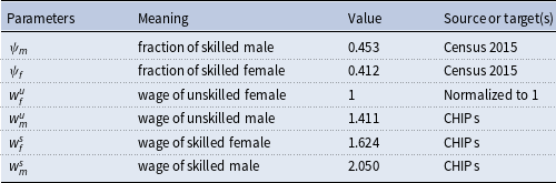
The wages for different types of agents are exogenously calibrated. We employ CHIPs 2018 data to project lifetime wages for four types of agents, as it covers the most number of provinces in China compared with other waves of CHIPs data.Footnote 8 The life cycle of an individual is divided into 5-year intervals, the age range of men is from 20 to 60, and the age range of women is from 20 to 55, the different selection is due to the mandatory retirement age in China, which is different for men and women (the restricted age is 60 for men and 55 for women). For the projections of lifetime wage of males, the interval is 20–24, 25–29, 30–34, …, 56–60. For females, it’s up to 55. The wage we used is the before-tax net labor wage, as tax may play a role in redistributing incomes. We initially compute the average wage of unskilled women in the age group of 20–24, and do so for other age groups until the group of 51–55, then use the annual discount factor of 0.96 to get the present value of unskilled women’s lifetime wages.Footnote 9 We follow the same procedures to compute the lifetime wages of skilled women, unskilled men, and skilled men. The wage of the unskilled female is normalized to 1, and we use the wage premiums to obtain those for skilled females, unskilled males, and skilled males. Where the wage premium of a skilled female is equal to the ratio of the projected lifetime wage for a skilled female over an unskilled female, the same setting applies to other types of agents.
The skilled shares of men (
 $\psi ^{m}$
) and women (
 $\psi ^{f}$
) are also calibrated to match empirical evidence. The study uses the Chinese population census 2015 to measure the fraction of skilled men and skilled women.
We vary the number of women in the model,
 $N^{f}$
, in the range from 0.81 to 0.98, which implies the sex ratio varies from 1.031 to 1.235. The detailed calibration results can be found in Table 5.
Calibrated parameters

How model fit to data

Note: We compute the mean of the education correlation using the data sample from the empirical analysis.
Assortative matching and sex ratio.

4.2 Education correlation between couples
To study the impact of gender imbalances on the degree of assortative matching, we vary the sex ratio in our model and investigate what happens to the education correlation (computed using the formula in equation (5)) in equilibrium. Using education correlation between couples as a proxy for the degree of assortative matching in marriages follows the idea of Eika et al. (Reference Eika, Mogstad and Zafar2019); Greenwood et al. (Reference Greenwood, Guner, Kocharkov and Santos2014).
As illustrated in Figure 3, the education correlation between couples is decreasing with the increase in the sex ratio. The intuition here is that the rising number of males in the marriage market makes men less likely to find a wife, thus males are less selective, which results in a decrease in assortative matching.Footnote 10 This finding is consistent with the results of other papers; Du et al. (Reference Du, Wang and Zhang2015); Yao et al. (Reference Yao, Zhang and Li2023) find that when females are scarce, males tend to marry females of a lower social class, i.e., those who are less educated, have lower personal income and come from families with lower wealth.
To check how the model fits with the data, we compare the moments of education correlation between model output and data sample. The results are reported in Table 6, we find the mean of education correlation in the model output is close to the value in the data sample, which is 0.6256 and 0.6183 respectively.
4.3 Implication for household income inequality
This section reports on how the sex ratio in the marriage market impacts household income inequality. Multiple indices are used to measure income inequality. First, we use the Gini coefficient to reveal the relationship between the sex ratio in the marriage market and household income inequality. By constructing the Lorenz curve (formulating the cumulative household share and cumulative income share), the Gini coefficient can be derived analytically, the derivations are reported in Appendix D.
Gini coefficient and sex ratio.

Sex ratio and household income inequality.

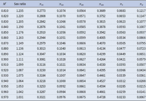
Figure 4 illustrates that in the marriage market, the sex ratio is inversely correlated with the Gini coefficient, suggesting that a higher sex ratio correlates with lower household income inequality. The underlying rationale for this pattern relates to the positive association between assortative marriage and household income inequality, a theme explored in several studies (e.g., Eika et al. (Reference Eika, Mogstad and Zafar2019); Fernandez et al. (Reference Fernandez, Guner and Knowles2005); Greenwood et al. (Reference Greenwood, Guner, Kocharkov and Santos2014)). Conversely, our prior analysis reveals that an elevated sex ratio corresponds to reduced assortative matching. This inverse relationship indicates that a higher sex ratio may lead to decreased household income inequality. Intuitively, a decline in assortative marriage suggests a reduction in the proportion of couples with similar education levels (positive assortative mating) and an increase in couples with differing education levels, as shown in Table C2. These shifts in household formation contribute to the reduction in household income inequality, reinforcing our conclusion that the sex ratio is negatively associated with household income disparity.
We also use other measures to study how the sex ratio impacts the inequality of household income. Figure 5 presents four measures of income inequality, which are the coefficient of variation, Theil L index, Theil T index, and logarithmic variance, respectively. These indices provide a more comprehensive understanding of the income distribution and its skewness. For instance, the coefficient of variation emphasizes the standard deviation of income relative to the mean, offering insights into the overall variability of household income. On the other hand, Theil’s indices, particularly the L and T variants, offer a decomposition feature that allows for a detailed analysis of inequality within and between different population subgroups. Similarly, the logarithm of variance addresses scale dependency issues by normalizing the variance, thus providing a measure of dispersion that is not influenced by the income level itself (see Cowell, Reference Cowell2011).
Our analysis, as shown in Figure 5, demonstrates that the sex ratio in the marriage market exhibits a consistent inverse relationship with these indices. Specifically, the coefficient of variation, which gauges the dispersion of income around the mean, shows a downward trend as the sex ratio increases, indicating a contraction in relative income disparities. Furthermore, the Theil indices, both L and T, show a similar downward trend with an increasing sex ratio. The Theil L index, which places greater emphasis on the lower tail of the income distribution, suggests that a higher sex ratio may contribute to raising incomes at the lower end, thereby reducing inequality. The Theil T index, more sensitive to the upper tail, implies that the top earners’ share of total income decreases as the sex ratio rises. This could be interpreted as a decline in the income advantage that typically accrues to households with high educational or occupational homogamy, as the sex ratio increases. Lastly, the logarithmic variance, which mitigates the scale dependency of variance, also shows a reduction with an elevated sex ratio. This indicates that income differences between households are becoming less pronounced, leading to a more even spread of earnings among families.
4.3.1 Quantitative comparison between the model and data
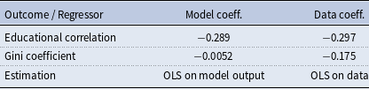
In this section, we present a quantitative comparison between the model and the empirical results. Specifically, we replicate the regressions reported in Table 3 using the simulated data from the calibrated model and contrast the resulting coefficients with those obtained from the empirical sample.
The comparison highlights two key findings (see Table 7). First, the model reproduces the relationship between sex ratios and assortative marriage well. The estimated coefficient of the sex ratio on educational correlation is −0.289, closely aligned with the empirical estimate of −0.297. This correspondence suggests that the model successfully captures the mechanism by which a male-biased marriage market increases the share of random matches, thereby weakening assortative matching.
Second, the model predicts a smaller impact of sex ratios on household income inequality than observed in the data. For the Gini coefficient, the model delivers an estimate of −0.0052, compared with an empirical coefficient of −0.175, While the direction of the effect is consistent, the magnitude is underestimated. This limitation stems from the parsimonious structure of the model, which includes only four discrete household types. Such structure flattens the Lorenz curve and may dampen the sensitivity of inequality measures to changes in household composition. We view this as a promising direction for future research: extending the framework to incorporate richer heterogeneity—such as multiple skill levels or continuous wage distributions—would allow the model to generate a more nuanced income distribution and better match the empirical magnitudes of inequality responses.
Model-implied coefficients vs. data estimates

Note: Coefficients are estimated from regressions of each outcome on the sex ratio. “Model coeff.” is based on simulated data from the calibrated model; “Data coeff.” is based on the empirical sample.
4.4 Inspecting the mechanisms
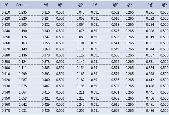
The negative effect of the sex ratio on assortative matching in our model operates through the interaction of reservation thresholds and the two-stage matching structure. When the number of men increases, competition in the marriage market intensifies. As a result, men become less selective: they lower the reservation match quality that they are willing to accept in the first round. Figure 6a illustrates this pattern across different skill pair types, showing that the reservation cutoff declines as the sex ratio rises.
Reservation match quality for men and first-stage marriage rate.

This decline in reservation thresholds has direct implications for the share of first-stage marriages. Because the first round involves random matching across education groups, a lower reservation cutoff increases the probability that men accept these random matches. As shown in Figure 6b, the first-stage marriage rate rises monotonically with the sex ratio. More marriages are therefore concluded in the random stage, reducing the role of the second-stage within-group (assortative) matching.
The shift toward a greater share of random matches has important distributional consequences. Since random matches weaken the positive correlation between spouses’ education levels, the overall degree of assortative matching falls. With less assortative sorting by education, income differences across households narrow, leading to lower household income inequality in equilibrium.
4.5 Robustness check: alternative matching function
To examine the robustness of our results, we consider a more general specification of the matching function. Following Den Haan et al. (Reference Den Haan, Ramey and Watson2000), we allow the meeting probabilities on both sides of the market to vary with the sex ratio rather than assuming that each woman is guaranteed to meet a partner in the first stage. The general matching function is defined as:
 \begin{equation} M(X,Y) = \frac {XY}{\Big(X^{\tfrac {1}{\omega }}+Y^{\tfrac {1}{\omega }}\Big)^{\omega }} \end{equation}
where
 $M$
denotes the number of matches between two groups,
 $X$
and
 $Y$
represent the number of agents on each side of the market (men and women), and
 $\omega \gt 0$
is the elasticity of substitution between them. In our context, the formulation becomes:
 \begin{equation} M(N^{m},N^{f}) = \frac {N^{m}N^{f}}{\bigg ((N^{m})^{\tfrac {1}{\omega }}+(N^{f})^{\tfrac {1}{\omega }}\bigg)^{\omega }} \end{equation}
Our baseline assumption corresponds to the limiting case as
 $\omega \to 0$
, in which each woman is guaranteed to meet a man in the first stage. By allowing finite values of
 $\omega$
, this specification relaxes the baseline assumption and makes women’s meeting probabilities responsive to demographic imbalances.
Quantitative experiments under different values of
 $\omega$
show that our main results remain robust. Although a higher probability of meeting a partner allows women to be more selective, the overall pattern persists: a higher sex ratio reduces assortative matching and, in turn, lowers household income inequality. This confirms that our key insights are not an artifact of the baseline assumption but hold under a broader class of matching technologies. Detailed derivations and numerical results are reported in Appendix E.
Decision tree for the male who wants to become skilled.

4.6 Education decision
In previous sections, the skilled labor shares for both males and females were exogenously calibrated. This section, however, explores how agents choose their education levels. Specifically, it aims to conduct a counterfactual experiment examining the choices of males and females in education, considering their expectations of intensified competition in the marriage market among men and reduced competition among women due to changing sex ratios. To investigate this, we model agents making educational investment decisions before entering the marriage market. We denote the period when agents decide on their education as
 $t$
and the period when they enter the marriage market competition as
 $t+1$
.
In period
 $t$
, agents form expectations regarding the utility gains from matches occurring in the following period,
 $t+1$
. These expectations guide their decision to pursue either a skilled or unskilled path. The process of deciding to become a skilled or unskilled agent involves various scenarios, and we have delineated the expected value function for clarity. Initially, we elucidate the expected payoff for a skilled male using a decision tree diagram, followed by a formal expression of the expected payoff equation. The expected payoff equations for the other three agent types are detailed in Appendix F, along with corresponding decision tree diagrams. These decision trees carefully map out each step’s potential outcomes, allowing for the calculation of the associated expected utility.
Figure 7 presents a decision tree for a man who wants to become skilled. In the first round of matching, he encounters one of three possible outcomes: meeting a skilled female (
 $f_{s}$
), an unskilled female (
 $f_{u}$
), or no one at all (“-”), a scenario that arises when the number of males (
 $N^{m}=1$
) exceeds the number of females (
 $N^{f}$
). If he meets a skilled female (
 $f_{s}$
), he may either agree to marry (“Yes”) or decline the match (“No”), moving to the second round. In the second round, he can either successfully pair with a skilled female and marry or remain single. Similarly, if he meets an unskilled female (
 $f_{u}$
), he faces the choice to either form a household with her (“Yes”) or refuse (“No”) and proceed to the second round. Here, he may marry a skilled female (
 $f_{s}$
) or end up single (“Single”). If he meets no one in the first round (“-”), he directly advances to the second round, where he either finds a skilled female to marry or remains single (“Single”).
The expected utility of being a skilled male given the fraction of
 $\psi ^{f}_{t+1}$
skilled female is:
 \begin{align} \mathrm E_{t}{V_{m}^{s}} & \big(\psi _{t+1}^{m},\psi _{t+1}^{f}\big) = \psi _{t+1}^{f}{N^{f}_{t+1}} \left \{ \int _{\max (\bar {q}_{m}^{ss},\bar {q}_{f}^{ss})}^{q_{\max }} \left[U\big(e\big[w_{m}^{s}+w_{f}^{s}\big]\big)+q_{m}^{ss}\right]dq\right . \nonumber\\[8pt] & \quad \left .\ +Q\big[ \! \max \big(\bar {q}_{m}^{ss},\bar {q}_{f}^{ss}\big)\big] \min\! \left(\frac {\theta _{f}^{s}\big(\psi _{t+1}^{m},\psi _{t+1}^{f}\big)}{\theta _{m}^{s}\big(\psi _{t+1}^{m},\psi _{t+1}^{f}\big)},1\right)\!\int _{0}^{q_{\max }}\big[U\big(e\big[w_{m}^{s}+w_{f}^{s}\big]\big)+q_{m}^{ss} \big]dq\right .\nonumber\\[8pt] &\quad\left . \ +Q\big[ \! \max \big(\bar {q}_{m}^{ss},\bar {q}_{f}^{ss}\big)\big] \left [1-\min \left(\frac {\theta _{f}^{s}\big(\psi _{t+1}^{m},\psi _{t+1}^{f}\big)}{\theta _{m}^{s}\big(\psi _{t+1}^{m},\psi _{t+1}^{f}\big)},1\right)\right ]U[w_{m}^{s}] \right \} \nonumber\\[8pt] &\quad+(1-\psi _{t+1}^{f})N^{f}_{t+1}\left \{\int _{\max (\bar {q}_{m}^{su},\bar {q}_{f}^{su})}^{q_{\max }}\left [U\big(e[w_{m}^{s}+w_{f}^{u}]\big)+q_{m}^{su}\right ]dq\right .\nonumber\\[8pt] &\quad\left .\ +Q\big[ \! \max \big(\bar {q}_{m}^{su},\bar {q}_{f}^{su}\big)\big]\min \left(\frac {\theta _{f}^{s}\big(\psi _{t+1}^{m},\psi _{t+1}^{f}\big)}{\theta _{m}^{s}\big(\psi _{t+1}^{m},\psi _{t+1}^{f}\big)},1\right)\int _{0}^{q_{\max }}\left [U\big(e\big[w_{m}^{s}+w_{f}^{s}\big]\big)+q_{m}^{ss}\right ]dq\right .\nonumber\\[8pt] &\quad\left .\ +Q\big[ \! \max \big(\bar {q}_{m}^{su},\bar {q}_{f}^{su}\big)\big]\left [1-\min \left(\frac {\theta _{f}^{s}\big(\psi _{t+1}^{m},\psi _{t+1}^{f}\big)}{\theta _{m}^{s}\big(\psi _{t+1}^{m},\psi _{t+1}^{f}\big)},1\right)\right ]U\left [w_{m}^{s}\right ]\right \}\nonumber\\[8pt] &\quad +(1-N^{f}_{t+1})\left \{\min \left(\frac {\theta _{f}^{s}\big(\psi _{t+1}^{m},\psi _{t+1}^{f}\big)}{\theta _{m}^{s}\big(\psi _{t+1}^{m},\psi _{t+1}^{f}\big)},1\right)\int _{0}^{q_{\max }} \left [U\big(e\big[w_{m}^{s}+w_{f}^{s}\big]\big)+q_{m}^{ss}\right ]dq\right .\nonumber\\[8pt] &\quad\left . \ +\left [1-\min \left(\frac {\theta _{f}^{s}\big(\psi _{t+1}^{m},\psi _{t+1}^{f}\big)}{\theta _{m}^{s}\big(\psi _{t+1}^{m},\psi _{t+1}^{f}\big)},1\right)\right ]U\left [w_{m}^{s}\right ] \right \} \end{align}
4.6.1 Education decision and sex ratio
Becoming a skilled agent requires some effort
 $\phi _{g}\ (g \in \{male, female\})$
, which is
 $\in [0,+\infty )$
, the effort is i.i.d. for all men and women, with the CDF of
 $\Phi _{g}$
. An agent
 $i$
wants to become skilled if:
 \begin{equation} \mathrm EV^{s}_{i}-\mathrm EV^{u}_{i}\geq \phi _{i} \end{equation}
Where
 $\mathrm EV^{s}_{i}$
is the expected payoff of becoming skilled for agent
 $i$
. The skilled-unskilled payoff difference is generated when a fraction of
 $\psi$
is skilled:
 \begin{align} \bar {\phi }\big(\psi _{t+1}^{m}\big)\equiv \mathrm E_{t}V^{s}_{m}\big(\psi _{t+1}^{m}\big)-\mathrm E_{t}V^{u}_{m}\big(\psi _{t+1}^{m}\big)\nonumber\\[5pt] \bar {\phi }\big(\psi _{t+1}^{f}\big)\equiv \mathrm E_{t}V^{s}_{f}\big(\psi _{t+1}^{f}\big)-\mathrm E_{t}V^{u}_{f}\big(\psi _{t+1}^{f}\big) \end{align}
For any individual
 $i$
: when
 $\phi _{i} \leq \bar {\phi }$
(the effort that has to be devoted to becoming a skilled individual is smaller or equal to the reservation effort
 $\bar {\phi }$
, an agent want to become skilled).
Without considering the education costs, agents can borrow freely, and contingent on their efforts, the young agent will make the same decision irrespective of their family wealth type (family provides the funding for education). This implies that in equilibrium: a fraction
 $\Phi (\bar {\phi }_{g})$
of individuals would become skilled, then the equilibrium distribution of education fraction for two genders are:
 \begin{align} \psi _{t+1}^{m} & =\Phi \big(\bar {\phi }_{m}\big)\nonumber \\[5pt] \psi _{t+1}^{f} & =\Phi \big(\bar {\phi }_{f}\big) \end{align}
Thus:
 \begin{align} \bar {\phi }\big(\Phi \big(\bar {\phi }_{m}\big)\big) & = \mathrm E_{t}V^{s}_{m}\big(\Phi \big(\bar {\phi }_{m}\big)\big)-\mathrm E_{t}V^{u}_{m}\big(\Phi \big(\bar {\phi }_{m}\big)\big)\nonumber\\[6pt] \bar {\phi }\big(\Phi \big(\bar {\phi }_{f}\big)\big) & = \mathrm E_{t}V^{s}_{f}\big(\Phi \big(\bar {\phi }_{f}\big)\big)-\mathrm E_{t}V^{u}_{f}\big(\Phi \big(\bar {\phi }_{f}\big)\big) \end{align}
We firstly assume that
 $\phi _{g}$
is a uniform distribution for both male and female, which is
 $\in [0,1]$
. Under this assumption, we have:
 \begin{align} \psi _{t+1}^{m} & = \mathrm E_{t}V^{s}_{m}\big(\psi _{t+1}^{m}\big)-\mathrm E_{t}V^{u}_{m}\big(\psi _{t+1}^{m}\big)\nonumber\\[6pt]\psi _{t+1}^{f} & = \mathrm E_{t}V^{s}_{f}\big(\psi _{t+1}^{f}\big)-\mathrm E_{t}V^{u}_{f}\big(\psi _{t+1}^{f}\big) \end{align}
Education decision and sex ratio.
Note: The results presented in the left-hand figure are derived from model outputs, while those on the right-hand side are based on four waves of population census data (census 2000, 2005, 2010, 2015). We measure the fraction of skilled men and women respectively, by restricting cohorts’ age between 20 to 35.

After integrating both sides of equation (10) and evaluating it on the whole range of
 $\phi$
(that is
 $\in [0,1]$
), we can get equation (13). After solving it, we generate the results plotted in the Figure 8a. In our matching model, agents of each gender make a binary decision regarding their education level, opting to be skilled or unskilled. This choice leads to an equilibrium distribution in the proportion of skilled agents within the population.
As illustrated in Figure 8a, we find that both men and women increasingly become skilled as the sex ratio in the marriage market increases, where the trend of men is above the trend of women, suggesting that men spend more effort in becoming skilled compared with women. Additionally, when we examine the results of the model alongside the data trends shown in Figure 8b, we observe an upward trajectory in the proportion of skilled men and women over time. This pattern suggests that our model offers insight into the increasing levels of human capital in China, indicating that the increase in male abundance induces higher human capital.
The reasons behind the trend of both men and women becoming more skilled as the sex ratio increases are as follows. For men, firstly, being skilled typically means higher earnings, which can boost their appeal in the increasingly competitive marriage market. Second, when examining the data in Table C1, we see that the probabilities of an unskilled man (
 $\pi _{u}$
) and a skilled man (
 $\pi _{s}$
) of remaining single rise with an increasing sex ratio. However, the likelihood of being single is higher for unskilled men (
 $\pi _{u}\lt \pi _{s}$
), suggesting that it’s riskier for them to find a partner. Additionally, should an unskilled man marry, he is more likely to marry an unskilled woman, as indicated by the higher values of (
 $\pi _{uu}$
) in comparison to other household types, leading to a lower utility gain in forming a household. These factors motivate men to become skilled.
For women, firstly, choosing to remain unskilled means they are more likely to marry an unskilled husband (as
 $\pi _{uu}\lt \pi _{su}$
), which generally offers less benefit. Secondly, if a woman becomes skilled, she is more likely to marry a skilled husband than an unskilled one (as
 $\pi _{ss}\gt \pi _{us}$
). Third, as the sex ratio in the marriage market increases, even though an unskilled woman’s chances of marrying a skilled husband increase, the likelihood of forming a household with skilled men is still lower than marrying an unskilled husband (as
 $\pi _{uu}\gt \pi _{su}$
). Therefore, women are more inclined to become skilled.
This finding offers a potential explanation for the observed increase in education levels in China. Analysis of census data suggests that a growing surplus of men is associated with higher educational attainment for both men and women. In addition, we enrich the literature that has studied the interconnection between premarital investment in education and marriage market competition. Lafortune (Reference Lafortune2013) finds that males increased their human capital investment when faced with an increase in the sex ratio. Bhaskar and Hopkins (Reference Bhaskar and Hopkins2016) indicate that if there is an unbalanced sex ratio, the abundant sex invests more, while the scarcer one invests less. Additionally, Bhaskar et al. (Reference Bhaskar, Li and Yi2023) illustrate that parents of boys invest less in education in regions with a more male-biased sex ratio but they invest more in housing. Our findings enrich these studies, showing that in response to an increasing surplus of males, both men and women enhance their educational investments. Notably, men’s investments in education are more pronounced compared to those of women.
5. Conclusion
The increasing gender imbalance in China has gained significant attention from economists. In this study, we investigate whether and how gender imbalance affects household income inequality. Our research suggests that growing gender imbalance may lead to a reduction in assortative mating among Chinese couples, thereby contributing to a decrease in household income inequality within the country. We first present empirical evidence to assess the influence of the sex ratio in the marriage market on household income inequality. Then, we construct a structural model to elucidate the empirical observations and investigate the underlying mechanisms.
Drawing from empirical evidence, we observe a negative correlation between the sex ratio in the marriage market and household income inequality. Specifically, an increase in the sex ratio is linked to a reduction in household income inequality. To deepen our analysis, Section 3 introduces a structural interpretation, in which we use a model to inspect the dynamics of the marriage market and matching outcomes in China.
Theoretically, the results from the model indicate that men become less selective in the marriage market when the male abundance in the marriage market increases. This results in a decrease of assortative matching. This finding is consistent with the literature’s conclusion that men tend to marry women from a lower social class in the presence of male abundance. Furthermore, our results consistently show that a rise in the sex ratio is related to a decline in household income inequality, a relationship that is robust across different measures of income inequality. Lastly, we incorporate the endogenization of individuals’ educational choices in the context of gender imbalance before they enter into the marriage market. This approach allows us to examine the impact of marriage market competition on educational attainment in China. Our results show that an elevated sex ratio leads to increased educational investments by both men and women, with men investing more significantly than women.
While our analysis focuses on China due to its unique demographic history—including the one-child policy and strong son preference—we believe that the mechanisms uncovered in our study may be applicable to other societies with significant gender imbalances. For example, countries such as India and parts of the Middle East have also experienced persistently high male-to-female sex ratios, which could lead to similar patterns of marriage market competition and its implications for household-level outcomes. Nevertheless, cultural norms and institutional settings may shape how these dynamics manifest, and the magnitude of the effects may differ across contexts. Future research could explore the extent to which our findings generalize beyond China by applying similar structural approaches to other settings.
Our analysis yields several policy relevant insights. First, the evidence suggests that male-biased sex ratios increase marriage market competition among men, which in turn encourages higher educational investment, particularly among men in affected regions. Second, higher sex ratios tend to reduce assortative matching, thereby contributing to lower household income inequality. At the same time, a persistent imbalance may leave a larger share of men unmarried, raising potential social and economic challenges. Policymakers may therefore need to complement the observed inequality-reducing effects with targeted interventions aimed at supporting unmarried and disadvantaged individuals in regions facing sustained gender imbalances.
Acknowledgments
We would like to thank two anonymous referees and an associate editor for their comments. Their feedback has greatly helped improve this paper. We also thank the comments from Alessandro Mennuni, Sekyu Choi, Michael Hatcher, Héctor Calvo Pardo, and other comments at the annual conference of the Chinese Economists Society 2023. Specifically, we thank Dr. Yuankun Li’s help.
Appendix A. Sex ratio at birth and Gini coefficient in China
Sex ratio at birth in China.
Note: We utilize data from multiple waves of the Chinese population census (1982, 1985,…2015) to calculate the sex ratio at birth in China. Each population census provides data on the number of residents in both rural and urban areas across various age groups. We utilize this information to deduce the sex ratio at birth for different years.

Gini coefficient in China.
Note: The Gini coefficient data are sourced from the National Bureau of Statistics.

Figure A1 displays the trend of the sex ratio at birth in China, revealing a significant increase following the introduction of the one child policy (OCP) in 1979. The connection between the one child policy and the sex ratio has been thoroughly examined by researchers such as Ebenstein (Reference Ebenstein2010, Reference Ebenstein2011); Zhang (Reference Zhang2017), who emphasize that a preference for sons led to the selective abortion of female fetuses, facilitated by advancements in biotechnology, as a consequence of the OCP. This policy skewed the sex ratio, with a more pronounced distortion in rural areas due to a stronger preference for sons. Notably, from 1990 onwards, the sex ratio at birth in China has risen markedly, indicating that two decades later, the marriage market experienced heightened competition among men.
Figure A2 shows the evolution of the Gini coefficient in China, revealing an upward trend in income inequality beginning in 1978, followed by a modest decline in recent years. For a detailed exploration of the changes in income inequality in China, Zhang (Reference Zhang2021) provides an extensive survey.
Appendix B. The remaining part of the model
We illustrate the remaining part of the model in this section.
The number of meetings between individuals of different skill types that take place in the first round is:
 \begin{equation} \begin{array}{ll} N^{f}\psi _{m}\psi _{f}: & \text{the number of meetings between skilled male and skilled female} \\ N^{f}\psi _{m}(1-\psi _{f}): & \text{the number of meetings between skilled male and unskilled female} \\ N^{f}(1-\psi _{m})\psi _{f}: & \text{the number of meetings between unskilled male and skilled female}\\ N^{f}(1-\psi _{m})(1-\psi _{f}): & \text{the number of meetings between unskilled male and unskilled female} \end{array} \end{equation}
The number of unmarried individuals after the first round of matching:
 \begin{align} \begin{array}{l} \theta _{m}^{s}=(1-N^{f})\psi _{m}+N^{f}\psi _{m}\psi _{f}Q\big [ \! \max \big(\bar {q}^{ss}_{m},\bar {q}^{ss}_{f}\big)\big ]+N^{f}\psi _{m}(1-\psi _{f})Q\big [ \! \max \big(\bar {q}^{su}_{m},\bar {q}^{su}_{f}\big)\big ] \\[5pt] \text{the number of unmarried skilled males after round 1} \\[5pt] \theta _{m}^{u}=(1-N^{f})(1-\psi _{m})+N^{f}(1-\psi _{m})\psi _{f}Q\big [ \! \max \big(\bar {q}^{us}_{m},\bar {q}^{us}_{f}\big)\big ]\\[5pt] \qquad +N^{f}(1-\psi _{m})(1-\psi _{f})Q\big [ \! \max \big(\bar {q}^{uu}_{m},\bar {q}^{uu}_{f}\big)\big ]\\[5pt] \text{the number of unmarried unskilled males after round 1} \\[5pt] \theta _{f}^{s}=N^{f}\psi _{m}\psi _{f}Q\big [ \! \max \big(\bar {q}^{ss}_{m},\bar {q}^{ss}_{f}\big)\big ]+N^{f}(1-\psi _{m})\psi _{f}Q\big [ \! \max \big(\bar {q}^{us}_{m},\bar {q}^{us}_{f}\big)\big ]\\[5pt] \text{the number of unmarried skilled females after round 1}\\[5pt] \theta _{f}^{u}=N^{f}\psi _{m}(1-\psi _{f})Q\big [ \! \max \big(\bar {q}^{su}_{m},\bar {q}^{su}_{f}\big)\big ]+N^{f}(1-\psi _{m})(1-\psi _{f})Q\big [ \! \max \big(\bar {q}^{uu}_{m},\bar {q}^{uu}_{f}\big)\big ]\\[5pt] \text{the number of unmarried unskilled females after round 1} \end{array} \end{align}
B.1. The full equilibrium conditions in the model
The indifference condition for a skilled male matched with a skilled female:
 \begin{equation*}U\big[e\big(w_{m}^{s}+w_{f}^{s}\big)\big]+\bar {q}^{ss}_{m}=\min \left(\frac {\theta _{f}^{s}}{\theta _{m}^{s}},1\right)\left [U\big[e\big(w_{m}^{s}+w_{f}^{s}\big)\big]+\mu \right ]+\left [1-\min \left(\frac {\theta _{f}^{s}}{\theta _{m}^{s}},1\right)\right ]U(w_{m}^{s})\end{equation*}
The indifference condition for a skilled female matched with a skilled male:
 \begin{equation*}U\big[e\big(w_{m}^{s}+w_{f}^{s}\big)\big]+\bar {q}^{ss}_{f}=\min \left(\frac {\theta _{m}^{s}}{\theta _{f}^{s}},1\right)\left [U\big[e\big(w_{m}^{s}+w_{f}^{s}\big)\big]+\mu \right ]+\left [1-\min \left(\frac {\theta _{m}^{s}}{\theta _{f}^{s}},1\right)\right ]U(w_{f}^{s})\end{equation*}
The indifference condition for an unskilled male matched with a skilled female:
 \begin{equation*}U\big[e\big(w_{m}^{u}+w_{f}^{s}\big)\big]+\bar {q}^{us}_{m}=\min \left(\frac {\theta _{f}^{u}}{\theta _{m}^{u}},1\right)\left [U\big[e\big(w_{m}^{u}+w_{f}^{u}\big)\big]+\mu \right ]+\left [1-\min \left(\frac {\theta _{f}^{u}}{\theta _{m}^{u}},1\right)\right ]U(w_{m}^{u})\end{equation*}
The indifference condition for a skilled female matched with an unskilled male:
 \begin{equation*}U\big[e\big(w_{m}^{u}+w_{f}^{s}\big)\big]+\bar {q}^{us}_{f}=\min \left(\frac {\theta _{m}^{s}}{\theta _{f}^{s}},1\right)\left [U\big[e\big(w_{m}^{s}+w_{f}^{s}\big)\big]+\mu \right ]+\left [1-\min \left(\frac {\theta _{m}^{s}}{\theta _{f}^{s}},1\right)\right ]U(w_{f}^{s})\end{equation*}
The indifference condition for a skilled male matched with an unskilled female:
 \begin{equation*}U\big[e\big(w_{m}^{s}+w_{f}^{u}\big)\big]+\bar {q}^{su}_{m}=\min \left(\frac {\theta _{f}^{s}}{\theta _{m}^{s}},1\right)\left [U\big[e\big(w_{m}^{s}+w_{f}^{s}\big)\big]+\mu \right ]+\left [1-\min \left(\frac {\theta _{f}^{s}}{\theta _{m}^{s}},1\right)\right ]U(w_{m}^{s})\end{equation*}
The indifference condition for an unskilled female matched with a skilled male:
 \begin{equation*}U\big[e\big(w_{m}^{s}+w_{f}^{u}\big)\big]+\bar {q}^{su}_{f}=\min \left(\frac {\theta _{m}^{u}}{\theta _{f}^{u}},1\right)\left [U\big[e\big(w_{m}^{u}+w_{f}^{u}\big)\big]+\mu \right ]+\left [1-\min \left(\frac {\theta _{m}^{u}}{\theta _{f}^{u}},1\right)\right ]U(w_{f}^{u})\end{equation*}
The indifference condition for an unskilled male matched with an unskilled female:
 \begin{equation*}U\big[e\big(w_{m}^{u}+w_{f}^{u}\big)\big]+\bar {q}^{uu}_{m}=\min \left(\frac {\theta _{f}^{u}}{\theta _{m}^{u}},1\right)\left [U\big[e\big(w_{m}^{u}+w_{f}^{u}\big)\big]+\mu \right ]+\left [1-\min \left(\frac {\theta _{f}^{u}}{\theta _{m}^{u}},1\right)\right ]U(w_{m}^{u})\end{equation*}
The indifference condition for an unskilled female matched with an unskilled male:
 \begin{equation*}U\big[e\big(w_{m}^{u}+w_{f}^{u}\big)\big]+\bar {q}^{uu}_{f}=\min \left(\frac {\theta _{m}^{u}}{\theta _{f}^{u}},1\right)\left [U\big[e\big(w_{m}^{u}+w_{f}^{u}\big)\big]+\mu \right ]+\left [1-\min \left(\frac {\theta _{m}^{u}}{\theta _{f}^{u}},1\right)\right ]U(w_{f}^{u})\end{equation*}
B.2. The number of different types of household in the model
The number of unskilled husband with skilled wife in the population:
 \begin{equation*}\pi _{us}=N^{f}(1-\psi _{m})\psi _{f}\left (1-Q\big[ \! \max \big(\bar {q}^{us}_{m},\bar {q}^{us}_{f}\big)\big]\right )\end{equation*}
The number of unskilled husband with unskilled wife in the population:
 \begin{equation*}\pi _{uu}=N^{f}(1-\psi _{m})(1-\psi _{f})\left (1-Q\big[ \! \max \big(\bar {q}^{uu}_{m},\bar {q}^{uu}_{f}\big)\big]\right )+\min \big(\theta _{m}^{u},\theta _{f}^{u}\big)\end{equation*}
The number of unmarried skilled male after two rounds of matching in the population:
 \begin{equation*}\pi _{s}=\max \big(\theta _{m}^{s}-\theta _{f}^{s},0\big)\end{equation*}
The number of unmarried unskilled male after two rounds of matching in the population:
 \begin{equation*}\pi _{u}=\max \big(\theta _{m}^{u}-\theta _{f}^{u},0\big)\end{equation*}
B.3. Education correlation between husband and wife
Education correlation between husband and wife
 $\rho$
is been defined as:
 \begin{equation*}\rho =\frac {Cov(X,Y)}{\sqrt {Var(X)}\sqrt {Var(Y)}}=\frac {E(XY)-E(X)E(Y)}{\sqrt {E(X^2)-E(X)^2}\sqrt {E(Y^2)-E(Y)^2}}\end{equation*}
Where
 $X$
and
 $Y$
stands for events
 $\{husband\}$
and
 $\{wife\}$
respectively, let:
 \begin{equation} \begin{array}{ll} X=\left \{\begin{array}{ll} 1 & \text{husband is skilled}\\ 0 & \text{husband is unskilled} \end{array}\right . & \quad Y=\left \{\begin{array}{ll} 1 & \text{wife is skilled}\\ 0 & \text{wife is unskilled} \end{array}\right .\\ \end{array} \end{equation}
Hence, the expectations of
 $X$
and
 $Y$
are:
 \begin{equation} \begin{array}{ll} E(X)=\frac {\pi _{ss}+\pi _{su}}{N^{f}} & \quad E(Y)=\frac {\pi _{ss}+\pi _{us}}{N^{f}} \end{array} \end{equation}
And we have:
 \begin{equation} \begin{array}{ll} E(X^2)=\frac {\pi _{ss}+\pi _{su}}{N^{f}} & \quad E(Y^2)=\frac {\pi _{ss}+\pi _{us}}{N^{f}} \end{array} \end{equation}
 \begin{equation*}E(XY)=\frac {\pi _{ss}}{N^{f}}\end{equation*}
Thus:
 \begin{equation} \rho =\frac {E(XY)-E(X)E(Y)}{\sqrt {E(X^2)-E(X)^2}\sqrt {E(Y^2)-E(Y)^2}}=\frac {\frac {\pi _{ss}}{N^{f}}-\frac {\pi _{ss}+\pi _{su}}{N^{f}}\frac {\pi _{ss}+\pi _{us}}{N^{f}}}{\sqrt {\big(\frac {\pi _{ss}+\pi _{su}}{N^{f}}\big)-\big(\frac {\pi _{ss}+\pi _{su}}{N^{f}}\big)^2}\sqrt {\big(\frac {\pi _{ss}+\pi _{us}}{N^{f}}\big)-\big(\frac {\pi _{ss}+\pi _{us}}{N^{f}}\big)^2}} \end{equation}
Appendix C. Additional results in the quantitative analysis
C.1. Reservation match quality
The solved reservation match qualities are reported in Table C1, which illustrates several dynamics of marriage matching in the presence of an increasing sex ratio. First, we find that with the increasing of the sex ratio, all reservation match qualities for males in different types of matches are decreasing, this implies that men are decreasingly selective in all types of marriage due to the male abundance. Second, comparing the reservation match qualities between men and women in four types of matches, we find that men always have lower reservation match quality than women (except for the match of a skilled man meeting an unskilled woman), which suggests that males are less selective than females in those matches.Footnote
11
Third, looking at the reservation match quality for skilled woman and unskilled woman respectively, whenever they meet an unskilled man, they always have higher cutoff match quality compared to meeting with a skilled man, i.e.,
 $\bar {q}_{f}^{ss}\lt \bar {q}_{f}^{us}$
and
 $\bar {q}_{f}^{su}\lt \bar {q}_{f}^{uu}$
. Lastly, when looking at the reservation match quality for all women, it indicates that the skilled woman who meets with an unskilled man has the highest reservation match quality compared with other women. The reservation match quality is 0.691, which implies the probability that she rejects the marriage with an unskilled man is 69.1%, intuitively, the match quality for a skilled woman who gets married to an unskilled man has to be higher enough to compensate for the loss in utility, which is the trade-off between love and money.
Reservation match quality
 $\bar {q}_{g}^{zz}$

Equilibrium distribution of households

C.2. Equilibrium distribution of households
This section presents the results of the equilibrium distribution of households. The results in previous sections suggest that men are less selective and the degree of assortative matching decreases with the rise of sex ratio in the marriage market, these forces impact the formation of households in China, which has implications for household income inequality. Table C2 illustrates the equilibrium distribution of different types of households given different values of the sex ratio. When looking at the singles, it indicates that the number of unskilled men
 $\pi _{u}$
is larger than the number of skilled men
 $\pi _{s}$
; this is because, in most types of matches, men are relatively less selective compared with women.Footnote
12
When a skilled woman matches with a skilled man and an unskilled man respectively, she has higher reservation match quality when the man is unskilled (as
 $\bar {q}_{f}^{ss}\lt \bar {q}_{f}^{us}$
, based on the results in Table C1), which means she is more likely to reject the marriage with an unskilled man.
The analysis of couples’ distribution indicates that only the number of “
 $su$
” households (where a skilled husband is paired with an unskilled wife) increases with the rising sex ratio in the marriage market. In contrast, for other types of households, their numbers decrease as the sex ratio rises. This finding also implies that males are less selective, while females are more inclined to “marry up”. Furthermore, the variation in household formation has significant implications for aggregate economic outcomes, such as income inequality.
Appendix D. Constructing the Gini coefficient and Lorenz curve
This section offers an in-depth explanation of how the Gini coefficient and Lorenz curve are constructed. We begin by establishing the cumulative share of household income. Let
 $I_{i}$
represent the total income across various household types, we have:
Gini coefficient and Lorenz curve.

 \begin{align} I_1 & =I_{ss}=\pi _{ss}\big(w_{m}^{s}+w_{f}^{s}\big)\nonumber\\[3pt] I_2& =I_{su}=\pi _{su}\big(w_{m}^{s}+w_{f}^{u}\big)\nonumber\\[3pt] I_3& =I_{us}=\pi _{us}\big(w_{m}^{u}+w_{f}^{s}\big)\nonumber\\[3pt] I_4& =I_{uu}=\pi _{uu}\big(w_{m}^{u}+w_{f}^{u}\big)\nonumber\\[3pt] I& =\sum I_{i} \end{align}
Let
 $\chi _{zz}$
denotes the share of income for household type
 $zz$
over total population, then we have:
 \begin{align} \chi _{ss}& =\frac {I_{1}}{I}\nonumber\\[4pt] \chi _{su}& =\frac {I_{2}}{I}\nonumber\\[4pt] \chi _{us}& =\frac {I_{3}}{I}\nonumber\\[4pt] \chi _{uu}& =\frac {I_{4}}{I} \end{align}
For the share of different types of households, we have:
 \begin{equation*}\pi _{ss}+\pi _{su}+\pi _{us}+\pi _{uu}=N^{f}\end{equation*}
Let
 $\lambda _{zz}$
denotes the share of different types of households over total population, we set:
 \begin{align} \lambda _{ss} & =\frac {\pi _{ss}}{N^{f}}\nonumber\\[4pt] \lambda _{su} & =\frac {\pi _{su}}{N^{f}}\nonumber\\[4pt] \lambda _{us} & =\frac {\pi _{us}}{N^{f}}\nonumber\\[4pt] \lambda _{uu} & =\frac {\pi _{uu}}{N^{f}} \end{align}
Following Greenwood et al. (Reference Greenwood, Guner, Kocharkov and Santos2014), we construct the Lorenz curve and the Gini coefficient as follow: the Gini coefficient associated with the Lorenz curve equals twice the area between the Lorenz curve and the 45-degree line. The Gini coefficient can be computed as:
 $1-2\Delta$
, where
 $\Delta$
is the area below the Lorenz curve. In this research, we divide
 $\Delta$
into four areas, which are A,B,C,D respectively. Thus, the Gini coefficient
 $g$
is:
 \begin{equation} g=1-2\left (A+B+C+D\right ) \end{equation}
Plugging in the coordinates we have:
 \begin{align} area_{A} & =\dfrac{\lambda _{uu}\chi _{uu}}{2}\nonumber \\[5pt]area_{B} & =\frac {\lambda _{us}[\chi _{uu}+(\chi _{uu}+\chi _{us})]}{2}\nonumber \\[5pt]area_{C} & =\frac {\lambda _{su}[(\chi _{uu}+\chi _{us})+(\chi _{uu}+\chi _{us}+\chi _{su})]}{2}\nonumber \\[5pt]area_{D} & =\frac { \lambda _{ss}[(\chi _{uu}+\chi _{us}+\chi _{su})+(\chi _{uu}+\chi _{us}+\chi _{su}+\chi _{ss})]}{2} \end{align}
Thus, the Gini coefficient is:
 \begin{equation} g=1-2\sum _{j=A}^{D}area_{j} \end{equation}
Appendix E. Robustness check of the model: alternative matching function
In the baseline model, we assumed that in the first stage of the marriage market, each woman is guaranteed to meet a man, while some men remain unmatched due to a male-biased sex ratio. This assumption implies that the probability of women meeting a partner is fixed at one and does not vary with the sex ratio. This may shut down an important countervailing force: when the number of men relative to women increases, women’s probability of meeting a partner should also increase, which in turn makes them more selective in the first stage. To address this concern, we extend our analysis by adopting a more general matching function in which the meeting probabilities of both men and women vary with the sex ratio.
Robustness with a general matching function: assortative matching, and inequality as
 $\omega$
varies.

Following Den Haan et al. (Reference Den Haan, Ramey and Watson2000), we consider the matching function:
 \begin{equation} M(X,Y)=\frac {XY}{\left (X^{\frac {1}{\omega }}+Y^{\frac {1}{\omega }}\right )^{\omega }} \end{equation}
where
 $M$
is the number of matches,
 $X$
and
 $Y$
are the number of agents on each side of the market (men and women), and
 $\omega \gt 0$
denotes the elasticity of substitution between them. In our context, we apply:
 \begin{equation} M(N^{m},N^{f})=\frac{N^{m}N^{f}}{\left (\left ({N^{m}}\right )^{\frac{1}{\omega }}+\left ({N^{f}}\right )^{\frac {1}{\omega }}\right )^{\omega }} \end{equation}
This formulation encompasses our baseline case as a special example. Specifically, as
 $\omega \to 0$
, the matching probability for women converges to 1, recovering our original assumption.
To evaluate the quantitative implications, we simulate the model under different values of
 $\omega$
. The results show that our main findings remain robust. The overall mechanism persists: as the sex ratio increases, assortative matching declines, and household income inequality is reduced. Figures E1a–E1c report the outcomes for educational correlation, the Gini coefficient, and other inequality measures across different values of
 $\omega$
. The qualitative patterns are consistent with the baseline results, though the magnitude of the effects varies with the parameter choice.
Overall, this robustness exercise demonstrates that our central conclusion, that a male-biased sex ratio reduces assortative matching and lowers household income inequality, is not tied to the special case assumed in the baseline model. Instead, the mechanism holds more generally under alternative and more flexible specifications of the matching function.
Appendix F. Education decision
This section outlines the decision tree for being an unskilled male, a skilled female, and an unskilled female, subsequently providing the explicit expressions for the expected payoff equations.
Figure F1 presents a decision tree for a female who wants to become skilled. In the first round of matching, she encounters one of two possible outcomes: meeting a skilled man (
 $m_{s}$
) or an unskilled man (
 $m_{u}$
). If she meets a skilled man (
 $m_{s}$
), she may either agree to marry (“Yes”) or decline the match (“No”), moving to the second round. In the second round, she can either successfully pair with a skilled man and marry or remain single. Similarly, if she meets an unskilled man (
 $m_{u}$
) in the first round, she faces the choice to either form a household with him (“Yes”) or refuse (“No”) and proceed to the second round. Here, she may marry a skilled man (
 $m_{s}$
) or end up single (“Single”).
The expected utility of being a skilled female given the fraction of
 $\psi ^{m}_{t+1}$
skilled male is:
 \begin{align*} \mathrm E_{t}{V_{f}^{s}}(\psi_{t+1}^{f},\psi _{t+1}^{m}) &= \min \left(\frac {\psi _{t+1}^{m}}{N_{t+1}^{f}},1\right)\left \{ \int _{\max (\bar {q}_{m}^{ss},\bar {q}_{f}^{ss})}^{q_{\max }} \left [U\big(e\big[w_{m}^{s}+w_{f}^{s}\big]\big)+q_{f}^{ss}\right ]dq\right . \nonumber\\ & \left. +\,Q\big[ \! \max \big(\bar {q}_{m}^{ss},\bar {q}_{f}^{ss}\big)\big]\min \!\left(\frac {\theta _{m}^{s}\big(\psi _{t+1}^{m},\psi _{t+1}^{f}\big)}{\theta _{f}^{s}\big(\psi _{t+1}^{m},\psi _{t+1}^{f}\big)},1\right)\int _{0}^{q_{\max }}\left [U\big(e\big[w_{m}^{s}+w_{f}^{s}\big]\big)+q_{f}^{ss}\right ]dq\right . \nonumber\\[5pt] &\left. +\,Q\big[ \! \max \big(\bar {q}_{m}^{ss},\bar {q}_{f}^{ss}\big)\big]\left [1-\min \left(\frac {\theta _{m}^{s}\big(\psi _{t+1}^{m},\psi _{t+1}^{f}\big)}{\theta _{f}^{s}\big(\psi _{t+1}^{m},\psi _{t+1}^{f}\big)},1\right)\right ]U\left [w_{f}^{s}\right ]\right \}\nonumber\end{align*}
 \begin{align} & +\min \left(\frac {1-\psi _{t+1}^{m}}{N_{t+1}^{f}},1\right) \left\{\int_{\max (\bar {q}_{m}^{us},\bar {q}_{f}^{us})}^{q_{\max }}\left [U\left (e\big[w_{m}^{u}+w_{f}^{s}\big]\right )+q_{f}^{us}\right ]dq\right .\nonumber\\[5pt] & \left. +\,Q\big[ \! \max \big(\bar {q}_{m}^{us},\bar {q}_{f}^{us}\big)\big]\min \left(\frac {\theta _{m}^{s}\big(\psi _{t+1}^{m},\psi _{t+1}^{f}\big)}{\theta _{f}^{s}\big(\psi _{t+1}^{m},\psi _{t+1}^{f}\big)},1\right)\int _{0}^{q_{\max }}\left [U\big(e\big[w_{m}^{s}+w_{f}^{s}\big]\big)+q_{f}^{ss}\right ]dq\right .\nonumber\\[5pt] & \left. +\,Q\big[ \! \max \big(\bar {q}_{m}^{us},\bar {q}_{f}^{us}\big)\big]\left [1-\min \left(\frac {\theta _{m}^{s}\big(\psi _{t+1}^{m},\psi _{t+1}^{f}\big)}{\theta _{f}^{s}\big(\psi _{t+1}^{m},\psi _{t+1}^{f}\big)},1\right)\right ]U\left [w_{f}^{s}\right ]\right \} \end{align}
Decision tree for the female who wants to become skilled.

Figure F2 Presents a decision tree for a man who wants to become unskilled. In the first round of matching, he encounters one of three possible outcomes: meeting a skilled female (
 $f_{s}$
), an unskilled female (
 $f_{u}$
), or no one at all (“-”), a scenario that arises when the number of males (
 $N^{m}=1$
) exceeds the number of females (
 $N^{f}$
). If he meets a skilled female (
 $f_{s}$
), he may either agree to marry (“Yes”) or decline the match (“No”), moving to the second round. In the second round, he can either successfully pair with an unskilled female and marry or remain single. Similarly, if he meets an unskilled female (
 $f_{u}$
), he faces the choice to either form a household with her (“Yes”) or refuse (“No”) and proceed to the second round. Here, he may marry an unskilled female (
 $f_{u}$
) or end up single (“Single”). If he meets no one in the first round (“-”), he directly advances to the second round, where he either finds an unskilled female to marry or remains single (“Single”).
The expected utility of being an unskilled male given the fraction of
 $\psi ^{f}_{t+1}$
skilled female is:
 \begin{align*} \mathrm E_{t}{V_{m}^{u}}& \left (\psi _{t+1}^{m},\psi _{t+1}^{f}\right )= \psi _{t+1}^{f}{N^{f}_{t+1}}\left \{\int _{\max (\bar {q}_{m}^{us},\bar {q}_{f}^{us})}^{q_{\max }} \left [U\left (e\big[w_{m}^{u}+w_{f}^{s}\big]\right )+q_{m}^{us}\right ]dq\right . \nonumber\\[6pt] &\left .\ +Q\big[ \! \max \big(\bar {q}_{m}^{us},\bar {q}_{f}^{us}\big)\big]\min \left(\frac {\theta _{f}^{u}\big(\psi _{t+1}^{m},\psi _{t+1}^{f}\big)}{\theta _{m}^{u}\big(\psi _{t+1}^{m},\psi _{t+1}^{f}\big)},1\right)\int _{0}^{q_{\max }}\left [U\left (e\big[w_{m}^{u}+w_{f}^{u}\big]\right )+q_{m}^{uu}\right ]dq\right .\nonumber\end{align*}
 \begin{align}&\left . \ +Q\big[ \! \max \big(\bar {q}_{m}^{us},\bar {q}_{f}^{us}\big)\big]\left [1-\min \left(\frac {\theta _{f}^{u}\big(\psi _{t+1}^{m},\psi _{t+1}^{f}\big)}{\theta _{m}^{u}\big(\psi _{t+1}^{m},\psi _{t+1}^{f}\big)},1\right)\right ]U\left [w_{m}^{u}\right ]\right \} \nonumber\\[9pt] &+(1-\psi _{t+1}^{f}){N^{f}_{t+1}}\left \{\int _{\max (\bar {q}_{m}^{uu},\bar {q}_{f}^{uu})}^{q_{\max }}\left [U\left (e\big[w_{m}^{u}+w_{f}^{u}\big]\right )+q_{m}^{uu}\right ]dq\right .\nonumber\\[9pt] &\left .\ +Q\big[ \! \max \big(\bar {q}_{m}^{uu},\bar {q}_{f}^{uu}\big)\big]\min \left(\frac {\theta _{f}^{u}\big(\psi _{t+1}^{m},\psi _{t+1}^{f}\big)}{\theta _{m}^{u}\big(\psi _{t+1}^{m},\psi _{t+1}^{f}\big)},1\right)\int _{0}^{q_{\max }}\left [U\left (e\big[w_{m}^{u}+w_{f}^{u}\big]\right )+q_{m}^{uu}\right ]dq\right .\nonumber\\[9pt] &\left . \ +Q\big[ \! \max \big(\bar {q}_{m}^{uu},\bar {q}_{f}^{uu}\big)\big]\left [1-\min \left(\frac {\theta _{f}^{u}\big(\psi _{t+1}^{m},\psi _{t+1}^{f}\big)}{\theta _{m}^{u}\big(\psi _{t+1}^{m},\psi _{t+1}^{f}\big)},1\right)\right ]U\left [w_{m}^{u}\right ]\right \} \nonumber\\[9pt] &+(1-{N^{f}_{t+1}})\left \{\min \left(\frac {\theta _{f}^{u}\big(\psi _{t+1}^{m},\psi _{t+1}^{f}\big)}{\theta _{m}^{u}\big(\psi _{t+1}^{m},\psi _{t+1}^{f}\big)},1\right)\int _{0}^{q_{\max }} \left [U\left (e\big[w_{m}^{u}+w_{f}^{u}\big]\right )+q_{m}^{uu}\right ]dq\right .\nonumber\\[9pt] &\left . \ +\left [1-\min \left(\frac {\theta _{f}^{u}\big(\psi _{t+1}^{m},\psi _{t+1}^{f}\big)}{\theta _{m}^{u}\big(\psi _{t+1}^{m},\psi _{t+1}^{f}\big)},1\right)\right ]U\left [w_{m}^{u}\right ] \right \} \end{align}
Decision tree for a man who wants to become unskilled.

Decision tree for a woman who wants to become unskilled.

Figure F3 presents a decision tree for a female who wants to become unskilled. In the first round of matching, she encounters one of two possible outcomes: meeting a skilled man (
 $m_{s}$
) or an unskilled man (
 $m_{u}$
). If she meets a skilled man (
 $m_{s}$
), she may either agree to marry (“Yes”) or decline the match (‘No’), moving to the second round. In the second round, she can either successfully pair with an unskilled man and marry or remain single. Similarly, if she meets an unskilled man (
 $m_{u}$
) in the first round, she faces the choice to either form a household with him (“Yes”) or refuse (“No”) and proceed to the second round. Here, she may marry an unskilled man (
 $m_{u}$
) or end up single (“Single”).
The expected utility of being an unskilled female given the fraction of
 $\psi ^{m}_{t+1}$
skilled male is:
 \begin{equation} \begin{aligned} \mathrm E_{t}{V_{f}^{u}}\left (\psi _{t+1}^{f},\psi _{t+1}^{m}\right )= &\min \left (\frac {\psi _{t+1}^{m}}{N_{t+1}^{f}},1\right )\left \{\int _{\max (\bar {q}_{m}^{su},\bar {q}_{f}^{su})}^{q_{\max }}\left [U\left (e[w_{m}^{s}+w_{f}^{u}]\right )+q_{f}^{su}\right ]dq\right . \\[6pt] &\left .\kern-28pt +Q\big[ \! \max \big(\bar {q}_{m}^{su},\bar {q}_{f}^{su}\big)\big]\min \left(\frac {\theta _{m}^{u}\big(\psi _{t+1}^{m},\psi _{t+1}^{f}\big)}{\theta _{f}^{u}\big(\psi _{t+1}^{m},\psi _{t+1}^{f}\big)},1\right)\int _{0}^{q_{\max }}\left [U\left (e\big[w_{m}^{u}+w_{f}^{u}\big]\right )+q_{f}^{uu} \right ]dq\right . \\[6pt] &\left .\kern-28pt +Q\big[ \! \max \big(\bar {q}_{m}^{su},\bar {q}_{f}^{su}\big)\big]\left [1-\min \left(\frac {\theta _{m}^{u}\big(\psi _{t+1}^{m},\psi _{t+1}^{f}\big)}{\theta _{f}^{u}\big(\psi _{t+1}^{m},\psi _{t+1}^{f}\big)},1\right)\right ]U\left [w_{f}^{u}\right ]\right \} \\[6pt] &\kern-28pt+\min \left (\frac {1-\psi _{t+1}^{m}}{N_{t+1}^{f}},1\right )\left \{\int _{\max (\bar {q}_{m}^{uu},\bar {q}_{f}^{uu})}^{q_{\max }}\left [U\left (e\big[w_{m}^{u}+w_{f}^{u}\big]\right )+q_{f}^{uu}\right ]dq\right .\\[6pt] &\left .\kern-28pt +Q\big[ \! \max \big(\bar {q}_{m}^{uu},\bar {q}_{f}^{uu}\big)\big]\min \left(\frac {\theta _{m}^{u}\big(\psi _{t+1}^{m},\psi _{t+1}^{f}\big)}{\theta _{f}^{u}\big(\psi _{t+1}^{m},\psi _{t+1}^{f}\big)},1\right)\int _{0}^{q_{\max }}\left [U\left (e\big[w_{m}^{u}+w_{f}^{u}\big]\right )+q_{f}^{uu}\right ]dq\right .\\[6pt] &\left .\kern-28pt +Q\big[ \! \max \big(\bar {q}_{m}^{uu},\bar {q}_{f}^{uu}\big)\big]\left [1-\min\left(\frac {\theta _{m}^{u}\big(\psi _{t+1}^{m},\psi _{t+1}^{f}\big)}{\theta _{f}^{u}\big(\psi _{t+1}^{m},\psi _{t+1}^{f}\big)},1\right)\right ]U\left [w_{f}^{u}\right ]\right \} \end{aligned} \end{equation}