Measurement strategy

In this section, we present the conceptual ideas underlying our coding of Type A and Type B Volatility, as well as the specific formulae we use to code these variables; the various coding issues that arise in applying these formulae are discussed in further detail in the following section.Footnote ¹⁴

To measure Type A and Type B Volatility, we use the Pedersen Index as a starting point and then disaggregate it into (1) a Type A Volatility measure that captures volatility from party entry and exit and (2) a Type B Volatility measure that captures volatility among stable parties that contest both elections. More technically, Type A Volatility is defined as:

$${\rm{Type}}\,{\rm{A}}\,{\rm{Volatility}} = \frac{{|\mathop{\sum}\limits_{o = 1}^n {{p}_{ot}} + \mathop{\sum}\limits_{w = 1}^n {{p}_{w(t + 1)}}|}}{2}$$

where o = old disappearing parties that contested only the election at time t and w = new parties that contested only the election at time t + 1. Therefore, this measure only picks up volatility that is caused by new parties entering the political system – which by definition will not have had any voters in the previous election – and old parties exiting the political system, which by definition will not have any voters in the current election. (As is the case with the Pedersen Index, we divide the measure by two to ensure that the total possible Type A Volatility score – if all votes in the current election are won by parties that did not contest the previous election – would be 100 per cent.) Defining when a party has entered or exited the political system is complicated for reasons upon which we expand in the following section. However, the basic tool we utilize to address this challenge is to employ a threshold of the vote below which a party is considered not to be ‘in the political system’. Thus if a party was below this threshold in the previous election but above it in the current election, the party is considered ‘new’. Similarly, if the party was above the threshold in the previous election but below it in the current election, it is considered to have left the party system. For reasons we discuss in the following section, we employ 2 per cent as our threshold in this study, but there is no reason that other researchers could not choose a different threshold.Footnote ¹⁵

In contrast to Type A Volatility, Type B Volatility is defined as:

$${\rm{Type}}\,{\rm{B}}\,{\rm{Volatility}}\,{\rm{ = }}\,\frac{{\mathop{\sum}\limits_{i = 1}^n |{{p}_{it}}{\rm{ - }}{{p}_{i(t + 1)}}|}}{2},\,{\rm{among}}\,{\rm{all}}\,{\rm{stable}}\,{\rm{parties}}{\rm{.}}$$

Readers will notice that Equation 3 is essentially the same as Equation 1 (the Pedersen Index), except for the caveat that it is only calculated among ‘all stable parties’. Stable parties are defined here as those above the threshold for inclusion in the political system at the time of both the current election and the previous election. Therefore if all parties in a given country (defined here as all parties that receive 2 per cent or more of the vote) stay the same across two consecutive elections, then the Pedersen Index will yield the same score as our measure of Type B Volatility. If any new parties have entered or exited the political system, then our measure of Type B Volatility will differ from the Pedersen Index.

By definition, therefore, the sum of Type A Volatility and Type B Volatility is equal to the traditional Pedersen Index (Equation 1). For the remainder of this article, we will refer to this measure as ‘Total Volatility’:

$${\rm{Total}}\,{\rm{Volatility}}\, = \,\frac{{\mathop{\sum}\limits_{i = 1}^n |{{p}_{it}}{\rm{ - }}{{p}_{i(t + 1)}}|}}{2}\, = \,{\rm{Type}}\,{\rm{A}}\,{\rm{Volatility}}\,{\rm{ + }}\,{\rm{Type}}\,{\rm{B}}\,{\rm{Volatility}}$$

Coding volatility

One of the great, and often under-discussed, challenges of any study of electoral volatility – but particularly one that includes new democracies – is coding the volatility. Unlike in consolidated two-party systems such as the United States, in which measuring the change in support for the Democrats and Republicans between two elections is a trivial matter of arithmetic, in unstable multiparty systems, such as those found in the post-communist world, scholars face a vast array of coding decisions before the arithmetic can begin. These challenges include dealing with the omnipresent ‘other’ category in reported election results, defining a new party as opposed to a successor party, identifying party name changes and handling parties that either split or merge. In an ideal world with perfect and complete election records, many of these coding challenges would be moot. For any given pair of elections we could strictly divide parties into two categories: those that continue to exist across elections (stable parties) and those that contest only one election (entering and exiting parties). Similar to consolidated two-party systems, the coding decisions would then be reduced to simple arithmetic. In the context of early elections in new democracies, however, matters are rarely that straightforward, and complete election records are elusive and inconsistent.

Our experience in collecting national election results from post-communist countries is that relying on any source that reports results for multiple elections almost always means that those results will come with an ‘other’ category that includes votes for small, minor parties, but very rarely names any of those parties. This lack of information greatly complicates any attempt to divide parties into those that continue to exist across a pair of elections and those that only contested one of the elections. For example, one can imagine a scenario in which Party X does not appear in the election results for the first election, but wins 20 per cent of the vote in the second election. These results could be consistent with two different states of the world. The first possibility is that Party X is truly a new party that did not contest the first election; therefore the 20 per cent of the vote received by Party X in the second election ought to be measured as Type A Volatility rather than Type B Volatility. Alternatively, Party X may have contested the first election, but received such a small percentage of the vote (for example less than 1 per cent) that for reporting practices it was grouped into the ‘other’ category, in which case Party X could contribute to Type B Volatility as a party that continued to exist across a pair of elections. Unfortunately, we have no way of judging which of these two states of the world is correct based on a set of election results that shows Party X winning 20 per cent of the vote in the second election and nothing in the first election, but with an ‘other’ category also being reported for the first election.Footnote ¹⁶

Therefore, considering the practical limitations of the available information, the complexities introduced by unequal reporting standards, and the substantive concept of stability we are trying to capture, we chose to set a threshold for inclusion ‘in the party system’. More specifically, we defined all parties that received at least 2 per cent of the vote share in either the first or second election as ‘counting’ as a party. All other parties were considered not to have been part of the party system, and thus were either (1) excluded from Type B calculations (for example, a party earning 0.75 per cent of the vote in the first election and 1.25 per cent of the vote in the second election) or (2) considered to represent Type A Volatility if they received less than 2 per cent of the vote in either election and more than 2 per cent of the vote in the other election. We chose a threshold of 2 per cent because it was the lowest threshold for which we could ensure equal election data reporting standards across countries. As a test of sensitivity, however, we also recalculated our measures of volatility at two higher thresholds for inclusion (5 per cent and 7 per cent), and the resulting volatility measures were highly correlated (0.89 and 0.78, respectively) with the volatility scores we calculated using the 2 per cent threshold.

Coding Type A and Type B Volatility also requires us to wrestle with the concept of party mergers and splits. As explained previously, an old disappearing party is one that contested an election at time t but did not contest the subsequent election at time t + 1 (or received less than 2 per cent of the vote at time t + 1). A new party is one that contested an election at time t + 1 but did not contest (or received less than 2 per cent of the vote in) the election at time t. Party mergers, however, can complicate these seemingly simple coding rules, and thus we adopted the following supplementary guidelines. A party is also coded as a new party at time t + 1 if it resulted from the merger of at least two parties that received at least 5 per cent of the vote in the election at time t. If only one of the two parties received at least 5 per cent of the vote in the election at time t, the party is considered to be a ‘continuation under another name’ of the larger of the two parties, and the volatility of that party falls into the category of Type B Volatility. For example, we can consider the merger of the Democratic Union and the Liberal Democratic Congress in Poland. The parties contested the 1993 election separately and won 10.6 per cent and 4.0 per cent of the vote, respectively. They then merged prior to the 1997 election to form the Freedom Union, which won 13.4 per cent of the vote. As only one of the parties received more than 5 per cent of the vote in the previous election, the new Freedom Union party is coded as a ‘continuation under another name’ of the Democratic Union. Thus the difference between the Democratic Union's vote share in 1993 and the Freedom Union's vote share in 1997 contributes to Type B Volatility, while the Liberal Democratic Congress's vote share in 1993 (4.0 per cent of the vote) contributes to Type A Volatility in 1997, as the party ‘exited’ the political system by not contesting the 1997 election (and receiving 0 per cent of the vote). We use the 5 per cent threshold precisely so that when a large party absorbs a smaller party, it does not enter our dataset as a genuinely new party and instead reflects – accurately, we believe – the fact that the larger party is continuing on in a slightly modified form. Our reasoning is that once both parties are above 5 per cent of the vote, the emerging party is more likely to represent something genuinely new.Footnote ¹⁷

Finally, it is necessary to have a coding rule to address the question of party splits. If a party splits after an election at time t and one party is a clear successor (for example, has the same name, controls the party resources), then the clear successor is not considered a new party at time t + 1; thus any changes in its vote share are considered Type B Volatility. However, if splinter parties from the clear successor emerge as part of this process – which was common in the early years of the post-communist transition, particularly involving communist successor parties – then these parties are coded as new parties at time t + 1; any votes they receive in the next election contribute to Type A Volatility. In contrast, if a party that contested an election at time t splits without a clear single successor party, then all successor parties to that party are considered new parties at time t + 1; thus all contribute to Type A Volatility. The fragmentation of the Civic Forum in the Czech part of Czechoslovakia, which took place prior to the 1992 parliamentary election, is a relevant example. The pro-democracy Civic Forum dominated the 1990 election, taking 53.15 per cent of the vote. The movement subsequently divided into four parties to contest the 1992 election: the Civic Democratic Party (33.9 per cent), the Civic Democratic Alliance (5.0 per cent), the Civil Movement (4.4 per cent) and the Club of Engaged Non Party Members (2.0 per cent). In this case, no party kept the original name and there was no single clear successor party.Footnote ¹⁸ So all four parties are considered new parties, and thus all contributed to Type A Volatility.

To summarize, if a party receives at least 2 per cent of the vote in both elections (held at time t and t + 1), then we include the change in the vote for that particular party in our calculation of Type B Volatility. If a party receives at least 2 per cent of the vote in either an election held at time t or t + 1 (but, crucially, not in both), then we include the vote for that party in the election in which it did exceed 2 per cent of the vote in our calculation of Type A Volatility. Parties that fail to receive at least 2 per cent of the vote in either of the elections are not included in the analysis.Footnote ¹⁹

Volatility in post-communist countries

Our data for this article are drawn from parliamentary elections from post-communist countries from 1989–2009.Footnote ²⁰ Post-communist countries provide a rich opportunity to study the unaddressed issue of Type A Volatility, while simultaneously creating a bounded set of cases with shared characteristics, most importantly the communist legacy. In keeping with most other studies of electoral volatility, we limit ourselves to parliamentary elections in order to eliminate a host of potential complications from comparing parliamentary and presidential elections.Footnote ²¹ To meet the inclusion criteria, a country must have been a part of either the former Soviet Union, the former Yugoslavia, the former Czechoslovakia or a member of the Warsaw Pact.Footnote ²² From each of these countries, we then include all pairs of consecutive parliamentary elections that were held when the country was deemed at least Partly Free according to Freedom House at the time of both elections. Non-consecutive free elections were not eligible. Similarly, elections that were invalidated due to fraud were also excluded. This left a total of twenty-one countries and eighty-nine pairs of elections. Appendix Table A1 shows the list of included elections and countries. The table also shows which of these elections were included in the Birch, Sikk and Tavits studies, a point we put aside for the moment but that will be important in the following section of the paper. We refer to the collection of elections in our dataset for the remainder of the article as the ‘Freedom House (FH) Elections’.

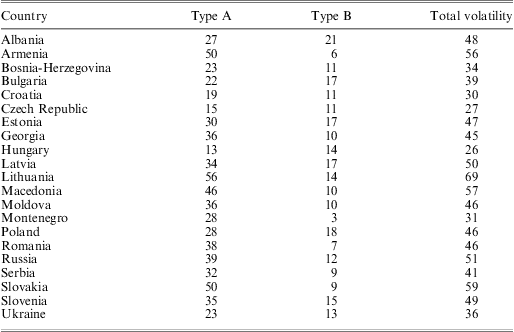
Across all the elections that met our criteria (that is, those displayed in Appendix Table A1), the mean level of Total Volatility is 45 per cent, Type A Volatility is just under 32 per cent and the mean level of Type B Volatility is just under 13 per cent. This finding illustrates that over 70 per cent of the Total Volatility in post-communist countries in this time period is Type A Volatility. The importance of this observation should not be understated. By contrast, in Western Europe during the same time period, almost two-thirds (60 per cent) of the Total Volatility comes from Type B Volatility. If this finding holds more broadly, and we can assume that the vast majority of electoral volatility in established democracies is of the Type B variety, this would mean that previous studies of electoral volatility in post-communist countries and established democracies were essentially analysing two different phenomena, despite the fact that they were employing the same measurement strategy (the Pedersen Index). Although for now we can only speculate about the nature of volatility across other regions of the world with newer competitive party systems, it seems quite legitimate to (at the very least) guess that there may be similar patterns at work there as well.

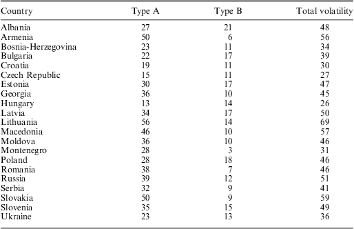
Table 1 (above) and Figure 1 (below) further disaggregate our data. Table 1 shows the mean volatility levels by country over time for the different types of volatility. For example in Slovakia, the mean level of Total Volatility (that is, what is calculated by the Pedersen Index) is 59 per cent. However, when broken into Type A Volatility and Type B Volatility, it becomes clear that almost all of Slovakia's volatility is due to Type A Volatility. We can also observe that the composition of Type A and Type B Volatility in Slovakia is quite different compared to that of Hungary, the only country with (barely) higher Type B Volatility than Type A Volatility.

Table 1

Mean Volatility by Country

Fig. 1

Deconstructed Type A and Type B volatility

Figure 1 illustrates the volatility scores by country for each election. (Each bar of the chart is a separate election; see Appendix Table A1 for election years). For a different way of visualizing these same data, see Appendix Figures A1, A2 and A3, which plot Type A Volatility, Type B Volatility and Total Volatility, respectively, over time.Footnote ²³

Taken together, we can make a number of interesting observations about patterns across the entire dataset, as well as within individual countries. Overall, we see that while both Type A Volatility and Total Volatility decrease over time, Type B Volatility is stable or increases slightly. These time trends suggest that these democracies may at some point start to resemble the more traditional volatility patterns of consolidated democracies as Type A Volatility fades and only Type B Volatility remains. Indeed, this is probably what we would expect to see as unstable new party systems gradually begin to solidify.

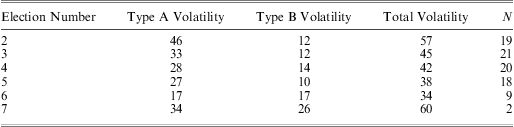
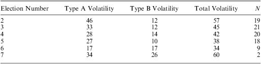
This time trend is also confirmed by looking at mean Type A, Type B and Total Volatility by time across countries. Specifically, Table 2 below shows mean volatility by election sequence and confirms the time trend shown in the figures. As countries have more elections, the level of Type A Volatility decreases, while the level of Type B Volatility slightly increases. (Note that the increase in Type A Volatility in the seventh election is based on only two cases). This pattern is consistent with a consolidating the party system, though the remaining levels of Type A Volatility suggest that there is still considerable progress yet to be made.

Table 2

Mean Volatility by Election Number

We can also use these data to examine volatility patterns within individual countries. For example, we can note that despite the overall trend, Type A Volatility is not declining in all countries. The clearest outlier to this general pattern is Lithuania, where the level of Type A Volatility increases quite substantially from 1996 to 2000, and even more so in 2004.Footnote ²⁴ We can also pick up patterns of countries in which Type A Volatility is itself volatile, such as Albania, which has very high levels of Type A Volatility in 1992 and 2005, but one of the lowest levels of Type A Volatility in 1996. Similar patterns can be found with Type B Volatility. Slovenia, for example, has high levels of Type B Volatility in 1996 and 2004, but a relatively low level in 2000. Alternatively, we can use the data to pick out elections that have particularly high levels of both Type A and Type B Volatility, such as Poland's transformational 2001 parliamentary elections.Footnote ²⁵ While a detailed explication of the reasons underlying changes in either Type A or Type B Volatility in any particular country is beyond the scope of this article, we hope these examples illustrate the kind of research questions that can be raised once we have quantitative measures of Type A and Type B Volatility by country and election year in hand.

Of course, we also now have the ability to examine whether traditional models of electoral volatility can explain variation in Type A and Type B volatility in post-communist countries, and it is to precisely this question that we turn in the following section.

Multivariate analyses of volatility

In this section, we use a standard volatility model to examine the effect of deconstructing Total Volatility into its Type A and Type B components in a multivariate framework. Our goal here is twofold. First, we want to see if we can recover a set of statistically significant predictors of electoral volatility when we rely only on the cases included in the Birch, Sikk and Tavits studies. Secondly, we want to examine whether these findings persist when we expand the size of the dataset, both by bringing it up to date and by fixing a firm rule for which countries to include in the analysis.Footnote ²⁶

As the Birch, Sikk and Tavits studies rely on different independent variables, we needed to arrive at a uniform set of regressors for our own analysis that contains variables that we would suspect could affect either Type A Volatility, Type B Volatility or both. As our primary goal in this article is not the development of new theoretical arguments, we do so by drawing on the framework presented in Mainwaring, Espana and Gervasoni, which essentially consists of three parts.Footnote ²⁷ The authors argue that volatility, and especially what they call ‘extra-system volatility’, ought to be more likely to emerge when (1) current government performance is poor, (2) the party system is more fragmented and (3) in the presence of formal institutional rules that make party entry easier. In addition, they suspect that extra-system volatility will decline over time.Footnote ²⁸

Our rationale behind including variables to tap into these three factors is as follows. First, poor government performance is expected to create an opportunity for new parties to capture the votes of former government supporters who may now be looking for a new champion. Poor government performance may also lead to more voters flowing away from the incumbent to established incumbent parties, and thus seems a good candidate for explaining both Type A and Type B volatility. Party system fragmentation – that is, the presence of more parties in the party system – ought to affect Type B volatility almost mechanically: the more parties there are, the more opportunities there are for party switching. Moreover, recent theoretical work has suggested that party systems with a higher number of political parties may make it easier for new party leaders to decide to introduce a new political party into the system without fear that there will be an adverse effect on policy outputs.Footnote ²⁹ Finally, if the decision underlying new party entry is guided by the non-policy costs of entry and conditioned on the likelihood of successfully winning votes in an election or seats in a parliament, then formal institutional barriers that either impose added costs on potential new parties or make success potentially less likely should have the effect of deterring potential new party entry, and thus should result in less Type A Volatility. These types of institutional barriers would not be expected, however, to affect Type B volatility.

Our statistical models therefore contain the following variables. To evaluate the question of government performance, we follow earlier studies in using macroeconomic conditions.Footnote ³⁰ Interestingly, most previous studies have only included short-term measures of macroeconomic performance, that is, changes in economic conditions since the previous election. However, in the post-communist context there is an obvious additional longer-term reference point against which people might compare the performance of the current government, which is how much better or worse the economy is performing now compared to under communism.Footnote ³¹ For this reason, our model includes change in GDP since the previous election as a measure of short-term economic performance, but also change in GDP since 1989, when communism collapsed in most of East-Central Europe, as a measure of government performance relative to the previous communist era.Footnote ³² Both measures are expected to tap into overall voter satisfaction with the performance of the current government.

To measure party system fractionalization, we take the standard tack of using the effective number of parties from the previous election.Footnote ³³ For formal institutions that have an effect on making entry easier or harder, we follow the standard pattern in the literature by including a measure of average district magnitude, which we log to account for the nature of countries with single national districts.Footnote ³⁴ The rational for doing so is explained in great detail in Cox, but the basic idea is that strategic voting leads to only M+1 candidate being viable in any given district, where M is the size of the district magnitude or the number of representatives per district. While there is no formal rule that prevents different parties from emerging to contest different districts, in most cases the same parties will do so in practice.Footnote ³⁵ Thus the larger the district magnitude, the more room there is in general for new party entry, and therefore the more ‘permissive’ the electoral system. According to Cox, whether a country also has an important elected president plays a role in determining whether the M + 1 rule results in the same M + 1 parties dominating throughout the country, so we also control for whether a country has a presidential, mixed or parliamentary system of government.Footnote ³⁶ Finally, it is widely agreed that proportional electoral rules make it easier for parties to achieve representation in parliament (Duverger's rule), so we also include whether or not a country employs proportional voting rules in its national legislative elections as a dummy variable in the model.Footnote ³⁷

In addition to the general categories suggested by the Mainwaring, Espana and Gervasoni framework,Footnote ³⁸ we also add two additional variables that have been shown to effect electoral volatility in previous studies of volatility in an effort to make sure that our models do not suffer from omitted variable bias. First, both Tavits and Sikk find an effect for time since democratization.Footnote ³⁹ In our models, we include both years since democratization and years since democratization squared (to allow time to have a non-linear effect on volatility). Secondly, ethnic fractionalization has been suggested to influence electoral volatility in studies outside of the post-communist region, although interestingly in some cases by dampening volatilityFootnote ⁴⁰ and in others by increasing volatility.Footnote ⁴¹

To test these hypotheses systematically on our different measures of volatility, we use a standard ordinary least square (OLS) regression model, but to take into account the fact that there may be unobserved heterogeneity in the standard errors within countries, we cluster our standard errors by country.Footnote ⁴² An alternative approach would have been to use a fixed-effects model rather than an OLS model. While this approach would have had the advantage of better addressing the panel nature of the data, it would have suffered from two additional problems. First, estimating additional parameters for the fixed-effects model would have further reduced our degrees of freedom and taxed our small number of cases substantially. Secondly, many of the most interesting theoretical explanations for variation in electoral volatility centre on variables that do not vary much within countries; a fixed-effects approach prevents us from studying them, or perhaps even worse, might identify effects based on a handful of cases that switch within a country.Footnote ⁴³ For a detailed description of these variables see Appendix Tables A2 and A3.

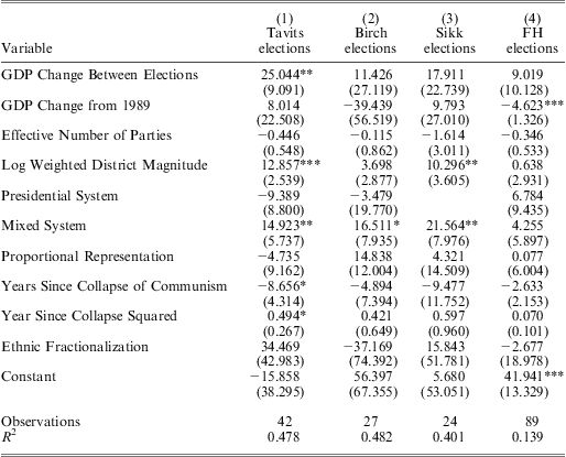
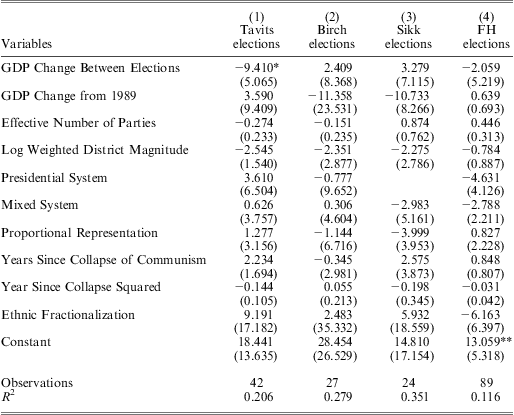
We begin with Type A (that is, party entry and exit) Volatility. Table 3 reports the results of our regression analysis of the covariates of Type A Volatility using the elections contained in the Tavits, Birch and Sikk studies, as well as the expanded dataset (FH elections) we have prepared. To reiterate, we are using the same data in all of the analyses; we vary only the elections included in each analysis to match the elections included in the earlier studies.

Table 3

Determinants of Type A Volatility by Case Selection

Note: standard errors clustered by country. Robust standard errors in brackets.

***p < 0.01, **p < 0.05, *p < 0.1.

When we restrict our analysis to the elections included in the Tavits study, we find a large number of statistically significant predictors of Type A Volatility, including GDP change between elections, the log weighted district magnitude, the governing system and (to a lesser extent) years since the collapse of communism. For the most part, the Birch and Sikk elections also reflect these findings, with (in most cases) coefficients of similar magnitude in similar directions, although we have a good deal less statistical confidence in these results (which is probably not surprising, given the smaller sample sizes); at the very least, though, they do not appear to be inconsistent with the Tavits findings.

In contrast, the FH Elections produce very different results. Of all the statistically significant variables in the Tavits analysis, not a single one survives when we increase our sample size to eighty-nine elections. Furthermore, a new variable emerges with strong explanatory power: GDP change since the collapse of communism. Thus we end up with a different explanation for Type A Volatility in post-communist countries. Far from being a response to barriers to entry, or short-term economic changes, variation in Type A Volatility in the first two decades of post-communist elections appears to be largely a function of the transition itself: Type A Volatility declines as the economy improves relative to where it was at the beginning of the transition. Thus something different is clearly going on in the expanded collection of elections as compared to the elections included in the Tavits study. A natural next question to ask, therefore, is whether this is a function of including more countries in the study, expanding the time frame of the study, or both.

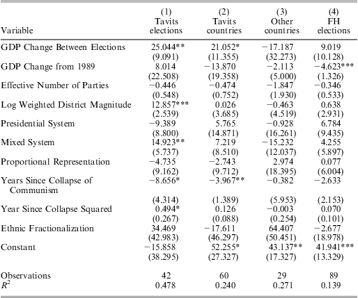
Table 4 demonstrates that the culprit appears to be expanding the scope of countries included in the study as opposed to the time frame of the analysis, although both are clearly having effects. The first and last columns of Table 4 are the same as in Table 3. The second column, however, replicates the analysis using all of the countries included in the Tavits analysis, but for all of the years in the FH Elections dataset, which increases the number of elections by roughly 50 per cent. The third column, in contrast, includes all of the elections from countries not included in the Tavits study. When we simply expand the time frame of the study in the original Tavits counties, we do find some similarities in the results (that is, between columns 1 and 2): GDP change between elections has roughly the same effect, and Type A Volatility still declines over time. In contrast, the size of the effect for both district size (Log Weighted District Magnitude) and having a mixed presidential/parliamentary system drops dramatically, and neither of these variables retains statistical significance at conventional levels. Turning to the twenty-nine elections from countries not included in the Tavits study, we find remarkably different patterns: none of the variables is statistically significant, and GDP change, district size and mixed governing systems all have coefficients in the opposite (albeit statistically insignificant) direction. So there is evidence that both expanding the time frame and expanding the number of countries in the analysis contribute to the new results, but the bottom line remains the same: determinants of Type A Volatility based on the analysis of elections included in the earlier studies are simply not robust to expanding the size of the dataset to those elections included in the FH Elections dataset.Footnote ⁴⁴

Table 4

Time or Countries? Type A Volatility

Note: standard errors clustered by country. Robust standard errors in brackets.

***p < 0.01, **p < 0.05, *p < 0.1.

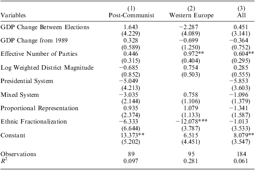
Turning to Type B Volatility, there is one overwhelming conclusion to be drawn from the results presented in Table 5: standard models of electoral volatility tell us little about what causes variation in electoral volatility between existing parties in post-communist countries. There is but a single statistically significant coefficient in the entire table, which with a significance level of 0.10 can of course be explained by chance alone. While it is possible that these findings are in some way a result of the particular choice of variables we used in our models, we have run many other specifications of these models and come to exactly the same conclusions.Footnote ⁴⁵ Moreover, in Table 3, we use the exact same variables – common in other analyses of electoral volatility – and find numerous statistically significant relationships, which suggests there is no underlying problem with the manner in which we code our independent variables.

Table 5

Determinants of Type B Volatility by Case Selection

Note: standard errors clustered by country. Robust standard errors in brackets.

***p < 0.01, **p < 0.05, *p < 0.1.

The one potential culprit we have not yet explored, however, is our coding of Type B Volatility. Although it seems unlikely, it remains possible that there is something about the way we coded this variable that is driving our null findings. Thus as a robustness test, we collected a parallel dataset in Western Europe from the same time period.

Table 6 presents the results of regressing Type B Volatility on a common set of variables in both Western Europe and the post-communist countries; note that we drop Time Since Communism from the analysis because this makes no sense in the West European context (which is why the results in Column 1 of Table 6 are not exactly the same as the results in Column 4 of Table 5). Here we do find two statistically significant predictors of Type B Volatility in Western Europe, suggesting that there is nothing inherent in the way we coded Type B volatility that precludes finding positive results. Interestingly, both of the variables that predict variation in Type B volatility in Western Europe – the effective number of parties and ethnic fractionalization – produce similar coefficients in the post-communist countries analysis, just of reduced size and with larger relative standard errors. This may suggest that there are common determinants of Type B volatility across old and new democracies, and that eventually once the amount of Type A Volatility begins to decline in the post-communist countries, we will be able to find similar explanations for overall levels of volatility across both regions.

Table 6

Determinants of Type B Volatility in Post-Communist Countries and Western Europe

Note: standard errors clustered by country. Robust standard errors in brackets.

***p < 0.01, **p < 0.05, *p < 0.1.

Taken together, it seems prudent to draw the following conclusions. To date, analyses of volatility in post-communist countries are essentially analyses of Type A Volatility; when we rerun our analyses in Tables 3 and 5 using Total Volatility (see Appendix Table A4), the results for Total Volatility closely resemble the results for Type A Volatility and look nothing like the results for Type B Volatility. Therefore any study that attempts to compare Total Volatility (that is, the Pedersen Index) in post-communist countries with Total Volatility in established democracies is essentially comparing two different political phenomenon; the former is dominated by variation in Type A Volatility and the latter is likely dominated by Type B Volatility. Thus unless one disaggregates electoral volatility into its Type A and Type B components, as we have done here, comparing Total Volatility in post-communist countries to Total Volatility in established democracies is essentially comparing apples to oranges.

Perhaps even more importantly, we suspect this is likely to be the case in new democracies the world over. At the very least, it ought to be incumbent upon scholars studying volatility in new democracies to identify what proportion of Total Volatility in those countries is due to Type A Volatility, and what proportion is due to Type B Volatility. This will at least allow us to understand how to interpret findings regarding Total Volatility (for example, in post-communist countries, Total Volatility is essentially Type A Volatility). A more noble longer-term goal would be to bring new theoretical insight to the topic by generating separate hypotheses for the analysis of Type A and Type B Volatility, a topic we return to in the following section.

Concluding thoughts: towards a new research agenda on electoral volatility

In this article, we have revisited the topic of electoral volatility in post-communist countries with a new and expanded dataset that includes all pairs of elections in post-communist countries from 1989–2009 that took place in countries rated at least ‘partially free’ by Freedom House. Building on observations from previous work, we develop an explicit framework for disaggregating the now well-known Pedersen Index into two separate components: volatility due to new party entry and exit (Type A Volatility) and volatility due to shifts in votes between existing parties (Type B Volatility). We also provide a set of detailed coding rules for measuring these two phenomena, as well as a broad overview of the prevalence of these two types of volatility during the first two decades of post-communist elections.

This exercise has allowed us to make four important conclusions concerning electoral volatility in post-communist countries. First, the story of electoral volatility in post-communist countries to date is largely one of Type A Volatility. This is the case whether we simply look at the amount of volatility caused by party entry/exit and compare it to volatility due to switching among existing parties, or if we conduct sophisticated multivariate analyses of determinants of volatility and observe similarities in the results across analyses of Type A and Total Volatility. Put simply, a study of Total Volatility in post-communist countries – at least to date – is primarily a study of Type A Volatility.

Second, while – in line with the findings of previous studies – we can indeed find statistically significant results when regressing Type A Volatility on a standard set of explanatory variables using a smaller number of elections included in earlier studies, these results almost entirely disappear in our expanded dataset. Patterns that were previously present seem no longer to be so.

With this general point in mind, our third conclusion is that, unlike previous studies of electoral volatility in post-communist countries, we find almost no support for the claim that structural factors such as district magnitude, electoral rules or ethnic heterogeneity affect levels of electoral volatility across elections, and only marginal evidence in support of the governing system. Nor does party system fractionalization seem to matter. Instead, we find just one statistically significant predictor of Type A Volatility over the first two decades of post-communist elections: the worse the economy is performing relative to where it was at the start of the transition, the more likely Type A volatility is to be high. Such a finding fits in very well with big-picture theoretical ideas about the extended role of the transition in structuring post-communist political behaviour:Footnote ⁴⁶ a country's long-term economic performance seems to create space for the creation of new political parties and incentives for failed ones to be abandoned.

It is, however, worth noting that in one of our robustness tests (Model 3 of Appendix Table A8), we found a strong positive effect for the number of years between elections on Type A volatility. Although not included in our original list of explanatory variables, there is a compelling logic at work here. The business of new party entry is time consuming, and in retrospect it does not necessarily seem surprising that the less time available to create a new party, the fewer successful new parties will emerge. It is a little more difficult to make a similar argument about party death, but if we think of loss of support as a somewhat linear cumulative process (as opposed, perhaps, to more of a tipping point model), then again we might suspect that in time, more dying parties might actually die. Either way, this strikes us as an interesting new theoretical direction for the study of Type A electoral volatility, and especially for new party entry.

Finally, we find that none of the extant theoretical explanations of electoral volatility give us any leverage into understanding variation in Type B electoral volatility in post-communist countries. We cannot really describe this as ‘contradicting’ previous studies, since, as noted above, previous studies that employed total volatility were really analysing Type A volatility. However it is very interesting to note that with a dataset that incorporates eighty-nine different pairs of elections from the collapse of communism to the present day, we really have no idea what explains the discrepancy in Type B volatility across different elections. Not only are none of these coefficients statistically significant, most are not even larger than their standard errors and many are in the wrong direction relative to expectations. Moreover, a wide range of tests of different specifications failed to budge us from this conclusion. To further test the credibility of these ‘negative’ findings, we collected a second dataset containing all elections in Western Europe during the same time period. Here we were able to find statistically significant results, thus decreasing our concern that there might be something inherently problematic with our measurement strategy.

One feature of our analysis is that we applied the same model to analyse Type A and Type B Volatility. We have good reasons for doing so in the context of this article – we were explicitly comparing results from similar models using different numbers of elections – but one exciting prospect for further study of electoral volatility, especially outside the confines of established democracies, would be to begin to think theoretically about the factors that ought to effect Type A Volatility but not Type B Volatility, those that ought to effect Type B Volatility but not Type A Volatility, and those that might effect both.

Consider as one example the state of the economy, which has often been present on the right-hand side of analyses of electoral volatility. Theories of economic voting suggest that we might see an excessive movement of voters away from the incumbent party if the economy performs particularly poorly, but also that we might see large numbers of voters switching their vote to the incumbent party if the economy performs particularly well. In both cases, therefore, we might expect higher Type B Volatility than if the economy performs about average. So a theoretically appropriate economic variable for explaining Type B Volatility might be ‘deviation in economic experience’, or some sort of measure of how the economy is performing this year relative to its average performance, be it exceptionally good or bad. In contrast, however, we would hardly expect elites to expend effort forming a new party if they believe the incumbent party will cruise to victory because of an exceptionally strong economy. We might, however, expect elites to form new parties if the economy was performing particularly poorly, with the expectation that dissatisfied supporters of that party could be looking for a new home in the upcoming election. Thus a theoretically appropriate economic variable to study Type A Volatility might be one that captures only the worst-performing economies.

We can also apply similar thinking to institutional variables. For example, a higher minimum necessary vote threshold for receiving seats in proportional representation voting systems ought to have a strong effect on dissuading new party entry, but ought not to make much of a difference in how much voters are likely to shift between three dominant parties in a three-party system. Thus it might be theoretically appropriate to include a measure of the electoral threshold in a study of Type A Volatility, but we might not have any reason to want to include a similar variable in a study of Type B Volatility.

We might also be able to think creatively about the way that past experiences could affect the different types of electoral volatility. For example, elites might be more likely to think a new party would enjoy electoral success the less attached they thought voters were to the parties they had voted for in the previous election. Thus an election which featured high Type B Volatility might have the effect of convincing elites that voter loyalties to their current parties are weak, and therefore that the ensuing election might be a good time to start a new party. With this in mind, we might want to include lagged Type B Volatility in a model predicting Type A Volatility.Footnote ⁴⁷

Once we have these theoretically appropriate models for Type A and Type B Volatility in hand, we can also begin to think about interesting cross-regional applications. Simple descriptive statistics would certainly be an interesting place to start. Based on our own preliminary research we know that there are much, much higher levels of Type A Volatility in Eastern Europe than in Western Europe over the same time period, but how might Africa and Latin America compare? Indeed, it may turn out that Type A Volatility is more important than Type B Volatility for determining party system stability in most parts of the world, although this could also end up having a threshold effect: perhaps once Type A Volatility falls below a certain level, Type B Volatility becomes more important. It would also be interesting to learn whether the same factors that explain Type B Volatility in established democracies also do so in newer democracies. Perhaps we'll even end up needing models tailored to different factors in new democracies (based on low information about parties) vs. established democracies (based on high information about parties) for Type B Volatility, but not for Type A Volatility (since in both cases little will be known about these new parties). From an empirical standpoint, it would be interesting to know whether different factors affect Type A Volatility in different political contexts. Perhaps the factors that guide successful new party entry and exit will turn out to be different in post-communist societies with strong communist successor parties than in African countries where there are strong ties between ethnic groups and political parties.

All of these questions – and many others not considered here – strike us as both empirically interesting and fertile ground for theory building. What they have in common, though, is that they all build on the fact that the current measure of electoral volatility in the discipline, the Pedersen Index, conflates two essentially different forms of volatility. By highlighting a simple new conceptual tool – the idea of Type A and Type B electoral volatility – we hope to suggest a solution to this problem and an important step forward in research on electoral volatility.