1 Introduction
In aerodynamic applications, flow separation can cause detrimental effects such as stall. Flow separation can also intensify the pressure fluctuation and cause structural fatigue. For these reasons, suppression of flow separation over aerodynamic bodies has been an area of focus for the flow control community (Joslin & Miller Reference Joslin and Miller2009). Active flow control, which requires steady or unsteady input of external energy, is capable of adapting to a wide range of operating conditions. It has the advantage over passive control strategies whose performance can degrade in off-design conditions. For separation control, in particular, unsteady forcing has demonstrated its enhanced capability of reattaching the flow and improving aerodynamic performances (Zaman, McKinzie & Rumsey Reference Zaman, McKinzie and Rumsey1989; Wu et al. Reference Wu, Lu, Denny, Fan and Wu1998). Consequently, attempts have been made to investigate the effect of different unsteady forcing frequencies on control (Seifert & Pack Reference Seifert and Pack1999; Glezer, Amitay & Honohan Reference Glezer, Amitay and Honohan2005). A range of flow responses to forcing frequency were examined by conducting parametric studies of separation control (Amitay & Glezer Reference Amitay and Glezer2002). However, the characterization of global frequency response of the separated flow lacks quantitative support from theoretical analyses. Moreover, detailed knowledge of effective frequency range for unsteady separation control remains limited.
Greenblatt & Wygnanski (Reference Greenblatt and Wygnanski2000) provided an overview on the use of periodic excitation for separation control. They suggested that the fundamental mechanism for suppression of separation lies in the excitation of the Kelvin–Helmholtz instabilities in the shear layer forming from the separation point. The seminal work of Brown & Roshko (Reference Brown and Roshko1974) pointed out that the formation of spanwise coherent structures due to these instabilities is the main driving force for the momentum mixing and entrainment. Leveraging the shear-layer instabilities has been an important strategy to suppress flow separation (Joslin & Miller Reference Joslin and Miller2009). As such, knowledge on the instability and receptivity of the separated flow is crucial to guide the design of active separation control.
For the study of hydrodynamic instability, a variety of approaches have been summarized by Schmid & Henningson (Reference Schmid and Henningson2001) and Theofilis (Reference Theofilis2011). One traditional approach for analysing instability seeks a modal representation for infinitesimal perturbations about an equilibrium base state, i.e. a solution to the Navier–Stokes equations. Such an approach forms an eigenvalue problem for the global instability modes and emphasizes the spectrum of the linearized Navier–Stokes operator (Barkley & Henderson Reference Barkley and Henderson1996; Sipp & Lebedev Reference Sipp and Lebedev2007; Liu, Gómez & Theofilis Reference Liu, Gómez and Theofilis2016; Sun et al. Reference Sun, Taira, Cattafesta and Ukeiley2017; Taira et al. Reference Taira, Brunton, Dawson, Rowley, Colonius, McKeon, Schmidt, Gordeyev, Theofilis and Ukeiley2017). Inherently, it characterizes the asymptotic long-time behaviour of the perturbations about the base flow. Complementing this traditional approach, the non-modal approach addresses flow instability by seeking an energy measure for the time-evolving response of the flow (Schmid Reference Schmid2007). The non-modal approach either forms an initial-value problem that examines the transient energy growth over a finite-time window (Schmid & Rossi Reference Schmid and Rossi2004), or investigates the energy amplification from a harmonic forcing input to the harmonic response (Farrell & Ioannou Reference Farrell and Ioannou1993; Trefethen et al. Reference Trefethen, Trefethen, Reddy and Driscoll1993; Jovanović & Bamieh Reference Jovanović and Bamieh2005). The latter path is closely related to receptivity analysis (Goldstein & Hultgren Reference Goldstein and Hultgren1989; Choudhari Reference Choudhari1993), and has built the foundation for the resolvent analysis extended for turbulent flows.
With recent developments, resolvent analysis has become a valuable approach for investigating the frequency response of a fluid-flow system. Resolvent analysis is concerned with the pseudospectrum of a linear operator (Trefethen & Embree Reference Trefethen and Embree2005). It provides particularly valuable insights when the linear operator is non-normal, which is encountered in shear-dominated flows (Schmid & Henningson Reference Schmid and Henningson2001). Trefethen et al. (Reference Trefethen, Trefethen, Reddy and Driscoll1993) conducted such an analysis on laminar Poiseuille flows. They showed that the perturbation energy can exhibit significant transient growth due to the non-normality of the operator. This growth can depart from the linear regime and cause subcritical laminar–turbulent transition. For a non-normal operator, a linear mechanism of pseudoresonance can also result in a large resonant behaviour to forcing even when the forcing frequency is far from the spectrum (eigenvalues) of the operator. McKeon & Sharma (Reference McKeon and Sharma2010) extended the resolvent analysis for turbulent flows. The challenge in formulating the analysis for turbulent mean flow stems from the nonlinear terms of finite-amplitude perturbations. In their framework, these nonlinear terms are treated as internal forcing, yielding a linear relationship between the nonlinearity and the harmonic flow response. The linear relationship describes an input–output process that takes place through the resolvent operator constructed about the statistically stationery turbulent mean flow. By examining the characteristics of the resolvent operator, they captured the coherent structures in wall-bounded turbulence, revealing scalings for length and velocity that are in agreement with experimental measurements. Following this resolvent formulation, similar approaches have been undertaken in numerous studies (Moarref et al. Reference Moarref, Sharma, Tropp and McKeon2013; Beneddine et al. Reference Beneddine, Sipp, Arnault, Dandois and Lesshafft2016; Gómez et al. Reference Gómez, Blackburn, Rudman, Sharma and McKeon2016).
Resolvent analysis, as an input–output analysis, gives knowledge of energy amplification as well as the associated structural response to the perturbation over a range of frequencies. Such knowledge is crucial in designing active flow control techniques, because both amplification and response structure provide insights into identifying the effective unsteady forcing that takes minimal energy to change the mean flow. Applying this analysis to turbulent flows, our study aims to provide theoretical support to examine the flow response under unsteady forcing and to develop a predictive tool for identifying the range of effective actuation frequencies. In this study, we conduct an active flow control effort combining large-eddy simulations (LES) and resolvent analysis of the mean baseline flows over a canonical airfoil. Over the airfoil, the control input is introduced in the form of local periodic heat injection near the leading edge. We parameterize the actuation frequency and spanwise wavenumber in this numerical effort. Our choice of thermal actuator is motivated by the energy-based actuators that have become widespread in active flow control, such as nanosecond pulse-driven dielectric barrier discharge plasma actuators (Little et al. Reference Little, Takashima, Nishihara, Adamovich and Samimy2012) and thermoacoustic actuators (Yeh et al. Reference Yeh, Munday, Taira and Munson2015). These energy-based actuators have a sheet-like arrangement with no moving parts, which allows for a surface-compliant installation without occupying any internal space or adding significant weight. The thermal actuator set-up used in the present study models the thermoacoustic and plasma-based actuators at a fundamental level (Bin, Oates & Taira Reference Bin, Oates and Taira2015; Chae et al. Reference Chae, Ahn, Kim and Kim2017).
Resolvent analysis has been conducted on flows over a NACA 0012 airfoil in a similar effort by Thomareis & Papadakis (Reference Thomareis and Papadakis2018). They selected turbulent mean flow over the airfoil at
 $5^{\circ }$
angle of attack and at a chord-based Reynolds number of
 $50\,000$
as the base state for their analysis, and considered resolvent analysis to capture the frequency spectra of probe measurements. According to the forcing mode structures, they also showed that the flow exhibits high receptivity near the leading edge. With their base flow likely being unstable, one should infer the physical implications of resolvent analysis with great care. For unstable base flows, the significance of input–output amplification would be shadowed by the unbounded perturbation growth in the linearized formulation. For this reason, the present effort carefully considers the stability of the base flow and raises the need for an appropriate time window for the resolvent analysis. The stability characteristics of the chosen base flow are examined prior to the performance of resolvent analysis and provide an upper bound on the time window. In particular, we discuss the use of a temporal filter in the form of an exponential discount (Jovanović Reference Jovanović2004).
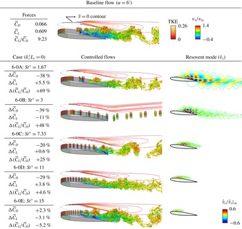
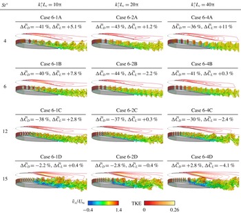
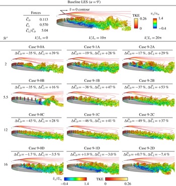
A roadmap of this study is outlined in figure 1. Starting in § 2, we perform the baseline flow simulations at two post-stall angles of attack. The baseline flows are validated and characterized. With the turbulent mean flow obtained from the baseline LES, the global resolvent operator is constructed about the time- and spanwise-averaged mean flow at a specified wavenumber–frequency combination in § 3. Resolvent analysis performs a singular value decomposition (SVD) of the discrete resolvent operator to determine the forcing modes, response modes and the associated amplification (gain). The amplification as well as the modal structures are characterized over the Fourier space, so as to obtain physical insights into the candidate range of actuation frequencies and wavenumbers for active flow control to suppress flow separation. In § 4, we present the LES results of over 250 controlled cases using open-loop actuation with different actuation frequencies and wavenumbers. The control effects are quantified and compared to the prediction of resolvent analysis on the mean baseline flows. We comment on the agreements and limitations of the usage of resolvent analysis for design of active flow control in § 5.
Roadmap of the present study.

2 Problem set-up
2.1 Problem description
We consider separated flows over a NACA 0012 airfoil at two angles of attack of
 $\unicode[STIX]{x1D6FC}=6^{\circ }$
and
 $9^{\circ }$
for a moderate chord-based Reynolds number
 $Re_{L_{c}}\equiv v_{\infty }L_{c}/\unicode[STIX]{x1D708}_{\infty }=23\,000$
and a free-stream Mach number
 $M_{\infty }\equiv v_{\infty }/a_{\infty }=0.3$
, as shown in figure 2. Here,
 $v_{\infty }$
is the free-stream velocity,
 $L_{c}$
is the chord length,
 $a_{\infty }$
is the free-stream sonic speed and
 $\unicode[STIX]{x1D708}_{\infty }$
is the kinematic viscosity. To perform active flow control, a thermal actuator is placed across the span near the leading edge. This actuator introduces oscillatory heat flux at a prescribed frequency and spanwise profile as an open-loop actuation input. The details of this thermal actuator will be discussed in § 2.3.
2.2 Simulation set-up
The problem description. Separated flow over a NACA 0012 airfoil (shown for
 $\unicode[STIX]{x1D6FC}=6^{\circ }$
) at free-stream Mach number
 $M_{\infty }=0.3$
and chord-based Reynolds number
 $Re_{L_{c}}=23\,000$
.

We perform LES to simulate spanwise-periodic flows over the airfoil using the finite-volume compressible flow solver CharLES (Khalighi et al.
Reference Khalighi, Nichols, Ham, Lele and Moin2011; Brès et al.
Reference Brès, Ham, Nichols and Lele2017), which is second-order accurate in space and third-order accurate in time. Vremen’s subgrid-scale model (Vreman Reference Vreman2004) is utilized in the LES. We utilize a C-shaped computational mesh, with the airfoil positioned with its leading edge at
 $x/L_{c}=y/L_{c}=0$
, as shown in figure 3. The extent of the computational domain is
 $x/L_{c}\in [-19,26]$
,
 $y/L_{c}\in [-20,20]$
and
 $z/L_{c}\in [-0.1,0.1]$
in the streamwise, transverse and spanwise directions, respectively. This domain is discretized with approximately 35 million grid cells. We have examined the grid convergence by comparing the flow field and aerodynamics forces from this mesh to two other meshes that are further refined in the near field with a total of 63 and 82 million grid cells. From each mesh, the force data are collected for the developed flow over 80 convective time units. The time-averaged wall-normal velocity profiles were converged within
 $1.5\,\%$
and aerodynamic forces were also observed to be insensitive to the grid resolution of the three meshes.
For the fluid properties, we use the specific heat ratio
 $\unicode[STIX]{x1D6FE}=1.4$
and the Prandtl number
 $Pr=0.7$
, which are representative for standard air. The temperature-varying dynamic viscosity,
 $\unicode[STIX]{x1D707}(T)$
, is evaluated with a power law as
 $\unicode[STIX]{x1D707}=\unicode[STIX]{x1D707}_{\infty }(T/T_{\infty })^{0.76}$
, where
 $\unicode[STIX]{x1D707}_{\infty }$
and
 $T_{\infty }$
are the free-stream dynamic viscosity and temperature, respectively (Garnier, Adams & Sagaut Reference Garnier, Adams and Sagaut2009). The power law models the dynamic viscosity variation for standard air in the range
 $T/T_{\infty }\in [0.5,1.7]$
. This range is suitable for the current study with local thermal inputs, where we observe that the maximum temperature fluctuation is within
 $42\,\%$
of
 $T_{\infty }$
for all controlled flows.
The computational domains (
 $x$
–
 $y$
plane, shown for
 $\unicode[STIX]{x1D6FC}=6^{\circ }$
) for LES and resolvent analysis. The near-field mesh (right) is shown along with instantaneous spanwise vorticity from LES and streamwise velocity mode from resolvent analysis. For both meshes, uniform
 $\unicode[STIX]{x0394}x$
is adopted in
 $x/L_{c}\in [1.5,6]$
to resolve the wake structures.

The simulations are performed with the Dirichlet boundary condition specified at the far-field boundary as
 $[\unicode[STIX]{x1D70C},v_{x},v_{y},v_{z},T]=[\unicode[STIX]{x1D70C}_{\infty },v_{\infty },0,0,T_{\infty }]$
, where
 $\unicode[STIX]{x1D70C}$
is the density,
 $v_{x}$
,
 $v_{y}$
and
 $v_{z}$
are respectively the streamwise, transverse and spanwise velocities and
 $T$
is the temperature. Over the airfoil, the no-slip adiabatic boundary condition is prescribed, except for where the actuator is placed for controlled cases. Along the outlet boundary, a sponge layer (Freund Reference Freund1997) is applied over
 $x/L_{c}\in [15,25]$
with the target state set to the running-averaged flow over 10 acoustic time units. Time integration is performed at a constant time step of
 $\unicode[STIX]{x0394}tv_{\infty }/L_{c}=4.14\times 10^{-5}$
, corresponding to a maximum Courant–Friedrichs–Lewy number of
 $0.84$
. Further details regarding the meshing strategy and computational set-up are reported in Yeh, Munday & Taira (Reference Yeh, Munday and Taira2017a
).
2.3 Actuator model
The thermal actuator is implemented as an oscillatory energy-flux boundary condition to model the fundamental effects of thermoacoustic and plasma-based actuators in the LES. It is prescribed in the energy equation as an unsteady Neumann boundary condition, along with no-slip boundary condition for the momentum equation in the compressible Navier–Stokes equations. The actuator model is expressed as
 $$\begin{eqnarray}\displaystyle \unicode[STIX]{x1D719}^{+}(\unicode[STIX]{x1D714}^{+},k_{z}^{+})=\frac{1}{4}\hat{\unicode[STIX]{x1D719}}\sin (\unicode[STIX]{x1D714}^{+}t)[1+\cos (k_{z}^{+}z)]\left\{1+\cos \left[\frac{2\unicode[STIX]{x03C0}}{\unicode[STIX]{x1D70E}_{a}}(x-x_{a})\right]\right\}, & & \displaystyle\end{eqnarray}$$
where
 $(x-x_{a})/\unicode[STIX]{x1D70E}_{a}\in [-0.5,0.5]$
. This expression provides the boundary heat flux input with a compact spatial support in the form of a Hanning window centred at
 $x_{a}/L_{c}=0.03$
on the suction surface with width of
 $\unicode[STIX]{x1D70E}_{a}/L_{c}=0.04$
, as illustrated in figure 2. The actuator introduces the open-loop control input at the prescribed actuation frequency,
 $\unicode[STIX]{x1D714}^{+}$
, and spanwise wavenumber,
 $k_{z}^{+}$
. They are parameterized in the LES of controlled cases and reported in terms of the actuation Strouhal number
 $St^{+}=\unicode[STIX]{x1D714}^{+}L_{c}/(2\unicode[STIX]{x03C0}v_{\infty })$
and the normalized wavenumber
 $k_{z}^{+}L_{c}$
throughout this paper. Due to the choice of the spanwise extent for the computational domain (
 $z/L_{c}\in [-0.1,0.1]$
), the actuation wavenumbers
 $k_{z}^{+}L_{c}$
are restricted to integer multiples of
 $10\unicode[STIX]{x03C0}$
. Hence, we only consider the use of
 $k_{z}^{+}L_{c}=0$
,
 $10\unicode[STIX]{x03C0}$
,
 $20\unicode[STIX]{x03C0}$
and
 $40\unicode[STIX]{x03C0}$
in the LES of controlled flows. In the actuator model (2.1), the actuation amplitude
 $\hat{\unicode[STIX]{x1D719}}$
is selected such that the normalized total actuation power
 $$\begin{eqnarray}\displaystyle E^{+}=\frac{\frac{1}{4}\hat{\unicode[STIX]{x1D719}}\unicode[STIX]{x1D70E}_{a}}{\frac{1}{2}\unicode[STIX]{x1D70C}_{\infty }v_{\infty }^{3}(L_{c}\sin \unicode[STIX]{x1D6FC})}=0.0902 & & \displaystyle\end{eqnarray}$$
for all controlled cases throughout this work. This magnitude is representative of those used in thermally actuated flow control studies (Corke, Enloe & Wilkinson Reference Corke, Enloe and Wilkinson2010; Sinha et al. Reference Sinha, Alkandry, Kearney-Fischer, Samimy and Colonius2012; Akins, Singh & Little Reference Akins, Singh and Little2015; Yeh et al. Reference Yeh, Munday, Taira and Munson2015). For this thermal actuator, Yeh, Munday & Taira (Reference Yeh, Munday and Taira2017b ) have investigated its control mechanism and flow control capability in free shear layers. The thermal input from the actuator translates to vortical perturbations in the forms of oscillatory surface vorticity flux and baroclinic torque. The thermal actuation is capable of exciting fundamental and subharmonic instabilities, which is suitable for modifying the shear-layer dynamics herein.
2.4 Baseline simulations
We validate the baseline simulations at angles of attack of
 $\unicode[STIX]{x1D6FC}=6^{\circ }$
and
 $9^{\circ }$
by comparing the surface pressure distribution and the aerodynamic forces to those reported in the literature for
 $Re_{L_{c}}=23\,000$
. Throughout this study, the pressure coefficient
 $C_{p}$
, lift coefficient
 $C_{L}$
and drag coefficients
 $C_{D}$
are defined as
 $$\begin{eqnarray}\displaystyle C_{p}=\frac{p-p_{\infty }}{\frac{1}{2}\unicode[STIX]{x1D70C}_{\infty }v_{\infty }^{2}},\quad C_{L}=\frac{F_{L}}{\frac{1}{2}\unicode[STIX]{x1D70C}_{\infty }v_{\infty }^{2}A},\quad C_{D}=\frac{F_{D}}{\frac{1}{2}\unicode[STIX]{x1D70C}_{\infty }v_{\infty }^{2}A}, & & \displaystyle\end{eqnarray}$$
where
 $F_{L}$
and
 $F_{D}$
are the total lift and drag forces on the airfoil, respectively, and
 $A$
is the planform area of the airfoil. The time-averaged aerodynamic forces and surface pressure profile are respectively presented in table 1 and figure 4. We found reasonable agreements with those reported by Kim et al. (Reference Kim, Yang, Chang and Chung2009), Kojima et al. (Reference Kojima, Nonomura, Oyama and Fujii2013) and Munday & Taira (Reference Munday and Taira2018). We note that the numerical study of Kojima et al. (Reference Kojima, Nonomura, Oyama and Fujii2013) was conducted using implicit LES and Munday & Taira (Reference Munday and Taira2018) reported the results from incompressible LES. The discrepancy in the surface pressure with the experimental measurement by Kim et al. (Reference Kim, Yang, Chang and Chung2009) can be attributed to the different transverse blockage ratios (
 $0.26\,\%$
for the present study).
The time-averaged drag and lift coefficients on a NACA 0012 airfoil at
 $\unicode[STIX]{x1D6FC}=6^{\circ }$
and
 $9^{\circ }$
at
 $Re_{L_{c}}=23\,000$
. The present study performs compressible LES at a free-stream Mach number
 $M_{\infty }=0.3$
, in comparison with the results from incompressible LES by Munday & Taira (Reference Munday and Taira2018) and implicit LES by Kojima et al. (Reference Kojima, Nonomura, Oyama and Fujii2013) at
 $M_{\infty }=0.2$
.

Surface pressure profiles for (a)
 $\unicode[STIX]{x1D6FC}=6^{\circ }$
and (b)
 $\unicode[STIX]{x1D6FC}=9^{\circ }$
over the chord-wise coordinate
 $x_{c}/L_{c}=(x\cos \unicode[STIX]{x1D6FC}+y\sin \unicode[STIX]{x1D6FC})/L_{c}$
, in comparison with those reported by Kim et al. (Reference Kim, Yang, Chang and Chung2009), Kojima et al. (Reference Kojima, Nonomura, Oyama and Fujii2013) and Munday & Taira (Reference Munday and Taira2018).

(a,b) Baseline flow visualization using
 $Q$
-criterion (iso-surface of
 $QL_{c}^{2}/v_{\infty }^{2}=50$
coloured by streamwise velocity) and spanwise-average
 $\text{TKE}=\overline{(v_{x}^{\prime 2}+v_{y}^{\prime 2}+v_{z}^{\prime 2})}/v_{\infty }^{2}$
in the background. (c,d) The time-averaged streamlines. The contour line for
 $\bar{v}_{x}=0$
is shown and will be used for characterizing the extent of the separation region throughout this study.

The instantaneous flow fields and time-average streamlines for the baseline flows at
 $\unicode[STIX]{x1D6FC}=6^{\circ }$
and
 $9^{\circ }$
are shown in figure 5. The iso-surface of
 $Q$
-criterion (Hunt, Wray & Moin Reference Hunt, Wray and Moin1988) is used to visualize the vortical structures. The contour line of time- and spanwise-averaged streamwise velocity
 $\bar{v}_{x}=0$
is also shown to identify the flow separation and reattachment. This contour line is also shown on top of the time-average streamlines, where we see the contour line extends through the separation bubble for each case. For both angles of attack, laminar separation is observed near the leading edge and forms a shear layer. The shear layer rolls up over the suction surface and evolves into spanwise vortices. This roll-up process leads to increasing turbulent kinetic energy (TKE) within the shear layer. Farther downstream, these spanwise vortices break up and lose their spanwise coherence, resulting in the laminar–turbulent transition. Within this roll-up and transition process, one common feature in the pressure profiles in figure 4 is the ‘plateau’ observed for both angles of attack. Such a plateau in the pressure profile is also observed by Marxen, Lang & Rist (Reference Marxen, Lang and Rist2013) and Benton & Visbal (Reference Benton and Visbal2018) in the transition process that takes place over a laminar separation bubble. The transition process is accompanied by the maximum TKE over the airfoil at
 $x/L_{c}\approx 0.6$
for
 $\unicode[STIX]{x1D6FC}=6^{\circ }$
and
 $x/L_{c}\approx 0.5$
for
 $\unicode[STIX]{x1D6FC}=9^{\circ }$
. The roll-up and break-up processes both result in momentum mixing and entraining of the free stream, leading to flow reattachment for
 $\unicode[STIX]{x1D6FC}=6^{\circ }$
at
 $x/L_{c}\approx 0.85$
. Over the airfoil at
 $\unicode[STIX]{x1D6FC}=9^{\circ }$
, the flow is in full stall. To quantitatively characterize the stall condition, we calculate the potential-flow lift
 $C_{L,0}$
using the panel method (Hess Reference Hess1990) to mark a theoretical upper bound of the lift for both angles of attack. The flow over the airfoil at
 $\unicode[STIX]{x1D6FC}=6^{\circ }$
reattaches and achieves
 $84\,\%$
of
 $C_{L,0}$
. Whereas for the
 $\unicode[STIX]{x1D6FC}=9^{\circ }$
airfoil, while experiencing deep stall, provides only
 $52\,\%$
of the potential flow lift. This difference in the stall condition will be reflected in the control effectiveness to be discussed in § 4.
The excitation of shear-layer instabilities serves as the key to separation control (Greenblatt & Wygnanski Reference Greenblatt and Wygnanski2000). For the laminar separation bubble that is observed in both baseline flows, Häggmark, Bakchinov & Alfredsson (Reference Häggmark, Bakchinov and Alfredsson2000) have experimentally shown that the Kelvin–Helmholtz instability dominates the laminar–turbulent transition. In order to leverage the Kelvin–Helmholtz instability for flow control, we place the thermal actuator slightly upstream of the separation point such that the perturbations can be introduced at the onset of the shear layer.
3 Resolvent analysis of mean baseline flows
Following the baseline LES, we perform resolvent analysis of the mean turbulent flows at
 $\unicode[STIX]{x1D6FC}=6^{\circ }$
and
 $9^{\circ }$
to provide physical insights into the design of active separation control.
3.1 Formulation
Let us consider the compressible Navier–Stokes equations expressed as
 $$\begin{eqnarray}\displaystyle \frac{\unicode[STIX]{x2202}\boldsymbol{q}}{\unicode[STIX]{x2202}t}={\mathcal{N}}(\boldsymbol{q})+\boldsymbol{f}^{+}, & & \displaystyle\end{eqnarray}$$
where
 ${\mathcal{N}}$
is the nonlinear Navier–Stokes operator that acts on the flow state variable
 $\boldsymbol{q}=[\unicode[STIX]{x1D70C},v_{x},v_{y},v_{z},T]^{\text{T}}$
and
 $\boldsymbol{f}^{+}$
represents the external actuation input from active flow control. Note that in general the external forcing
 $\boldsymbol{f}^{+}$
can be absent. We perform the Reynolds decomposition of
 $\boldsymbol{q}=\bar{\boldsymbol{q}}+\check{\boldsymbol{q}}$
so that the flow state variable
 $\boldsymbol{q}$
is decomposed into a statistically stationary long-time mean component
 $\bar{\boldsymbol{q}}$
and a fluctuating component
 $\check{\boldsymbol{q}}$
. Substituting
 $\boldsymbol{q}$
with its Reynolds decomposition into the Navier–Stokes equations (3.1) yields
 $$\begin{eqnarray}\displaystyle \frac{\unicode[STIX]{x2202}\bar{\boldsymbol{q}}}{\unicode[STIX]{x2202}t}+\frac{\unicode[STIX]{x2202}\check{\boldsymbol{q}}}{\unicode[STIX]{x2202}t}=\underbrace{{\mathcal{L}}(\check{\boldsymbol{q}},\bar{\boldsymbol{q}}\unicode[STIX]{x1D735}\check{\boldsymbol{q}},\check{\boldsymbol{q}}\unicode[STIX]{x1D735}\bar{\boldsymbol{q}},\unicode[STIX]{x1D6FB}^{2}\check{\boldsymbol{q}},\cdots \,)}_{{\mathcal{L}}_{\bar{\boldsymbol{ q}}}(\check{\boldsymbol{q}})}+\underbrace{{\mathcal{N}}(\bar{\boldsymbol{q}})+\bar{f}(\check{\boldsymbol{q}}^{n})+\boldsymbol{f}^{+}}_{\check{\boldsymbol{u}}}. & & \displaystyle\end{eqnarray}$$
With the Reynolds decomposition, the linear operations for
 $\check{\boldsymbol{q}}$
are extracted from the operation of
 ${\mathcal{N}}(\bar{\boldsymbol{q}}+\check{\boldsymbol{q}})$
. We collect these terms that are linear with respect to
 $\check{\boldsymbol{q}}$
and denote them as
 ${\mathcal{L}}_{\bar{\boldsymbol{q}}}(\check{\boldsymbol{q}})$
. The term
 ${\mathcal{N}}(\bar{\boldsymbol{q}})$
accounts for the Navier–Stokes operation taking place only on
 $\bar{\boldsymbol{q}}$
, and
 $\bar{f}(\check{\boldsymbol{q}}^{n})$
collects the nonlinear higher-order terms for
 $\check{\boldsymbol{q}}$
in
 $O(\boldsymbol{q}^{n})$
, where
 $n>1$
. In particular, we note that
 ${\mathcal{N}}(\bar{\boldsymbol{q}})+\bar{f}(\check{\boldsymbol{q}}^{n})$
can be interpreted as the internal forcing in the turbulent flow due to the nonlinear interaction (Farrell & Ioannou Reference Farrell and Ioannou1994; McKeon & Sharma Reference McKeon and Sharma2010). This internal forcing together with the external forcing
 $\boldsymbol{f}^{+}$
is further denoted as
 $\check{\boldsymbol{u}}$
. Observing that the base flow is taken to be time-invariant, i.e.
 $\unicode[STIX]{x2202}_{t}\bar{\boldsymbol{q}}=0$
, equation (3.2) can be simplified as
 $$\begin{eqnarray}\displaystyle \frac{\unicode[STIX]{x2202}\check{\boldsymbol{q}}}{\unicode[STIX]{x2202}t}={\mathcal{L}}_{\bar{\boldsymbol{q}}}(\check{\boldsymbol{q}})+\check{\boldsymbol{u}}. & & \displaystyle\end{eqnarray}$$
We note that, for a statistically stationary turbulent flow where
 $\bar{\boldsymbol{q}}$
is known a priori and is not affected by the sustained forcing input
 $\check{\boldsymbol{u}}$
, the linear operator
 ${\mathcal{L}}_{\bar{\boldsymbol{q}}}$
is also time-invariant and can be explicitly constructed with the knowledge of
 $\bar{\boldsymbol{q}}$
. Therefore, equation (3.3) can be viewed as a linear system for
 $\check{\boldsymbol{q}}$
. The nonlinear interaction in
 $\check{\boldsymbol{u}}$
supports the base flow
 $\bar{\boldsymbol{q}}$
via its mean component and forces
 $\check{\boldsymbol{q}}$
with its fluctuating component (McKeon & Sharma Reference McKeon and Sharma2010). Thus far, no assumptions have been made in the formulation except for the statistical stationarity of the turbulent flow about which the Navier–Stokes equations are rewritten in the above form.
Now, we cast equation (3.3) for the spanwise-periodic flow over the airfoil. Considering the two-dimensional airfoil geometry in this study, the time- and spanwise-average flow obtained from the baseline flow simulation is used as the mean component so that the Reynolds decomposition can be written as
 $$\begin{eqnarray}\displaystyle \boldsymbol{q}(x,y,z,t)=\bar{\boldsymbol{q}}(x,y)+\check{\boldsymbol{q}}(x,y,z,t). & & \displaystyle\end{eqnarray}$$
The spanwise-periodic setup in the present study allows for the biglobal-mode representation for
 $\check{\boldsymbol{q}}$
and
 $\check{\boldsymbol{u}}$
as the sum of temporal and spanwise Fourier modes (Theofilis Reference Theofilis2003) respectively as
 $$\begin{eqnarray}\displaystyle \check{\boldsymbol{q}}(x,y,z,t)=\int _{-\infty }^{\infty }\int _{-\infty }^{\infty }\hat{\boldsymbol{q}}_{k_{z},\unicode[STIX]{x1D714}}(x,y)\text{e}^{\text{i}(k_{z}z-\unicode[STIX]{x1D714}t)}\,\text{d}\unicode[STIX]{x1D714}\,\text{d}k_{z} & & \displaystyle\end{eqnarray}$$
and
 $$\begin{eqnarray}\displaystyle \check{\boldsymbol{u}}(x,y,z,t)=\int _{-\infty }^{\infty }\int _{-\infty }^{\infty }\hat{\boldsymbol{u}}_{k_{z},\unicode[STIX]{x1D714}}(x,y)\text{e}^{\text{i}(k_{z}z-\unicode[STIX]{x1D714}t)}\,\text{d}\unicode[STIX]{x1D714}\,\text{d}k_{z}. & & \displaystyle\end{eqnarray}$$
Here,
 $\text{i}=\sqrt{-1}$
,
 $\unicode[STIX]{x1D714}$
is the complex radian frequency,
 $k_{z}$
is the real spanwise wavenumber and
 $\hat{\boldsymbol{q}}_{k_{z},\unicode[STIX]{x1D714}}$
and
 $\hat{\boldsymbol{u}}_{k_{z},\unicode[STIX]{x1D714}}$
are the biglobal modes for spanwise wavenumber
 $k_{z}$
and temporal frequency
 $\unicode[STIX]{x1D714}$
. Substituting the modal expressions (3.5) and (3.6) for
 $\check{\boldsymbol{q}}$
and
 $\check{\boldsymbol{u}}$
into (3.3), we arrive at the linearized Navier–Stokes equations in Fourier space:
 $$\begin{eqnarray}\displaystyle -\text{i}\unicode[STIX]{x1D714}\hat{\boldsymbol{q}}_{k_{z},\unicode[STIX]{x1D714}}={\mathcal{L}}_{\bar{\boldsymbol{q}}}(\hat{\boldsymbol{q}}_{k_{z},\unicode[STIX]{x1D714}};k_{z})+\hat{\boldsymbol{u}}_{k_{z},\unicode[STIX]{x1D714}}. & & \displaystyle\end{eqnarray}$$
By treating
 $\hat{\boldsymbol{u}}_{k_{z},\unicode[STIX]{x1D714}}$
as a known forcing term, equation (3.7) (or (3.3) equivalently) represents an inhomogeneous linear differential equation that governs the time evolution of perturbation
 $\hat{\boldsymbol{q}}_{k_{z},\unicode[STIX]{x1D714}}$
, with
 $\hat{\boldsymbol{u}}_{k_{z},\unicode[STIX]{x1D714}}$
being the inhomogeneous forcing term on the right-hand side. Its general solution comprises a homogeneous solution and a particular solution. The homogeneous solution can be found by solving equation (3.7) without the forcing term. That is,
 $$\begin{eqnarray}\displaystyle -\text{i}\unicode[STIX]{x1D714}\hat{\boldsymbol{q}}_{k_{z},\unicode[STIX]{x1D714}}={\mathcal{L}}_{\bar{\boldsymbol{q}}}(\hat{\boldsymbol{q}}_{k_{z},\unicode[STIX]{x1D714}};k_{z}), & & \displaystyle\end{eqnarray}$$
which forms an eigenvalue problem, which reminds us that the homogeneous solution is associated with the spectrum of
 ${\mathcal{L}}_{\bar{\boldsymbol{q}}}$
. On the other hand, the particular solution of (3.7) can be expressed as
 $$\begin{eqnarray}\displaystyle \hat{\boldsymbol{q}}_{k_{z},\unicode[STIX]{x1D714}}=[-\text{i}\unicode[STIX]{x1D714}-{\mathcal{L}}_{\bar{\boldsymbol{q}}}(k_{z})]^{-1}\hat{\boldsymbol{u}}_{k_{z},\unicode[STIX]{x1D714}}, & & \displaystyle\end{eqnarray}$$
where the operator
 $$\begin{eqnarray}\displaystyle {\mathcal{H}}_{\bar{\boldsymbol{q}}}(k_{z},\unicode[STIX]{x1D714})=[-\text{i}\unicode[STIX]{x1D714}-{\mathcal{L}}_{\bar{\boldsymbol{q}}}(k_{z})]^{-1}, & & \displaystyle\end{eqnarray}$$
is referred to as the resolvent and is associated with the pseudospectrum of
 ${\mathcal{L}}_{\bar{\boldsymbol{q}}}$
(Trefethen & Embree Reference Trefethen and Embree2005).
Our objective is not to solve differential equation (3.7), which requires knowledge of the initial condition and the explicit forcing
 $\hat{\boldsymbol{u}}_{k_{z},\unicode[STIX]{x1D714}}$
. However, we characterize its general solution by analysing the spectrum and pseudospectrum of the linear operator
 ${\mathcal{L}}_{\bar{\boldsymbol{q}}}$
. Moreover, we note that particular solution (3.9) describes a linear operation that takes place between a sustained input
 $\hat{\boldsymbol{u}}_{k_{z},\unicode[STIX]{x1D714}}$
and the harmonic output
 $\hat{\boldsymbol{q}}_{k_{z},\unicode[STIX]{x1D714}}$
through the resolvent operator
 ${\mathcal{H}}_{\bar{\boldsymbol{q}}}(k_{z},\unicode[STIX]{x1D714})$
. For this reason, the pseudospectrum of
 ${\mathcal{L}}_{\bar{\boldsymbol{q}}}$
, which captures the energy amplification through the input–output process, is the main focus of this study on active flow control.
With the knowledge of
 $\bar{\boldsymbol{q}}$
and the appropriate boundary conditions, the linear operator
 ${\mathcal{L}}_{\bar{\boldsymbol{q}}}$
can be explicitly constructed in its discretized form
 $\unicode[STIX]{x1D647}_{\bar{\boldsymbol{q}}}$
for a prescribed spanwise wavenumber
 $k_{z}$
. We can rewrite equation (3.7) in discrete form as
 $$\begin{eqnarray}\displaystyle -\text{i}\unicode[STIX]{x1D714}\hat{\boldsymbol{q}}_{k_{z},\unicode[STIX]{x1D714}}=\unicode[STIX]{x1D647}_{\bar{\boldsymbol{q}}}(k_{z})\hat{\boldsymbol{q}}_{k_{z},\unicode[STIX]{x1D714}}+\hat{\boldsymbol{u}}_{k_{z},\unicode[STIX]{x1D714}}, & & \displaystyle\end{eqnarray}$$
where the operation of
 ${\mathcal{L}}_{\bar{\boldsymbol{q}}}$
on
 $\hat{\boldsymbol{q}}_{k_{z},\unicode[STIX]{x1D714}}$
is represented by a matrix–vector multiplication of
 $\unicode[STIX]{x1D647}_{\bar{\boldsymbol{q}}}(k_{z})\hat{\boldsymbol{q}}_{k_{z},\unicode[STIX]{x1D714}}$
. The modal wavenumber
 $k_{z}$
is embedded in
 $\unicode[STIX]{x1D647}_{\bar{\boldsymbol{q}}}$
since it emerges from the spatial differentiation in the construction of
 $\unicode[STIX]{x1D647}_{\bar{\boldsymbol{q}}}$
. With the discrete linear operator
 $\unicode[STIX]{x1D647}_{\bar{\boldsymbol{q}}}$
constructed, its spectrum and pseudospectrum can be found numerically. Below, we document the domain discretization and boundary conditions for constructing the discrete linear operator
 $\unicode[STIX]{x1D647}_{\bar{\boldsymbol{q}}}$
. The numerical approach for computing its spectrum and pseudospectrum is also offered.
3.2 Numerical set-up
The discretization for equation (3.7) is performed on the computational mesh shown in figure 3 highlighted in orange on top of the LES domain. This two-dimensional rectangular domain has an extent of
 $x/L_{c}\in [-15,16]$
,
 $y/L_{c}\in [-12,12]$
and is composed of approximately
 $0.14$
million grid points. The mean turbulent flow
 $\bar{\boldsymbol{q}}=[\bar{\unicode[STIX]{x1D70C}},\bar{u},\bar{v},\bar{w},\bar{T}]^{\text{T}}$
obtained from the baseline simulation on the LES mesh is interpolated onto this coarser mesh to perform the stability (spectral) and resolvent (pseudospectral) analyses. For the far-field boundary and over the airfoil, the Dirichlet boundary condition is set for
 $[\unicode[STIX]{x1D70C}^{\prime },u^{\prime },v^{\prime },w^{\prime }]=[0,0,0,0]$
and the Neumann boundary condition is set for
 $T^{\prime }$
such that
 $\boldsymbol{e}_{n}\boldsymbol{\cdot }\unicode[STIX]{x1D735}T^{\prime }=0$
, where
 $\boldsymbol{e}_{n}$
is the unit normal boundary vector. At the outlet boundary, the same Neumann boundary condition is set for all flow variables. With these boundary conditions and the baseline mean flow
 $\bar{\boldsymbol{q}}$
, we construct the linear operator in its discrete form
 $\unicode[STIX]{x1D647}_{\bar{\boldsymbol{q}}}(k_{z})$
for a chosen spanwise wavenumber
 $k_{z}$
.
In the current study, the size of
 $\unicode[STIX]{x1D647}_{\bar{\boldsymbol{q}}}$
is approximately
 $0.7$
million
 $\times$
 $0.7$
million. Considering the large size of
 $\unicode[STIX]{x1D647}_{\bar{\boldsymbol{q}}}$
, the implicitly restarted Arnoldi method (Lehoucq, Sorensen & Yang Reference Lehoucq, Sorensen and Yang1998) is used to handle the large-scale eigenvalue problem to solve for its spectrum and pseudospectrum. The eigenvalues and the resolvent norm (for pseudospectrum) are computed with a Krylov space of
 $128$
vectors and a residual tolerance of
 $10^{-10}$
. The domain size and mesh resolution were examined to ensure that the results converge to at least six significant digits. Further detail of grid convergence is documented in appendix A.
3.3 Spectrum and pseudospectrum of
 $\unicode[STIX]{x1D647}_{\bar{\boldsymbol{q}}}$

The mean-flow-based linear operator
 $\unicode[STIX]{x1D647}_{\bar{\boldsymbol{q}}}$
can be characterized by its spectrum (eigenvalues) and pseudospectrum. They describe the dynamical response of the fluid-flow system as they arise from the general solution of the linearized Navier–Stokes equations (3.7).
3.3.1 Spectrum
The eigenvalue problem arising from the homogeneous problem (3.8) can be expressed in its discretized form
 $$\begin{eqnarray}\displaystyle \unicode[STIX]{x1D647}_{\bar{\boldsymbol{q}}}(k_{z})\hat{\boldsymbol{q}}_{k_{z},\unicode[STIX]{x1D714}}=-\text{i}\unicode[STIX]{x1D714}\hat{\boldsymbol{q}}_{k_{z},\unicode[STIX]{x1D714}}, & & \displaystyle\end{eqnarray}$$
where
 $-\text{i}\unicode[STIX]{x1D714}$
and
 $\hat{\boldsymbol{q}}$
are the eigenvalue and eigenmode, respectively. The eigenvalue
 $-\text{i}\unicode[STIX]{x1D714}=-\text{i}\unicode[STIX]{x1D714}_{r}+\unicode[STIX]{x1D714}_{i}$
determines the temporal stability with modal frequency
 $\unicode[STIX]{x1D714}_{r}$
and growth (or decay) rate
 $\unicode[STIX]{x1D714}_{i}$
. An instability is identified if the complex modal frequency
 $\unicode[STIX]{x1D714}=\unicode[STIX]{x1D714}_{r}+\text{i}\unicode[STIX]{x1D714}_{i}$
resides on the positive imaginary plane with
 $\unicode[STIX]{x1D714}_{i}>0$
. Upon prescribing a modal wavenumber
 $k_{z}$
for
 $\unicode[STIX]{x1D647}_{\bar{\boldsymbol{q}}}(k_{z})$
, the eigenvalue problem (3.12) can be viewed as the biglobal linear stability analysis (Theofilis Reference Theofilis2011) at
 $k_{z}$
with the mean turbulent flow
 $\bar{\boldsymbol{q}}$
as the base state.
Spectrum (a) and dominant eigenmodes (b) of
 $\unicode[STIX]{x1D647}_{\bar{\boldsymbol{q}}}(k_{z}=0)$
for
 $\unicode[STIX]{x1D6FC}=9^{\circ }$
mean flow. Three representative dominant modes shown in (b) are circled with
 $\circ$
(blue) or
 $\circ$
(red) in the spectrum (a). Spurious eigenvalues that associate with unphysical standing waves (Lesshafft Reference Lesshafft2018) are coloured in grey in the spectrum (a). An eigenmode is considered to be physical if
 $99.9\,\%$
of its energy (equation (3.14)) lies in the box of
 $y/L_{c}\in [-5,5]$
and
 $x/L_{c}\in [-2,16]$
, where
 $x/L_{c}=16$
is the computational outlet where Neumann boundary condition is imposed. The magenta dashed lines in (a) highlight the frequencies of the dominant wake modes and are also shown in the frequency spectra in figure 7(a,b). The shear layer over the separation bubble is identified by the time-averaged spanwise vorticity
 $\bar{\unicode[STIX]{x1D701}}_{z}$
as shown in (c) and is marked with dashed lines to highlight the shear-layer structures in the eigenmodes.

We show in figure 6 the results of the spectrum of
 $\unicode[STIX]{x1D647}_{\bar{\boldsymbol{q}}}(k_{z}=0)$
and three representative eigenmodes for
 $\unicode[STIX]{x1D6FC}=9^{\circ }$
. We note that the spectrum is symmetric about the
 $\unicode[STIX]{x1D714}_{i}$
axis, since the modal phase velocity does not exhibit preferential spanwise direction due to the two-dimensional geometry of the airfoil. Thus, in figure 6, we only show the spectrum on the positive frequency plane (
 $\unicode[STIX]{x1D714}_{r}\geqslant 0$
). In the spectrum, two branches can be identified: the wake-mode branch and the shear-layer-mode branch. These two branches can be characterized by the frequency bandwidth of the eigenvalues or through examination of their modal structures. Three eigenmodes are chosen in the spectrum with
 $\circ$
and their modal structures are visualized in figure 6(b) with the streamwise velocity profile
 $\hat{u}$
: (1) the dominant shear-layer mode; (2) the dominant wake mode; and (3) a coupling mode of shear layer and wake. On top of each modal structure, a dashed line is shown to mark the location of the time-averaged shear layer. This line is determined by examining the time-averaged spanwise vorticity
 $\bar{\unicode[STIX]{x1D701}}_{z}$
for its local maximum magnitude over the separation bubble, as shown in figure 6(c). The shear-layer mode presents distinctively strong structure along the shear layer. While the shear-layer mode gradually vanishes in the wake, the wake-mode structure extends farther downstream and resembles the pattern of the von Kármán vortex street behind a bluff body. On the wake branch, the frequencies of four dominant modes are highlighted with magenta lines. These frequencies, marked again in the frequency spectrum of lift
 ${\hat{C}}_{L}$
in figure 7(b), are found to be in agreement with the peaks obtained from LES. Similar agreement holds for
 $\unicode[STIX]{x1D6FC}=6^{\circ }$
results in figure 7(a). The agreement between the
 $\unicode[STIX]{x1D647}_{\bar{\boldsymbol{q}}}$
spectrum and the dominant frequency identified from the baseline flow shows that the nonlinear vortex-shedding physics can be revealed by the linear analysis. Comparing the lift spectra for
 $\unicode[STIX]{x1D6FC}=6^{\circ }$
and
 $9^{\circ }$
in figure 7(a,b), we find that the frequency content of
 ${\hat{C}}_{L}$
scales well with the frontal-height-based Strouhal number
 $St_{\unicode[STIX]{x1D6FC}}=\unicode[STIX]{x1D714}(L_{c}\sin \unicode[STIX]{x1D6FC})/2\unicode[STIX]{x03C0}v_{\infty }$
. The
 $St_{\unicode[STIX]{x1D6FC}}$
scaling for the lift spectra has been studied by Fage & Johansen (Reference Fage and Johansen1927), reporting the appearance of the
 ${\hat{C}}_{L}$
peaks near
 $St_{\unicode[STIX]{x1D6FC}}\approx 0.2$
.
The linear operator
 $\unicode[STIX]{x1D647}_{\bar{\boldsymbol{q}}}(k_{z})$
is observed to be unstable for
 $k_{z}L_{c}=0$
as it possesses eigenvalues with positive growth rates. In fact,
 $\unicode[STIX]{x1D647}_{\bar{\boldsymbol{q}}}(k_{z})$
is found to be unstable for
 $k_{z}L_{c}\lesssim 8\unicode[STIX]{x03C0}$
. The identification of the critical
 $k_{z}$
that yields instability in
 $\unicode[STIX]{x1D647}_{\bar{\boldsymbol{q}}}(k_{z})$
is not the focus the present study. However, we leave a cautionary note here that its unstable nature for low
 $k_{z}$
necessitates further care when performing the resolvent analysis of
 $\unicode[STIX]{x1D647}_{\bar{\boldsymbol{q}}}$
, which will be discussed in detail in § 3.5.
3.3.2 Pseudospectrum
Frequency spectra of lift
 ${\hat{C}}_{L}$
from baseline LES (a,b) and pseudospectra of
 $\unicode[STIX]{x1D647}_{\bar{\boldsymbol{q}}}$
with
 $k_{z}L_{c}=0$
(c,d) for both
 $\unicode[STIX]{x1D6FC}=6^{\circ }$
(top) and
 $9^{\circ }$
(bottom). The pseudospectra are constructed over the complex
 $\unicode[STIX]{x1D714}$
-plane by seeking the leading singular value
 $\unicode[STIX]{x1D70E}_{1}$
in (3.16). Magenta dots in (c,d) depict the eigenvalues of the corresponding
 $\unicode[STIX]{x1D647}_{\bar{\boldsymbol{q}}}$
. Over the horizontal axis, two frequency scales are provided: the Fage–Johansen Strouhal number
 $St_{\unicode[STIX]{x1D6FC}}=\unicode[STIX]{x1D714}(L_{c}\sin \unicode[STIX]{x1D6FC})/2\unicode[STIX]{x03C0}v_{\infty }$
on the upper axis and the chord-based Strouhal number
 $St=\unicode[STIX]{x1D714}L_{c}/2\unicode[STIX]{x03C0}v_{\infty }$
on the lower axis. In each panel, the magenta dashed lines mark the frequencies of dominant wake modes from the spectra of
 $\unicode[STIX]{x1D647}_{\bar{\boldsymbol{q}}}$
.

A normal operator satisfies
 $\unicode[STIX]{x1D647}\unicode[STIX]{x1D647}^{\ast }=\unicode[STIX]{x1D647}^{\ast }\unicode[STIX]{x1D647}$
, where the superscript
 $^{\ast }$
denotes the Hermitian transpose. It has orthonormal eigenmodes with corresponding eigenvalues that govern the dynamical behaviour. For a non-normal operator (i.e.
 $\unicode[STIX]{x1D647}\unicode[STIX]{x1D647}^{\ast }\neq \unicode[STIX]{x1D647}^{\ast }\unicode[STIX]{x1D647}$
), its transient behaviour is not described simply by the eigenvalues and eigenvectors. Instead of just the spectrum, the pseudospectrum is needed to analyse the dynamics resulting from a non-normal operator. Trefethen & Embree (Reference Trefethen and Embree2005) examined pseudospectra of non-normal operators and explained how they align with the dynamical behaviours governed by these operators. In fluid-flow systems, non-normality appears in shear-dominant flows (Trefethen et al.
Reference Trefethen, Trefethen, Reddy and Driscoll1993; Schmid & Henningson Reference Schmid and Henningson2001; McKeon & Sharma Reference McKeon and Sharma2010). From the baseline flows, we readily identify the presence of strong shear particularly over the separation bubble. This region of strong shear can be recognized in the mean flow profile about which
 $\unicode[STIX]{x1D647}_{\bar{\boldsymbol{q}}}$
is constructed.
We have mentioned that the pseudospectrum of
 $\unicode[STIX]{x1D647}_{\bar{\boldsymbol{q}}}(k_{z})$
arises from the resolvent operator
 ${\mathcal{H}}_{\bar{\boldsymbol{q}}}(k_{z},\unicode[STIX]{x1D714})$
in the particular solution (3.9). Here, we work with the discrete resolvent operator
 $$\begin{eqnarray}\displaystyle \unicode[STIX]{x1D643}_{\bar{\boldsymbol{q}}}(k_{z},\unicode[STIX]{x1D714})=[-\text{i}\unicode[STIX]{x1D714}\unicode[STIX]{x1D644}-\unicode[STIX]{x1D647}_{\bar{\boldsymbol{q}}}(k_{z})]^{-1}, & & \displaystyle\end{eqnarray}$$
where
 $\unicode[STIX]{x1D644}$
is the identity matrix. The pseudospectrum of
 $\unicode[STIX]{x1D647}_{\bar{\boldsymbol{q}}}(k_{z})$
is to be mapped out over the complex
 $\unicode[STIX]{x1D714}$
plane by seeking a 2-norm measure through the SVD of its resolvent matrix
 $\unicode[STIX]{x1D643}_{\bar{\boldsymbol{q}}}$
. An appropriate 2-norm for this study can be introduced as the weighted inner product between two state vectors:
 $$\begin{eqnarray}\displaystyle \langle \boldsymbol{q}_{1},\boldsymbol{q}_{2}\rangle _{E}=\int _{\unicode[STIX]{x1D6FA}}\boldsymbol{q}_{1}^{\ast }\mathsf{diag}\left(\frac{R\bar{T}}{\bar{\unicode[STIX]{x1D70C}}},\bar{\unicode[STIX]{x1D70C}},\bar{\unicode[STIX]{x1D70C}},\bar{\unicode[STIX]{x1D70C}},\frac{R\bar{\unicode[STIX]{x1D70C}}}{(\unicode[STIX]{x1D6FE}-1)\bar{T}}\right)\boldsymbol{q}_{2}\,\text{d}\boldsymbol{x}, & & \displaystyle\end{eqnarray}$$
where
 $\unicode[STIX]{x1D6FA}$
is the domain of interest and
 $R$
is the ideal gas constant. The inner product
 $\langle \boldsymbol{q}_{1},\boldsymbol{q}_{2}\rangle _{E}$
is referred to as the energy norm (Schmid & Henningson Reference Schmid and Henningson2001). We adopt the compressible disturbance energy proposed by Chu (Reference Chu1965) and use this 2-norm for the computation of pseudospectra. For the discrete flow fields, the energy norm is evaluated as
 $$\begin{eqnarray}\displaystyle \langle \boldsymbol{q}_{1},\boldsymbol{q}_{2}\rangle _{E}=\boldsymbol{q}_{1}^{\ast }\unicode[STIX]{x1D652}\boldsymbol{q}_{2}, & & \displaystyle\end{eqnarray}$$
where the weight matrix
 $\unicode[STIX]{x1D652}$
is the numerical quadrature that accounts for both the energy weight and spatial integration. By introducing the similarity transformation of
 $\unicode[STIX]{x1D643}_{\bar{\boldsymbol{q}}}\mapsto \unicode[STIX]{x1D643}_{\bar{\boldsymbol{q}},\unicode[STIX]{x1D652}}=\unicode[STIX]{x1D652}^{1/2}\unicode[STIX]{x1D643}_{\bar{\boldsymbol{q}}}\unicode[STIX]{x1D652}^{-1/2}$
, the energy norm for
 $\unicode[STIX]{x1D643}_{\bar{\boldsymbol{q}}}$
can be handled within the 2-norm framework for
 $\unicode[STIX]{x1D643}_{\bar{\boldsymbol{q}},\unicode[STIX]{x1D652}}$
(Trefethen & Embree Reference Trefethen and Embree2005). Also, the similarity transformation performed for
 $\unicode[STIX]{x1D643}_{\bar{\boldsymbol{q}}}$
translates to
 $\unicode[STIX]{x1D647}_{\bar{\boldsymbol{q}}}$
and preserves its eigenvalues. The pseudospectrum of
 $\unicode[STIX]{x1D647}_{\bar{\boldsymbol{q}}}$
with respect to the energy norm (3.14) can be evaluated through the SVD of
 $\unicode[STIX]{x1D643}_{\bar{\boldsymbol{q}},\unicode[STIX]{x1D652}}$
as
 $$\begin{eqnarray}\displaystyle \unicode[STIX]{x1D643}_{\bar{\boldsymbol{q}},\unicode[STIX]{x1D652}}(k_{z},\unicode[STIX]{x1D714})=\unicode[STIX]{x1D64C}_{\unicode[STIX]{x1D652}}\unicode[STIX]{x1D72E}\unicode[STIX]{x1D650}_{\unicode[STIX]{x1D652}}^{\ast }, & & \displaystyle\end{eqnarray}$$
where
 $\unicode[STIX]{x1D64C}_{\unicode[STIX]{x1D652}}$
and
 $\unicode[STIX]{x1D650}_{\unicode[STIX]{x1D652}}$
are the left- and right-singular vector, respectively. By seeking the leading singular value
 $\unicode[STIX]{x1D70E}_{1}$
in
 $\unicode[STIX]{x1D72E}$
, the pseudospectrum of
 $\unicode[STIX]{x1D647}_{\bar{\boldsymbol{q}}}(k_{z})$
is obtained at the complex
 $\unicode[STIX]{x1D714}$
.
Following the approach, in figure 7(c,d), we present the pseudospectra of
 $\unicode[STIX]{x1D647}_{\bar{\boldsymbol{q}}}(k_{z})$
with respect to the energy norm for both
 $\unicode[STIX]{x1D6FC}=6^{\circ }$
and
 $9^{\circ }$
with
 $k_{z}=0$
, along with the frequency spectra of the lift coefficients from LES (figure 7
a,b). For all four panels, we provide two different frequency scalings over the horizontal axes: the Fage–Johansen Strouhal number
 $St_{\unicode[STIX]{x1D6FC}}=\unicode[STIX]{x1D714}(L_{c}\sin \unicode[STIX]{x1D6FC})/2\unicode[STIX]{x03C0}v_{\infty }$
on the top, and the chord-based Strouhal number
 $St=\unicode[STIX]{x1D714}L_{c}/2\unicode[STIX]{x03C0}v_{\infty }$
on the bottom. Comparing the results from two angles of attack, we observe that, while the lift spectra scale well with
 $St_{\unicode[STIX]{x1D6FC}}$
, the general behaviour of the pseudospectra agrees better with
 $St$
, especially in the high
 $\unicode[STIX]{x1D714}_{i}$
region. The pseudospectra levels spread out from the region where most of the shear-layer eigenmodes reside for both angles of attack. This observation can be explained by the highly non-normal nature of these shear-layer modes, whose structures are supported by the separation bubble above the airfoil that exhibits the strongest shear in the mean flow. The high non-normality in these shear-layer modes expands the pseudospectral radius about them such that they are centred by the roll-off in the pseudospectra levels. Therefore, instead of the
 $St_{\unicode[STIX]{x1D6FC}}$
scaling which emphasizes the wake physics, the shear-layer-dominated behaviour is better supported by the
 $St$
scaling for the pseudospectra.
3.4 Resolvent analysis for active flow control
To provide physical interpretation for the right- and left-singular vectors (
 $\unicode[STIX]{x1D64C}_{\unicode[STIX]{x1D652}}$
and
 $\unicode[STIX]{x1D650}_{\unicode[STIX]{x1D652}}$
) of the SVD (3.16), let us recall the resolvent operator as part of the particular solution:
 $$\begin{eqnarray}\displaystyle \hat{\boldsymbol{q}}=\unicode[STIX]{x1D643}_{\bar{\boldsymbol{q}}}\hat{\boldsymbol{u}}. & & \displaystyle\end{eqnarray}$$
Here, we have dropped the subscripts
 $k_{z}$
and
 $\unicode[STIX]{x1D714}$
for simplicity. The similarity transformation for
 $\unicode[STIX]{x1D643}_{\bar{\boldsymbol{q}}}$
can be brought into the particular solution as
 $\unicode[STIX]{x1D652}^{1/2}\hat{\boldsymbol{q}}=(\unicode[STIX]{x1D652}^{1/2}\unicode[STIX]{x1D643}_{\bar{\boldsymbol{q}}}\unicode[STIX]{x1D652}^{-1/2})\unicode[STIX]{x1D652}^{1/2}\hat{\boldsymbol{u}}$
. With the SVD for
 $\unicode[STIX]{x1D643}_{\bar{\boldsymbol{q}},\unicode[STIX]{x1D652}}$
in (3.16), the particular solution can be rewritten considering the energy norm as
 $$\begin{eqnarray}\displaystyle \unicode[STIX]{x1D652}^{1/2}\hat{\boldsymbol{q}}=(\unicode[STIX]{x1D64C}_{\unicode[STIX]{x1D652}}\unicode[STIX]{x1D72E}\unicode[STIX]{x1D650}_{\unicode[STIX]{x1D652}}^{\ast })\unicode[STIX]{x1D652}^{1/2}\hat{\boldsymbol{u}}. & & \displaystyle\end{eqnarray}$$
Starting from the right-hand side of this equation, we see the projection of the weighted forcing
 $\unicode[STIX]{x1D652}^{1/2}\hat{\boldsymbol{u}}$
onto the vector space spanned by the right-singular vectors
 $\unicode[STIX]{x1D650}_{\unicode[STIX]{x1D652}}$
. This projection takes the inner product with respect to the energy norm and decomposes
 $\unicode[STIX]{x1D652}^{1/2}\hat{\boldsymbol{u}}$
into the vector components in
 $\unicode[STIX]{x1D650}_{\unicode[STIX]{x1D652}}$
with a series of projection coefficients. Each forcing component is amplified by the corresponding singular value in
 $\unicode[STIX]{x1D72E}$
, producing a set of scaled coefficients for the corresponding left-singular vectors. The output
 $\unicode[STIX]{x1D652}^{1/2}\hat{\boldsymbol{q}}$
is generated through the linear combination of the left-singular vectors using this set of scaled coefficients. Thus, in the SVD of
 $\unicode[STIX]{x1D643}_{\bar{\boldsymbol{q}},\unicode[STIX]{x1D652}}$
, the left-singular vectors
 $\unicode[STIX]{x1D64C}_{\unicode[STIX]{x1D652}}=\unicode[STIX]{x1D652}^{1/2}[\hat{\boldsymbol{q}}_{1},\hat{\boldsymbol{q}}_{2},\ldots ,\hat{\boldsymbol{q}}_{n}]$
can be interpreted as response modes, whereas the right-singular vectors
 $\unicode[STIX]{x1D650}_{\unicode[STIX]{x1D652}}=\unicode[STIX]{x1D652}^{1/2}[\hat{\boldsymbol{u}}_{1},\hat{\boldsymbol{u}}_{2},\ldots ,\hat{\boldsymbol{u}}_{n}]$
can be interpreted as forcing modes. Each forcing–response pair is subjected to the corresponding amplification in
 $\unicode[STIX]{x1D72E}=\mathsf{diag}(\unicode[STIX]{x1D70E}_{1},\unicode[STIX]{x1D70E}_{2},\ldots ,\unicode[STIX]{x1D70E}_{n})$
, where
 $\unicode[STIX]{x1D70E}_{k}$
can be arranged in a descending order. If
 $\unicode[STIX]{x1D70E}_{1}\gg \unicode[STIX]{x1D70E}_{2}$
, the rank-1 assumption (McKeon & Sharma Reference McKeon and Sharma2010; Beneddine et al.
Reference Beneddine, Sipp, Arnault, Dandois and Lesshafft2016; Gómez et al.
Reference Gómez, Blackburn, Rudman, Sharma and McKeon2016) can be appropriately made, expecting that the input–output process is dominated by the leading forcing–response pair, i.e.
 $\hat{\boldsymbol{q}}\approx \hat{\boldsymbol{q}}_{1}\unicode[STIX]{x1D70E}_{1}\langle \hat{\boldsymbol{u}}_{1},\hat{\boldsymbol{u}}\rangle _{E}$
, as long as
 $\langle \hat{\boldsymbol{u}}_{1},\hat{\boldsymbol{u}}\rangle _{E}$
is reasonably large. This assumption will be justified shortly with the results presented in the next section.
Schematic demonstration of resolvent analysis: each SVD provides an optimal forcing–response pair with the associated amplification (gain) while sweeping through frequency
 $\unicode[STIX]{x1D714}$
and wavenumber
 $k_{z}$
.

Recognizing that the SVD is performed for
 $\unicode[STIX]{x1D643}_{\bar{\boldsymbol{q}}}(k_{z},\unicode[STIX]{x1D714})$
for prescribed
 $k_{z}$
and
 $\unicode[STIX]{x1D714}$
, a concept of ‘Bode plot’ can be realized by sweeping through the frequency
 $\unicode[STIX]{x1D714}$
for each
 $k_{z}$
, seeking for the leading amplification (as the ‘gain’) from each SVD (Jovanović & Bamieh Reference Jovanović and Bamieh2005). Such an approach is illustrated in figure 8, where each SVD gives a leading forcing–response pair along with the associated gain. With the Bode plot constructed based on the pseudospectral analysis of
 $\unicode[STIX]{x1D647}_{\bar{\boldsymbol{q}}}$
, efficient ways of forcing may be predicted by searching for the combination of
 $k_{z}$
and
 $\unicode[STIX]{x1D714}$
that produces high gain. Such a forcing input will be highly amplified by
 $\unicode[STIX]{x1D643}_{\bar{\boldsymbol{q}}}$
to produce perturbation
 $\hat{\boldsymbol{q}}$
about
 $\bar{\boldsymbol{q}}$
. The amplitude of perturbation may grow beyond the validity of linear regime governed by
 $\unicode[STIX]{x1D647}_{\bar{\boldsymbol{q}}}$
. Through nonlinearity, the highly amplified perturbation can modify the mean flow
 $\bar{\boldsymbol{q}}$
, which is the objective of flow control. For this reason, resolvent analysis, arising from the input–output process in the particular solution (3.17), provides insightful information for flow control design. While following this approach, we provide a couple of cautionary comments on the use of resolvent analysis in the present context:
(i) Even though the effective forcing input predicted by the resolvent analysis may have a good chance to modify
$\bar{\boldsymbol{q}}$
, the direction of the change (e.g. increase or decrease in lift) may be beyond the insights that can be provided by the amplification. The achievement of an aerodynamically favourable change may require further knowledge, such as the structure of the harmonic response rather than just the knowledge of amplifications.(ii) Once the base flow
$\bar{\boldsymbol{q}}$
is modified with control, the results from the analysis performed with respect to the operator for uncontrolled base state
$\unicode[STIX]{x1D647}_{\bar{\boldsymbol{q}}}$
may no longer be valid. However, resolvent analysis can still provide valuable insights for the effective forcing before the system departs from the linear regime about the uncontrolled
$\bar{\boldsymbol{q}}$
.


We have presented a control-oriented interpretation of the results from resolvent analysis. Traditionally, resolvent analysis used in fluid mechanics deals with asymptotically stable base flows (the Lyapunov stability). With asymptotic stability, the gain obtained from the sustained forcing is bounded over the infinite-time horizon. However, the linear operators
 $\unicode[STIX]{x1D647}_{\bar{\boldsymbol{q}}}$
for the present flows are unstable, as pointed out in figure 6. To address this matter for the present flow control effort, we discuss an extension to the standard resolvent analysis in the following section.
3.5 Finite-time horizon resolvent analysis
While the analysis of asymptotic stability requires an infinite-time horizon, the dynamical behaviour of a non-normal system within a finite-time horizon is also relevant. For an asymptotically stable system, the perturbation energy can undergo transient growth due to non-normality of the operator. Such dynamics is not described by the asymptotic behaviour of the operator, but can be characterized through an initial-value problem by specifying a finite-time horizon (Schmid & Brandt Reference Schmid and Brandt2014). Even if the system is characterized as unstable (unbounded) asymptotically, a bounded amplification can be found when a finite-time horizon is specified. For the present problem, some nonlinear dynamic processes, such as the shear-layer roll-up, the break-up of spanwise vortical structures and the vortex merging process, can all take place within a short time window. Therefore, we do not concern ourselves with the concept of asymptotic stability, but rather focus on the short-term dynamics by considering a finite-time horizon for the input–output analysis, following the approach proposed by Jovanović (Reference Jovanović2004).
Jovanović (Reference Jovanović2004) introduced an input–output analysis of an unstable system with an exponential discount. This analysis starts with the introduction of a temporal filter performed on both response and forcing such that
 $\check{\boldsymbol{q}}_{\unicode[STIX]{x1D6FD}}=\check{\boldsymbol{q}}\text{e}^{-t/t_{\unicode[STIX]{x1D6FD}}}$
and
 $\check{\boldsymbol{u}}_{\unicode[STIX]{x1D6FD}}=\check{\boldsymbol{u}}\text{e}^{-t/t_{\unicode[STIX]{x1D6FD}}}$
. The time constant
 $t_{\unicode[STIX]{x1D6FD}}>0$
is chosen such that the decay rate
 $\unicode[STIX]{x1D6FD}=1/t_{\unicode[STIX]{x1D6FD}}$
in the temporal filter
 $\text{e}^{-\unicode[STIX]{x1D6FD}t}$
overtakes the growth rate of the dominant unstable eigenvalue of
 $\unicode[STIX]{x1D647}_{\bar{\boldsymbol{q}}}$
. That is,
 $\unicode[STIX]{x1D6FD}>\max (\unicode[STIX]{x1D714}_{i})$
. The use of such temporal filter ensures that we examine the dominant transient growth that takes place over a time window characterized by
 $t_{\unicode[STIX]{x1D6FD}}$
. Therefore, the value of
 $t_{\unicode[STIX]{x1D6FD}}$
can be chosen according to physical interests. Upon substituting these growth-discounted modes of
 $\check{\boldsymbol{q}}_{\unicode[STIX]{x1D6FD}}$
and
 $\check{\boldsymbol{u}}_{\unicode[STIX]{x1D6FD}}$
into the Navier–Stokes equation (3.3), we have
 $$\begin{eqnarray}\displaystyle (\unicode[STIX]{x1D6FD}-\text{i}\unicode[STIX]{x1D714})\hat{\boldsymbol{q}}_{\unicode[STIX]{x1D6FD}}=\unicode[STIX]{x1D647}_{\bar{\boldsymbol{q}}}\hat{\boldsymbol{q}}_{\unicode[STIX]{x1D6FD}}+\hat{\boldsymbol{u}}_{\unicode[STIX]{x1D6FD}}. & & \displaystyle\end{eqnarray}$$
Thus, we can express the discounted resolvent analysis as
 $$\begin{eqnarray}\displaystyle \hat{\boldsymbol{q}}_{\unicode[STIX]{x1D6FD}}=[-\text{i}\unicode[STIX]{x1D714}\unicode[STIX]{x1D644}-(\unicode[STIX]{x1D647}_{\bar{\boldsymbol{q}}}-\unicode[STIX]{x1D6FD}\unicode[STIX]{x1D644})]^{-1}\hat{\boldsymbol{u}}_{\unicode[STIX]{x1D6FD}}, & & \displaystyle\end{eqnarray}$$
with the discounted resolvent operator
 $\unicode[STIX]{x1D643}_{\bar{\boldsymbol{q}},\unicode[STIX]{x1D6FD}}$
 $$\begin{eqnarray}\displaystyle \unicode[STIX]{x1D643}_{\bar{\boldsymbol{q}},\unicode[STIX]{x1D6FD}}=[-\text{i}\unicode[STIX]{x1D714}\unicode[STIX]{x1D644}-(\unicode[STIX]{x1D647}_{\bar{\boldsymbol{q}}}-\unicode[STIX]{x1D6FD}\unicode[STIX]{x1D644})]^{-1}. & & \displaystyle\end{eqnarray}$$
This expression constructs the discounted resolvent operator
 $\unicode[STIX]{x1D643}_{\bar{\boldsymbol{q}},\unicode[STIX]{x1D6FD}}$
using the shifted linear operator
 $(\unicode[STIX]{x1D647}_{\bar{\boldsymbol{q}}}-\unicode[STIX]{x1D6FD}\unicode[STIX]{x1D644})$
. The eigenvalues of
 $\unicode[STIX]{x1D647}_{\bar{\boldsymbol{q}}}$
are now shifted by
 $-\unicode[STIX]{x1D6FD}$
and all reside on the stable complex plane so that the standard resolvent analysis can be performed with
 $\unicode[STIX]{x1D643}_{\bar{\boldsymbol{q}},\unicode[STIX]{x1D6FD}}$
along the real axis of
 $\unicode[STIX]{x1D714}=\unicode[STIX]{x1D714}_{r}$
. Note that
 $\unicode[STIX]{x1D643}_{\bar{\boldsymbol{q}},\unicode[STIX]{x1D6FD}}$
can also be expressed as
 $\unicode[STIX]{x1D643}_{\bar{\boldsymbol{q}},\unicode[STIX]{x1D6FD}}=[-\text{i}(\unicode[STIX]{x1D714}+\text{i}\unicode[STIX]{x1D6FD})\unicode[STIX]{x1D644}-\unicode[STIX]{x1D647}_{\bar{\boldsymbol{q}}}]^{-1}$
, suggesting that an equivalent exercise can be performed by directly evaluating the pseudospectrum of
 $\unicode[STIX]{x1D647}_{\bar{\boldsymbol{q}}}$
on a raised frequency axis of
 $(\unicode[STIX]{x1D714}_{r}+\text{i}\unicode[STIX]{x1D6FD})$
. The traditional approach is recovered by setting
 $\unicode[STIX]{x1D6FD}=0$
(i.e.
 $t_{\unicode[STIX]{x1D6FD}}\rightarrow \infty$
for infinite-time horizon), which was undertaken by Thomareis & Papadakis (Reference Thomareis and Papadakis2018) on the same airfoil at
 $Re_{L_{c}}=50\,000$
.
Finite-time horizon resolvent analysis with different choices of
 $t_{\unicode[STIX]{x1D6FD}}$
, considering
 $\unicode[STIX]{x1D6FC}=9^{\circ }$
mean flow with
 $k_{z}L_{c}=0$
. (a) Gain distribution over frequency in
 $St$
; the leading resolvent (b) response and (c) forcing modes at
 $St=0.833$
. The lowest magnitude marked by contour lines is
 $1\,\%$
of the modal maximum. The streamwise extent of the modal structures shortens with decreasing
 $t_{\unicode[STIX]{x1D6FD}}$
.

We demonstrate this finite-time horizon resolvent analysis in figure 9 by showing representative results over various choices of
 $t_{\unicode[STIX]{x1D6FD}}$
. Here, we use the operator
 $\unicode[STIX]{x1D647}_{\bar{\boldsymbol{q}}}$
constructed with
 $k_{z}=0$
about the
 $\unicode[STIX]{x1D6FC}=9^{\circ }$
mean baseline flow and choose
 $t_{\unicode[STIX]{x1D6FD}}$
such that
 $t_{\unicode[STIX]{x1D6FD}}v_{\infty }/L_{c}=3$
,
 $5$
and
 $7$
. The results from these choices of
 $t_{\unicode[STIX]{x1D6FD}}$
will be compared with those from the infinite-time horizon analysis (
 $t_{\unicode[STIX]{x1D6FD}}\rightarrow \infty$
).
Let us analyse the gain distribution over frequency shown in figure 9(a). By decreasing
 $t_{\unicode[STIX]{x1D6FD}}$
from
 $7$
to
 $3$
, we observe that the gain over
 $St$
decreases with
 $t_{\unicode[STIX]{x1D6FD}}$
. The decrease in gain can be explained by the shorter time horizon over which the growth in perturbation energy is evaluated. It can also be understood as the decreasing pseudospectral level with increasing
 $\unicode[STIX]{x1D714}_{i}$
(moving away from the neutral stability axis) as we can observe in figure 7. The finite-time horizon analysis removes the spikes appearing in the gain distribution evaluated with the infinite-time horizon. The spikiness is attributed to the response of pseudospectral level to subdominant and spurious eigenmodes populating densely near the frequency (
 $\unicode[STIX]{x1D714}_{r}$
) axis, which can be seen in the spectrum in figure 6(a).
The leading response modes and forcing modes are respectively shown in figure 9(b,c) for the corresponding
 $t_{\unicode[STIX]{x1D6FD}}$
using
 $St=0.833$
as a representative case. From the response modes in figure 9(b), we observe that all choices of
 $t_{\unicode[STIX]{x1D6FD}}$
reveal the flow responses in the shear layer over the airfoil and in the wake. In figure 9(c), the forcing modes exhibit advective structures near the airfoil and its upstream. Note that the time scale,
 $t_{\unicode[STIX]{x1D6FD}}v_{\infty }/L_{c}$
, can also be interpreted as the advective length scale over the finite-time window. The streamwise coverage of the structures in both response and forcing modes is well characterized by each time constant
 $t_{\unicode[STIX]{x1D6FD}}$
used in the temporal filter.
The advective feature of the forcing mode motivates the use of local actuation, since the locally introduced perturbation that advects with the flow can leverage this feature as long as the forcing mode structures extend farther downstream of the actuator. Moreover, we observe that the forcing modes exhibit high level of fluctuation near the leading edge for all values of
 $t_{\unicode[STIX]{x1D6FD}}$
examined. This observation is in agreement with Thomareis & Papadakis (Reference Thomareis and Papadakis2018), who performed the resolvent analysis for infinite horizon. The forcing mode shape suggests that the amplification from the input–output process can be efficiently leveraged if actuation is introduced near the leading edge (Gómez & Blackburn Reference Gómez and Blackburn2017). Our choice of the actuator location (
 $x_{a}/L_{c}=0.03$
) is hence supported by the observation of the forcing mode structure.
We now move our attention to the choice of
 $t_{\unicode[STIX]{x1D6FD}}v_{\infty }/L_{c}=5$
in the rest of this work. However, we will also show that the conclusive assessment still stands for other choices in appendix B. We present the gain distribution over the
 $\unicode[STIX]{x1D714}$
–
 $k_{z}$
plane in figure 10. For each
 $\unicode[STIX]{x1D6FC}$
, the gain constructed from the second singular value
 $\unicode[STIX]{x1D70E}_{2}$
is also presented in comparison with that from
 $\unicode[STIX]{x1D70E}_{1}$
over the same frequency–wavenumber plane. The difference between
 $\unicode[STIX]{x1D70E}_{1}$
and
 $\unicode[STIX]{x1D70E}_{2}$
is typically greater than an order of magnitude. This gap between the leading and second singular value justifies the rank-1 assumption discussed in the previous section. Comparing the results from both angles of attack, we find that leading gain over the entire
 $\unicode[STIX]{x1D714}$
–
 $k_{z}$
plane is well scaled with the chord-based Strouhal number
 $St=\unicode[STIX]{x1D714}L_{c}/2\unicode[STIX]{x03C0}v_{\infty }$
and wavenumber
 $k_{z}L_{c}$
. The resemblance stems from the highly non-normal shear-layer modes residing near
 $St\approx 5$
for both angles of attack, which are observed from their pseudospectra in figure 7. Moreover, the gain exhibits a general decreasing trend with increasing
 $k_{z}L_{c}$
. This behaviour can be attributed to the attenuation of three-dimensional instability, which has been studied by Pierrehumbert & Widnall (Reference Pierrehumbert and Widnall1982) and Hwang, Kim & Choi (Reference Hwang, Kim and Choi2013) for free shear layer and wake, respectively.
Gain distribution over the
 $\unicode[STIX]{x1D714}$
–
 $k_{z}$
space for (a)
 $\unicode[STIX]{x1D6FC}=6^{\circ }$
and (b)
 $\unicode[STIX]{x1D6FC}=9^{\circ }$
, computed using
 $t_{\unicode[STIX]{x1D6FD}}v_{\infty }/L_{c}=5$
. Approximately
 $O(10)$
difference from the leading to second singular value is observed.

Streamwise velocity mode
 $\hat{v}_{x}$
, transverse velocity mode
 $\hat{v}_{y}$
and spanwise modal Reynolds stress
 $\hat{R}_{z}$
of representative
 $k_{z}$
–
 $St$
combinations for
 $\unicode[STIX]{x1D6FC}=9^{\circ }$
mean baseline flow. The response modes are obtained with
 $t_{\unicode[STIX]{x1D6FD}}v_{\infty }/L_{c}=5$
and are visualized by the contour lines of
 $\hat{q}/|\hat{q}|_{\infty }\in \pm [0.01,0.9]$
.
The structure of the response mode can also provide knowledge for identifying the appropriate actuation
 $k_{z}^{+}$
and
 $\unicode[STIX]{x1D714}^{+}$
that result in aerodynamically favourable control effects. Given a response mode
 $\hat{\boldsymbol{q}}\equiv [\hat{\unicode[STIX]{x1D70C}},\hat{v}_{x},\hat{v}_{y},\hat{v}_{z},\hat{T}]^{\text{T}}$
at specified
 $k_{z}$
and
 $\unicode[STIX]{x1D714}$
, we also evaluate the associated streamwise, transverse and spanwise Reynolds stress respectively by
 $$\begin{eqnarray}\displaystyle \hat{R}_{x}(k_{z},\unicode[STIX]{x1D714})=\text{Re}(\hat{v}_{y}^{\ast }\hat{v}_{z}),\quad \hat{R}_{y}(k_{z},\unicode[STIX]{x1D714})=\text{Re}(\hat{v}_{z}^{\ast }\hat{v}_{x}),\quad \hat{R}_{z}(k_{z},\unicode[STIX]{x1D714})=\text{Re}(\hat{v}_{x}^{\ast }\hat{v}_{y}),\quad & & \displaystyle\end{eqnarray}$$
where
 $\text{Re}(\cdot )$
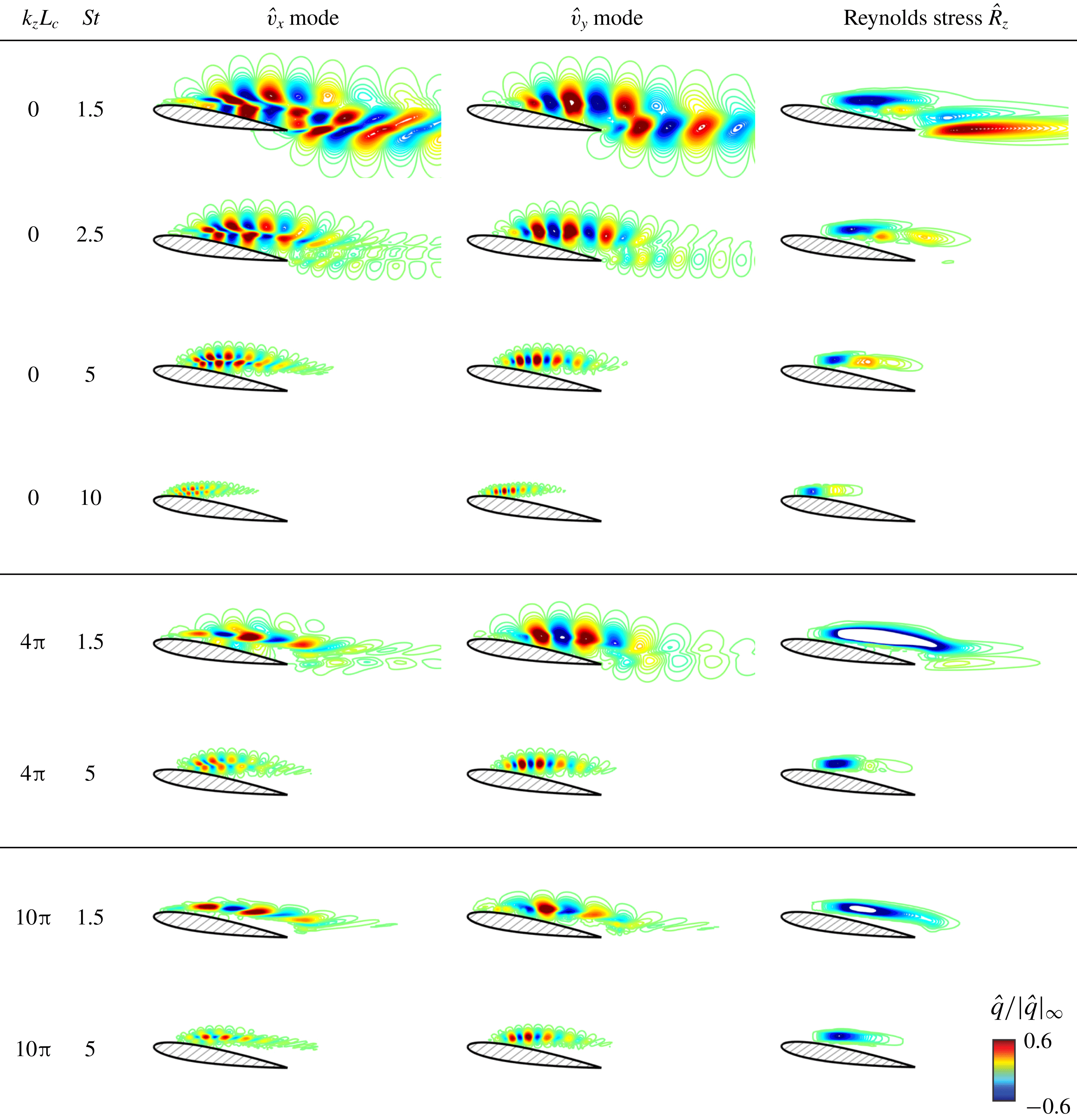
denotes the real component of the argument. We visualize the response modes in figure 11 in their streamwise velocity
 $\hat{v}_{x}$
, transverse velocity
 $\hat{v}_{y}$
and the associated spanwise Reynolds stress
 $\hat{R}_{z}$
with the representative
 $k_{z}L_{c}$
–
 $St$
combinations for the mean baseline flow at
 $\unicode[STIX]{x1D6FC}=9^{\circ }$
. For modes of
 $St=1.5$
and
 $2.5$
, response structure develops from the shear layer above the suction surface and extends farther into the wake. Particularly for
 $(k_{z}L_{c},St)=(0,1.5)$
, we observe an extended wake structure in the velocity modes as well as the resolvent Reynolds stress. The Reynolds stress exhibits a pattern of von Kármán vortex shedding with negative correlation developing in the shear layer above the airfoil and positive correlation extending from the trailing edge over the bottom. By increasing either
 $St$
or
 $k_{z}L_{c}$
, the streamwise extent of the modal structure reduces to the shear layer. Further increase of frequency moves the response structure towards the leading edge where the shear layer remains thin and is capable of supporting small-scale structures from high-frequency perturbations. In § 5, we will further explore the resolvent Reynolds stress and show that it provides insight into momentum mixing that is critical for suppressing stall. We will discuss a metric that incorporates the gain and the spatial integration of the resolvent Reynolds stresses to provide a quantitative guidance to separation control.
We have performed resolvent analysis for the mean baseline flows of
 $\unicode[STIX]{x1D6FC}=6^{\circ }$
and
 $9^{\circ }$
and discussed an extension to the standard approach for the two unstable linear operators. From the gain distribution over frequency and wavenumber, we have seen the shear-layer-dominated feature for the baseline flows at both angles of attack. In the next section, we discuss the results of controlled flows and investigate important flow physics that achieves suppression of separation. The enhancement in aerodynamic performances will later be compared to the prediction of resolvent analysis.
4 Large-eddy simulations of controlled flows
In this section, we examine open-loop separation control using the thermal actuator modelled by (2.1). To assess the effectiveness of flow control and to develop a database to relate the control effectiveness to resolvent analysis, we conduct a parametric study with LES over open-loop actuation frequency
 $St^{+}$
and wavenumber
 $k_{z}^{+}$
. We will start our discussion by giving an overall picture of how aerodynamic forces (lift and drag) respond to the chosen
 $St^{+}$
and
 $k_{z}^{+}$
. We then analyse the controlled flow fields to correlate the flow physics to the change in the aerodynamic forces and their fluctuation magnitudes. The near-field velocity profiles and surface pressure distributions are also investigated to reveal the mechanism of aerodynamic force modification. With the results obtained from LES, the control effects will be compared to the results of resolvent analysis in the next section.
For both angles of attack, we present the drag and lift coefficients respectively in figures 12 and 13 for controlled flows by sweeping through actuation frequencies and wavenumbers. Let us now direct our attention to the change in lift in figure 12. While the controlled lift data appear scattered for
 $\unicode[STIX]{x1D6FC}=6^{\circ }$
, the flow control for
 $\unicode[STIX]{x1D6FC}=9^{\circ }$
achieves enhancement in lift by up to
 $54\,\%$
with thermal-based actuation. On the right of both lift plots, we provide an additional scale of
 $\bar{C}_{L}/C_{L,0}$
with
 $C_{L,0}$
being the potential-flow lift for the baseline. We recall that, while the
 $\unicode[STIX]{x1D6FC}=9^{\circ }$
airfoil is in deep stall, the mildly separated baseline flow at
 $\unicode[STIX]{x1D6FC}=6^{\circ }$
reattaches and achieves
 $84\,\%$
of
 $C_{L,0}$
, leaving a smaller room for lift enhancement with active flow control. The lift enhancement at
 $\unicode[STIX]{x1D6FC}=6^{\circ }$
does not exhibit a clean trend as at
 $\unicode[STIX]{x1D6FC}=9^{\circ }$
, which is likely due to difference in the baseline
 $\bar{C}_{L}/C_{L,0}$
. However, for both angles of attack, the fluctuation in lift is generally reduced by over
 $85\,\%$
with active flow control, as shown in figure 14.
The time-averaged lift coefficients
 $\bar{C}_{L}$
of controlled flows for angles of attack of
 $\unicode[STIX]{x1D6FC}=6^{\circ }$
(a) and
 $\unicode[STIX]{x1D6FC}=9^{\circ }$
(b). In each plot, the black dashed line marks the baseline value for the corresponding angle of attack. The magenta dashed line marks the potential flow lift coefficient computed using the panel method.

The time-averaged drag coefficients
 $\bar{C}_{D}$
of controlled flows for
 $\unicode[STIX]{x1D6FC}=6^{\circ }$
(a) and
 $\unicode[STIX]{x1D6FC}=9^{\circ }$
(b). The black dashed line marks the baseline value for the corresponding angle of attack. Symbols are as in figure 12(a).

Root-mean-square of the lift coefficients
 $C_{L,rms}$
of controlled flow for
 $\unicode[STIX]{x1D6FC}=6^{\circ }$
(a) and
 $\unicode[STIX]{x1D6FC}=9^{\circ }$
(b). The black dashed line marks the baseline value for the corresponding angle of attack. Symbols are as in figure 12(a).

Drag for both angles of attack exhibits significant reduction with active flow control, as shown in figure 13. The thermal actuation achieves drag reduction of up to
 $45\,\%$
for
 $\unicode[STIX]{x1D6FC}=6^{\circ }$
and
 $49\,\%$
for
 $\unicode[STIX]{x1D6FC}=9^{\circ }$
. The corresponding reductions in the thrusting power evaluated by the same normalization in (2.2) are
 $0.284$
and
 $0.354$
respectively for
 $\unicode[STIX]{x1D6FC}=6^{\circ }$
and
 $\unicode[STIX]{x1D6FC}=9^{\circ }$
. Both values are larger than the deployed actuation power of
 $E^{+}=0.0902$
. More importantly, by comparing the drag reduction for both angles of attack, we observe that the effective range of the actuation frequency scales well with the chord-based actuation Strouhal number
 $St^{+}=\unicode[STIX]{x1D714}^{+}L_{c}/2\unicode[STIX]{x03C0}v_{\infty }$
. Significant drag reduction is achieved over
 $3\lesssim St^{+}\lesssim 15$
but a sharp loss in the drag reduction is observed at
 $St^{+}\approx 15$
for both
 $\unicode[STIX]{x1D6FC}=6^{\circ }$
and
 $9^{\circ }$
. For
 $St^{+}\gtrsim 15$
, no control case exhibits significant enhancement in aerodynamic forces. Similar to effective frequency range for drag reduction, the lift fluctuation shown in figure 14 is also observed to decrease significantly over
 $3\lesssim St^{+}\lesssim 15$
for both angles of attack. The frequency scaling with
 $St^{+}$
rather than the wake-based Fage–Johansen
 $St_{\unicode[STIX]{x1D6FC}}^{+}$
once again implies a shear-layer-dominated nature for separation control.
Another interesting feature in the change of aerodynamic forces is the distinct trend exhibited by the two-dimensional actuation (
 $k_{z}^{+}L_{c}=0$
) cases. We observe that drag, while still below the baseline value, increases near
 $St^{+}\approx 7.5$
for both angles of attack for
 $k_{z}^{+}L_{c}=0$
. When a spanwise variation (
 $k_{z}^{+}L_{c}>0$
) is introduced to the actuation profile, such increase in drag is absent from the intermediate range of actuation frequency. In fact, little difference can be observed in the change of aerodynamics forces with
 $k_{z}^{+}L_{c}=10\unicode[STIX]{x03C0}$
,
 $20\unicode[STIX]{x03C0}$
and
 $40\unicode[STIX]{x03C0}$
using the actuation power
 $E^{+}=0.0902$
in (2.2) for the present study.
Controlled flows for
 $\unicode[STIX]{x1D6FC}=6^{\circ }$
with
 $k_{z}^{+}L_{c}=0$
and the resolvent response modes (streamwise velocity
 $\hat{v}_{x}$
) at the corresponding
 $k_{z}$
–
 $St$
. The percentage change in the drag coefficient is computed using
 $\unicode[STIX]{x0394}\bar{C}_{D}=(\bar{C}_{D,control}-\bar{C}_{D,baseline})/\bar{C}_{D,baseline}$
and similarly for lift and lift-to-drag ratio. Note that the resolvent response modes are computed based on mean baseline flow. Iso-surface of
 $QL_{c}^{2}/v_{\infty }^{2}=50$
coloured by streamwise velocity is used in the flow visualization. The response modes are obtained with
 $t_{\unicode[STIX]{x1D6FD}}v_{\infty }/L_{c}=5$
and are shown by the contour lines of
 $\hat{v}_{x}/|\hat{v}_{x}|_{\infty }\in \pm [0.01,0.9]$
.

To reveal the cause for the distinctive trend in drag with
 $k_{z}^{+}L_{c}=0$
, we visualize the instantaneous flows for representative cases of
 $\unicode[STIX]{x1D6FC}=6^{\circ }$
in figure 15. Behind the
 $Q$
-criterion visualization, we also show the TKE contour as well as a black curve that marks
 $\bar{v}_{x}=0$
to indicate the separation region for each case. Along with the flow visualization, the percentage change of aerodynamic forces is tabulated on the left. In all cases, we find that thermal actuation is able to trigger the Kelvin–Helmholtz instability of the shear layer, exciting the roll-up and chopping the shear layer at the actuation frequency. Each chop forms a compact two-dimensional spanwise vortex, advecting along the suction side of the airfoil. These vortical structures promote momentum mixing and entrain the free stream. Similar to the discussion in Glezer et al. (Reference Glezer, Amitay and Honohan2005), the entrainment results in the Coandă-like effect and suppresses flow separation, which can be seen in cases 6-0A to 6-0D by comparing the
 $\bar{v}_{x}=0$
contours to that of the baseline. In what follows, we split the discussion into four ranges of frequencies according to the distinctive change in drag as well as similar flow responses to the actuation.
Frequency range:
 $0.6\lesssim St^{+}\lesssim 4.33$
(represented by cases 6-0A and 6-0B)
In this frequency range, the flow response is characterized by the coupling between the roll-up of the shear layer over the airfoil and the vortex shedding in the wake. Particularly for case 6-0B, we observe the formation of strong spanwise vortices that advect farther downstream into the wake, diminishing the development of three-dimensional structures and fully laminarizing the flow. The laminarization, however, leads to a decrease in lift which can also be inferred by the upward-deflected wake vortices shown in the flow visualization of 6-0B. Such a global laminarization is observed over
 $2\lesssim St^{+}\lesssim 4.33$
with two-dimensional actuation for
 $\unicode[STIX]{x1D6FC}=6^{\circ }$
. Although such flow laminarization is not observed in
 $0.6\lesssim St^{+}\lesssim 1.67$
, the coupling between the excited shear-layer roll-up and the wake shedding holds for this frequency range. Over the frequency range of
 $0.6\lesssim St^{+}\lesssim 4.33$
, the drag generally decreases with increasing actuation frequency.
Frequency range:
 $4.67\lesssim St^{+}\lesssim 7.33$
(represented by case 6-0C)
In this range, the pairing between the spanwise vortices takes place near the trailing edge. Though the flow is reattached before mid-chord due to actuation, the vortex pairing process results in trailing-edge separation and causes the drag to increase. The pairing process also stimulates the laminar–turbulent transition and increase TKE near the trailing edge, making the wake turbulent. The drag reaches the local maximum with
 $St^{+}\approx 7.33$
over the varied actuation frequency in this range.
Frequency range:
 $8\lesssim St^{+}\lesssim 11$
(represented by case 6-0D)
The flow response in this frequency range is characterized by the break-up of the spanwise vortices over the suction surface, accompanied by the laminar–turbulent transition before the pairing process takes place. It is also marked by the removal of the von Kármán shedding structures that are prominent in other regimes as well as the baseline. The break-up of the spanwise vortices occurs near the mid-chord with increased TKE, after which turbulent structures cover the rest of the suction surface. Compared to the baseline flow, these turbulent structures in case 6-0D possess higher streamwise momentum and advect close to the suction surface. The break-up process allows for three-dimensional mixing and keeps high-momentum turbulent structures staying adjacent to the suction surface, suppressing the trailing-edge separation. As a result, the drag further decreases and reaches the local minimum at case 6-0D with
 $St^{+}=11$
.
Frequency range:
 $St^{+}\gtrsim 11$
(represented by case 6-0E)
The drag increases beyond
 $St^{+}\gtrsim 11$
. In this range, the spanwise vortices are not sufficiently large and strong to induce enough momentum mixing for free-stream entrainment. By comparing the flow fields of 6-0E to that of the baseline, the appearance of the actuation-induced spanwise vortices is still visibly clear. However, while these smaller spanwise structures advect downstream, they also move away from the suction surface, as opposed to their trajectories in cases 6-0A to 6-0D. Even though the actuation still excites shear-layer roll-up, it does not effectively entrain the free-stream momentum and leads to the drag remaining at the baseline level near
 $St^{+}\approx 15$
.
Along with the above observations made from the controlled flows, we also examine the response modes from resolvent analysis in figure 15. We recall that these response modes are obtained from the resolvent analysis of the mean baseline flow. The response mode is provided at the frequency used for the unsteady actuation in each corresponding control case in the middle column. For case 6-0A and 6-0B, the corresponding response structure develops from the shear layer above the suction surface and extends farther into the wake. For higher frequencies, the streamwise extent of the modal structure reduces to the shear layer, starting from the mode at
 $St=7.33$
(case 6-0C) and for higher-frequency cases. According to these observations, we see that the response mode structure is capable of providing insights into the global flow receptivity to perturbation of specified frequency. When the modal structures cover both the shear layer and the wake, in corresponding controlled flows we observe that the perturbation amplified through the shear layer also advects into the wake and stimulates the shedding instability. Similarly, when the modal structures appear only within the shear layer, the corresponding controlled flow shows that the actuation-induced spanwise vortices either merge near the trailing edge or break up over the airfoil, never able to advect into the wake while remaining compact. Such a qualitative agreement between resolvent analysis and controlled flows has made it promising for resolvent analysis to provide quantitative design guidelines. We will further elaborate on this point in the next section.
Instantaneous flow fields and TKE (in the background) for the controlled cases with
 $k_{z}^{+}L_{c}>0$
of
 $\unicode[STIX]{x1D6FC}=6^{\circ }$
. Iso-surface of
 $QL_{c}^{2}/v_{\infty }^{2}=50$
coloured by streamwise velocity is utilized in the flow visualization.

Continuing the discussion for control cases at
 $\unicode[STIX]{x1D6FC}=6^{\circ }$
, we present the flow visualization for cases where a spanwise variation is introduced into the actuation with
 $k_{z}^{+}L_{c}>0$
in figure 16. We also refer to the drag value reported in figure 13(a) for the controlled cases. For all
 $k_{z}^{+}L_{c}>0$
examined, the drag decrease reaches
 $\bar{C}_{D}\approx 0.04$
at
 $St^{+}\approx 3$
and continues to maintain this level of approximately
 $40\,\%$
drag reduction from the baseline. The control effect degrades at
 $St^{+}\approx 10$
and returns to the baseline drag level by
 $St^{+}\approx 15$
. Similar to the
 $k_{z}^{+}L_{c}=0$
cases, the thermal actuation generates spanwise vortices near the leading edge, which can be seen in the flow visualization. These vortices carry the spanwise variation introduced by the actuation input for the actuation wavenumbers of
 $k_{z}^{+}L_{c}=10\unicode[STIX]{x03C0}$
,
 $20\unicode[STIX]{x03C0}$
and
 $40\unicode[STIX]{x03C0}$
(respectively corresponding to one, two and four waves across the spanwise extent in the current LES). These spanwise vortices advect along the suction surface and evolve into turbulent structures near mid-chord. Similar to the comments we made previously for case 6-0D on the effect of mid-chord transition, the same mechanism holds here for drag reduction in all effective cases with
 $k_{z}^{+}L_{c}>0$
. Therefore, as opposed to the controlled cases with
 $k_{z}^{+}L_{c}=0$
, drag reduction achieved from
 $k_{z}^{+}L_{c}>0$
remains at a comparable level over the intermediate actuation frequencies.
Analogous to the discussions of
 $\unicode[STIX]{x1D6FC}=6^{\circ }$
cases, we show representative control cases at
 $9^{\circ }$
with their flow visualizations in figure 17. A qualitative difference between the controlled flows of
 $\unicode[STIX]{x1D6FC}=9^{\circ }$
and those of
 $6^{\circ }$
is that the global laminarization by thermal actuation is not observed in any of the examined controlled cases with
 $k_{z}^{+}L_{c}=0$
for
 $\unicode[STIX]{x1D6FC}=9^{\circ }$
. Apart from these two differences, similar flow physics associated with the change in drag for
 $\unicode[STIX]{x1D6FC}=6^{\circ }$
also holds for the
 $\unicode[STIX]{x1D6FC}=9^{\circ }$
controlled cases. Cases 9-0A, 9-0B, 9-0C and 9-0D are respectively associated with four frequency ranges as discussed for
 $\unicode[STIX]{x1D6FC}=6^{\circ }$
with
 $k_{z}^{+}L_{c}=0$
in figure 15. In each frequency range, similar trend in the drag reduction is observed with the use of two-dimensional actuation in both
 $\unicode[STIX]{x1D6FC}=6^{\circ }$
and
 $9^{\circ }$
controlled cases. For
 $\unicode[STIX]{x1D6FC}=9^{\circ }$
, the partial laminarization of the flow by two-dimensional actuation is only observed over the suction surface in
 $5\lesssim St^{+}\lesssim 7.5$
. Along with drag reduction, significant lift enhancement from baseline flow of
 $\unicode[STIX]{x1D6FC}=9^{\circ }$
is also observed in cases where separation is effectively suppressed by thermal actuation. Suppression of separation can be attributed to the accelerated laminar–turbulent transition over separation bubble that occurs immediately after the shear-layer roll-up. In the case of
 $St^{+}=16$
, we observe that the small spanwise vortices depart from the suction surface and fail to suppress flow separation. As a consequence, the lift and drag returns to the baseline level at
 $St^{+}\approx 15$
. Qualitative agreement between the controlled flows and the resolvent response modes is also observed for the
 $\unicode[STIX]{x1D6FC}=9^{\circ }$
cases, similar to the the discussions for
 $\unicode[STIX]{x1D6FC}=6^{\circ }$
.
Instantaneous flow fields and TKE (in the background) for the baseline and controlled cases of
 $\unicode[STIX]{x1D6FC}=9^{\circ }$
. Iso-surface of
 $QL_{c}^{2}/v_{\infty }^{2}=50$
coloured by streamwise velocity is utilized in the flow visualization.

To provide further insights into the mechanism for suppressing flow separation, we examine three selective control cases from figure 17 along with the
 $\unicode[STIX]{x1D6FC}=9^{\circ }$
baseline in their near-field mean flows. The changes in the aerodynamics forces of these three control cases, 9-0B, 9-1B and 9-1C, are listed at the top of figure 18 with the baseline values for quick reference. Cases 9-0B and 9-1B employ the same actuation frequency (
 $St^{+}=5.5$
) but with different wavenumbers. While the levels of drag reduction are comparable for these two control cases, the introduction of spanwise-varying actuation in case 9-1B achieves further enhancement in lift compared to case 9-0B. Cases 9-1B and 9-1C both use
 $k_{z}^{+}L_{c}=10\unicode[STIX]{x03C0}$
but different
 $St^{+}$
. These two cases achieve comparable levels in lift enhancement and drag reduction across all drag data presented in figure 13.
Time- and spanwise-averaged streamwise velocity profiles over the airfoil (a) and in near wake at
 $x/L_{c}=2.0$
(b). Dashed curves mark the contours of
 $\bar{v}_{x}=0$
for the four cases.

For these three control cases, the time- and spanwise-averaged velocity profiles are provided over the airfoil and one chord downstream in the near wake (
 $x/L_{c}=2$
) in figure 18. Dashed curves are also shown in figure 18(a) to mark the contour of
 $\bar{v}_{x}=0$
for the comparison of separation region for the four cases. While the separation region covers the entire chord in the baseline flow, the periodically excited flow immediately reattaches after separation. In case 9-0B, the flow over the airfoil is laminarized with formation of compact spanwise vortices. These vortices merge near the trailing edge and the flow separates again near
 $x/L_{c}\approx 0.75$
. The occurrence of the trailing-edge separation can be envisioned from the increasing deficit in the streamwise velocity profiles observed farther upstream. We also observe in figure 17 that the spanwise vortices gradually depart from the suction surface as they advect downstream in case 9-0B. As opposed to case 9-0B, the accelerated transition by spanwise actuation in cases 9-1B and 9-1C provides further three-dimensional mixing and effectively entrains free-stream momentum, resulting in a fully attached boundary layer that extends to the trailing edge with
 $\boldsymbol{e}_{n}\boldsymbol{\cdot }\unicode[STIX]{x1D735}\bar{v}_{x}>0$
. Similar observations on the modification of velocity profiles have been made by Amitay & Glezer (Reference Amitay and Glezer2002) using actuation frequencies of
 $St^{+}\sim O(10)$
for separation control with synthetic jets. In cases 9-1B and 9-1C, the effective entrainment due to three-dimensional mixing further enhances the lift performance from that of case 9-0B. The wake profiles in figure 18(b) also provide insight into the drag reduction. All control cases exhibit reduced momentum deficit in the streamwise velocity profiles in their near wakes. In particular, we observe that the transverse locations where the wake profiles exhibit the maximum deficit move downwards in cases 9-1B and 9-1C. Such a transverse displacement suggests a stronger downwash and is reflecting the enhanced lift for cases 9-1B and 9-1C as well.
In figure 18(a), case 9-0B exhibits the smallest separated region. The two-dimensional actuation used in case 9-0B appears to reattach the flow more effectively than three-dimensional actuation. In spite of the earlier reattachment, case 9-0B provides the least suction over this separation region in
 $0\lesssim x/L_{c}\lesssim 2$
compared to cases 9-1B and 9-1C, as shown in figure 19(a). While all control cases provide higher suction than the baseline flow over this region, the use of three-dimensional actuation further enhances suction compared to two-dimensional actuation. As discussed for baseline flows, the laminar–turbulent transition occurs with a plateau in the pressure profile for the controlled cases also. Such a pressure plateau is clear in cases 9-1B and 9-1C. However, in case 9-0B where only laminar spanwise vortices are present, the airfoil does not benefit from the additional suction provided by the pressure plateau associated with laminar–turbulent transition.
Suction-surface pressure profiles (a) and their root-mean-square (b) of controlled flows and baseline for
 $\unicode[STIX]{x1D6FC}=9^{\circ }$
. Legends follow figure 18.

The shear-layer roll-up and transition processes can be identified from the pressure fluctuation profiles in figure 19(b). These two processes take place with the pressure fluctuation reaching the local maximum near
 $x/L_{c}\approx 0.21$
for cases 9-0B and 9-1B under the same actuation frequency of
 $St^{+}=5.5$
. With the higher
 $St^{+}$
in case 9-1C, the local maximum shifts upstream and suggests accelerated roll-up and transition processes. Through the discussion of the velocity and pressure profiles, we have noted that both the excited roll-up and laminar–turbulent transition processes are crucial for the suppression of separation. These mechanisms can encourage momentum mixing and entrain free-stream momentum to achieve flow reattachment, which provides enhanced aerodynamic performance.
Let us recapitulate our findings on the important flow physics for suppressing flow separation and the connection between those and the results from resolvent analysis. The mechanism for suppression of separation relies on enhanced momentum mixing. The mixing entrains free-stream momentum and can be provided by the excited roll-up of the shear layer over the suction surface as well as the laminar–turbulent transition process that follows the roll-up. As an observation from the study of controlled flows, the shear-layer-dominated physics for separation control aligns with the discussions in Greenblatt & Wygnanski (Reference Greenblatt and Wygnanski2000). Recalling that resolvent analysis also reveals the shear-layer-dominated energy amplification, capitalizing upon the shear-layer instability becomes critical for developing effective and efficient separation control techniques. In what follows, we leverage the knowledge of these flow physics and propose a resolvent-analysis-based guideline for the design of active separation control.
5 Assessment of control effect via resolvent analysis
We have performed resolvent analysis to reveal its insights into energy amplification over a range of frequencies and wavenumbers in § 3. The knowledge of amplification can be leveraged for flow control, since highly amplified perturbations may change the mean flow through nonlinear effects. By comparing the controlled flows to the resolvent response modes, we found that the modal structures provide insights into the global receptivity to a specified perturbation. We have also learned from controlled flows that momentum mixing over the airfoil plays an important role in suppressing separation in § 4. The enhancement of aerodynamic performance can be quantified by the momentum mixing taking place over the airfoil. This section takes the insights from the resolvent analysis and the LES of controlled flows to provide quantitative guidelines for the design of unsteady separation control.
While resolvent response modes can capture coherent structures, mixing provided by these coherent structures can be examined through the Reynolds stress associated with the mode (Luhar, Sharma & McKeon Reference Luhar, Sharma and McKeon2014, Reference Luhar, Sharma and McKeon2015). We have also noted that the location of momentum mixing is crucial to modify the base state and alter the aerodynamic performance. Over the airfoil, the roll-up and transition processes enhance mixing and suppress flow separation. On the other hand, momentum mixing induced by large-scale von Kármán structure in the wake widens the wake and results in increased streamwise momentum deficit and higher drag. Such mixing is thus unfavourable for aerodynamic stall control. To address the different effects of these two kinds of mixing, we discuss four representative controlled cases along with the resolvent Reynolds stress obtained from the mean baseline flow for the corresponding
 $k_{z}L_{c}$
–
 $St$
in figure 20. For the case with
 $(k_{z}^{+}L_{c},St^{+})=(0,1)$
, we observe an extended wake structure in the Reynolds stress with a strong vortex-shedding pattern, causing unfavourable mixing for drag reduction. Such mixing in the wake is absent in the other three wavenumber–frequency combinations. Correspondingly, the use of
 $(k_{z}^{+}L_{c},St^{+})=(0,1.5)$
results in lower performance enhancement compared to the other three controlled cases, particularly in drag. Therefore, for aerodynamically favourable control, we should leverage mixing that takes place over the airfoil by considering the resolvent Reynolds stress as a possible metric for guidance.
Comparison of the enhancement in
 $\bar{C}_{L}$
and
 $\bar{C}_{D}$
and the spanwise Reynolds stress of resolvent response mode for the corresponding
 $k_{z}L_{c}$
and
 $St$
. Note that the resolvent response modes are computed based on mean baseline flow. The response modes are obtained with
 $t_{\unicode[STIX]{x1D6FD}}v_{\infty }/L_{c}=5$
and the associated
 $\hat{R}_{z}$
are visualized by the contour lines of
 $\hat{R}_{z}/|\hat{R}_{z}|_{\infty }\in \pm [0.01,0.9]$
.

The momentum mixing associated with resolvent response mode can be characterized through performing a spatial integral of the corresponding Reynolds stresses over a region of physical interest (Nakashima, Fukagata & Luhar Reference Nakashima, Fukagata and Luhar2017). Here, we quantitatively assess mixing by introducing a spatial window to perform integration of resolvent Reynolds stress. We choose a window that covers the shear layer over the airfoil so that only the mixing taking place in this crucial region for suppression of separation is taken into account. This window
 $w(\boldsymbol{x})$
, shown in figure 21, is designed as a level-set function with
 $\int _{\unicode[STIX]{x1D6FA}}w(\boldsymbol{x})\,\text{d}\boldsymbol{x}=1$
. This level-set function is obtained by evaluating
 $|\hat{v}_{x}^{\ast }\hat{v}_{y}|$
for the dominant shear-layer eigenmode shown in figure 6. In appendix C, we also demonstrate that the present assessment is robust with respect to the choice of the window. The spatial integration for modal Reynolds stress considers
 $w(\boldsymbol{x})$
as a weighting function and is performed over the entire domain
 $\unicode[STIX]{x1D6FA}$
as
 $$\begin{eqnarray}\displaystyle M(k_{z},\unicode[STIX]{x1D714})\equiv \int _{\unicode[STIX]{x1D6FA}}[\unicode[STIX]{x1D70E}_{1}^{2}(\hat{R}_{x}^{2}+\hat{R}_{y}^{2}+\hat{R}_{z}^{2})^{1/2}]_{k_{z},\unicode[STIX]{x1D714}}w(\boldsymbol{x})\,\text{d}\boldsymbol{x}, & & \displaystyle\end{eqnarray}$$
where we also associate the gain
 $\unicode[STIX]{x1D70E}_{1}$
in the integration considering the amplification from a unit energy of forcing. With this scalar function
 $M(k_{z},\unicode[STIX]{x1D714})$
, the mixing that is favourable for flow control can be evaluated by the integrated Reynolds stresses from the resolvent response mode at
 $k_{z}$
–
 $\unicode[STIX]{x1D714}$
.
Spatial integration of the modal Reynolds stress,
 $M(k_{z},\unicode[STIX]{x1D714})$
, for
 $k_{z}L_{c}=0$
,
 $10\unicode[STIX]{x03C0}$
,
 $20\unicode[STIX]{x03C0}$
and
 $40\unicode[STIX]{x03C0}$
for (a)
 $\unicode[STIX]{x1D6FC}=6^{\circ }$
and (b)
 $\unicode[STIX]{x1D6FC}=9^{\circ }$
airfoils. Over the airfoil, the shear-layer window represented by the level-set function in the lower-left corner is used as the weight in the spatial integration performed in (5.1).

We show the integrated resolvent Reynolds stress
 $M(k_{z},\unicode[STIX]{x1D714})$
using the shear-layer windows in figure 21. The trend in
 $M(k_{z},\unicode[STIX]{x1D714})$
suggests higher mixing is achieved by resolvent response modes over the shear layer near
 $St\approx 5$
and low
 $k_{z}L_{c}$
for both angles of attack. With the mixing quantified by
 $M(k_{z},\unicode[STIX]{x1D714})$
for resolvent response modes, we colour the data points of aerodynamic forces from controlled cases by the corresponding
 $M(k_{z}^{+},\unicode[STIX]{x1D714}^{+})$
for both angles of attack in figure 22. In both figures, we show time-average drag, lift and lift-to-drag ratio with the level of modal mixing
 $M(k_{z}^{+},\unicode[STIX]{x1D714}^{+})$
. We observe that the drag reduction and lift enhancement achieved by active flow control correlate well with the level of mixing based on
 $M(k_{z}^{+},\unicode[STIX]{x1D714}^{+})$
from resolvent analysis of the mean baseline flow. Over the actuation frequency range of
 $3\lesssim St^{+}\lesssim 12$
, where most of the effective control cases reside, successful control is characterized by high levels of shear-layer mixing over the airfoil according to resolvent analysis. Particularly for the lift data of
 $\unicode[STIX]{x1D6FC}=9^{\circ }$
, the maximum lift agrees well with the high value of
 $M$
. Similarly for
 $\unicode[STIX]{x1D6FC}=9^{\circ }$
, the sluggish decrease in drag over the low-frequency range can also be related to the mixing that takes place in the wake for low-frequency modes, as discussed in figure 20. At this stage, we have observed both qualitative and quantitative agreements between resolvent analysis and controlled flows obtained from LES. The positive correlation between the enhancement of aerodynamic performance and the modal mixing from resolvent analysis suggests its capability of serving as a guiding tool towards selecting effective actuation parameters.
Relative change in the time-average drag, lift and lift-to-drag ratio coloured by the corresponding
 $M(k_{z}^{+},\unicode[STIX]{x1D714}^{+})$
for
 $\unicode[STIX]{x1D6FC}=6^{\circ }$
(a–c) and
 $\unicode[STIX]{x1D6FC}=9^{\circ }$
(d–f). The change in the drag coefficient is computed using
 $\unicode[STIX]{x0394}\bar{C}_{D}=(\bar{C}_{D,control}-\bar{C}_{D,baseline})/\bar{C}_{D,baseline}$
and similarly for lift and lift-to-drag ratio. In each plot, the dashed line corresponds to the baseline level. Symbols represent different actuation wavenumbers. ○:
 $k_{z}^{+}L_{c}=0$
;▵:
 $k_{z}^{+}L_{c}=10\unicode[STIX]{x03C0}$
; ♢:
 $k_{z}^{+}L_{c}=20\unicode[STIX]{x03C0}$
; ▿:
 $k_{z}^{+}L_{c}=40\unicode[STIX]{x03C0}$
.

The nonlinear physics beyond resolvent analysis
With resolvent analysis being a linear technique for the present nonlinear fluid-flow problem, we also observed some limitations of the interpretation in the aerodynamic performance and the prediction of
 $M(k_{z}^{+},\unicode[STIX]{x1D714}^{+})$
. Below, we comment on these limitations and identify the associated nonlinear physics.
For controlled cases with
 $k_{z}^{+}L_{c}=0$
, drag increases over
 $4\lesssim St^{+}\lesssim 10$
for both angles of attack. Such increase in drag is not captured by the value of
 $M$
. As discussed in the previous section, this drag increase is due to the vortex merging process that causes trailing-edge separation. Therefore, the difference between the controlled flow results and resolvent analysis can be attributed to the nonlinear nature of the merging process that transfers energy from a fundamental frequency to its subharmonics. With the energy transfer across frequency space, this nonlinear process is not captured by the linear resolvent analysis that deals with a harmonic input–output process.
Another nonlinear process that leads to differences between the LES findings and the results of resolvent analysis is the laminar–turbulent transition following the break-up of spanwise vortices. In the previous section, the transition process has been shown to be a mechanism responsible for the suppression of separation, in addition to the shear-layer excitation. Such a mechanism is particularly important for suppressing stall in the control cases with high frequency near
 $St^{+}\approx 10$
and
 $k_{z}^{+}L_{c}>0$
, leading to peak drag reduction at
 $St^{+}\approx 12$
for
 $\unicode[STIX]{x1D6FC}=9^{\circ }$
and comparable level of force enhancement across three choices of three-dimensional actuation profiles (
 $k_{z}^{+}L_{c}>0$
). However, the level of
 $M(k_{z},\unicode[STIX]{x1D714})$
evaluated from resolvent analysis suggests degraded mixing for
 $k_{z}L_{c}>0$
and high frequencies. Therefore, while the aerodynamic forces benefit from the laminar–turbulent transition, this nonlinear process is also beyond the capability of resolvent analysis to predict the force enhancement through transition by using the quantitative level of
 $M(k_{z},\unicode[STIX]{x1D714})$
.
Resolvent analysis as a guiding tool for separation control
We have presented a design guideline that leverages the knowledge obtained from resolvent analyses performed on mean baseline flows for suppressing stall. We evaluate the level of mode-based mixing by combining the knowledge of amplification, modal structure and a shear-layer window over the airfoil, providing a scalar function over the frequency–wavenumber space. In spite of slight deviations due to the nonlinear physics beyond the present linear modal, the control effect well correlates with lift enhancement and drag reduction for open-loop controlled flows. Such a guideline provides quantitative assessment towards selecting actuation frequency and wavenumber for effective unsteady separation control.
6 Conclusion
We presented an active flow control effort that capitalizes on the resolvent analysis of the separated flows over a NACA 0012 airfoil at angles of attack of
 $\unicode[STIX]{x1D6FC}=6^{\circ }$
and
 $9^{\circ }$
and a chord-based Reynolds number of
 $23\,000$
. The objective of our study was to provide design guidelines for separation control by leveraging the insights gained from resolvent analysis of mean turbulent flows. The guideline was tested against a large number of LES cases with flow control implemented.
The resolvent analysis started by extracting the linear Navier–Stokes operator that governs the perturbations about the statistically stationary turbulent mean flows obtained from the baseline LES. In the present analysis, the nonlinearity is retained by treating it as an internal forcing in the formulation. To analyse the unstable linear operators (base states), we considered an extension to the standard approach of resolvent analysis by introducing a temporal filter such that the input–output analysis is performed over a finite-time horizon. We observed the gain as well as the modal structure physically correlate with the time constant of the temporal filter. By sweeping through the Fourier space spanned by the frequency and spanwise wavenumber, we observed that the gain distribution scales well with the chord-based Strouhal number between both angles of attack. This scaling behaviour stems from the high non-normality of the shear-layer modes in the operator spectrum that expands the pseudospectral radius. Based on these findings, the resolvent analysis revealed a shear-layer-dominated mechanism for energy amplification from the input–output process.
The LES of controlled flows were performed with a thermal actuator that introduces time-periodic heat injection with a prescribed spanwise profile. We swept through different choices of actuation frequency and spanwise wavenumbers to investigate their effects on suppressing stall and enhancing the aerodynamic performance. In successful controlled cases, the periodic thermal actuation reduces drag by up to
 $49\,\%$
and enhances lift by up to
 $54\,\%$
. The fluctuation in lift is also reduced by up to
 $85\,\%$
. According to the trend of drag reduction over frequencies, we once again observed that the effective frequency for both angles of attack scales well with the chord-based Strouhal number. Aligning with the literature are the observations on the shear-layer-dominated physics in suppressing separation. We also examined the control cases in their flow fields and the associated change in the aerodynamic forces. With the examination, we concluded that the excitation of shear-layer roll-up and the subsequent laminar–turbulent transition are two critical mechanisms in enhancing momentum mixing to entrain the free-stream momentum. Both mechanisms contribute to the enhancement of aerodynamic performances by reducing drag and increasing lift.
The study of controlled flows showed that mixing over the suction surface plays a key role suppressing separation. As such, we evaluated mixing provided by resolvent response modes obtained from mean baseline flows. We quantified the modal mixing by integrating the Reynolds stresses associated with the response mode over a shear-layer window. By comparing the modal mixing to the force data obtained from LES, we observed good correlation between the higher modal mixing and enhanced control effects for both angles of attack. Such quantitative agreement assures the utility of resolvent analysis for selecting effective actuation frequencies and wavenumbers, even when the analysis is performed on the mean baseline flow. Although slight deviations are found in such a correlation, they can be attributed to the nonlinear physics such as vortex merging and laminar–turbulent transition. These nonlinear processes are beyond the validity of the linear input–output process captured through resolvent analysis.
Through this effort, we have demonstrated that resolvent analysis is a valuable tool for providing physics-based guideline for designing separation control. Such a guideline gives insights into the effective actuation frequencies and wavenumbers for separation control with periodic actuation. The present analysis was performed on the mean baseline flow to serve as a predictive tool for the choices of actuation frequencies and wavenumbers. It also provides quantitative support for the shear-layer-dominated physics for separation control. Note that the present approach can also serve as a basis to design a closed-loop controller with appropriate sensors and actuators. We believe that this study can provide insights for the use of resolvent analysis in guiding future implementation of active flow control.
Acknowledgements
The authors acknowledge the US Office of Naval Research (N00014-16-1-2443, managed by Dr K. Iwanski) and Army Research Office (W911NF-14-1-0224, managed by Dr M. Munson) for supporting this study. We also thank Professor P. Schmid and Professor M. Jovanović for insightful discussions on the use of discounted resolvent analysis. We also acknowledge Dr Y. Sun for her help with code development and continuous feedback on this study. The computations were supported by the High Performance Computing Modernization Program at the US Department of Defense and the Research Computing Center at Florida State University. We also thank Ms O. Murray for her help in facilitating the extensive computations in this study.
Appendix A. Convergence of resolvent norm
We document the grid convergence with respect to the resolvent norm in table 2, in which the size of the domain and the grid resolution in both near and far field of the
 $\unicode[STIX]{x1D6FC}=9^{\circ }$
airfoil are investigated. We examine the convergence of the leading (
 $\unicode[STIX]{x1D70E}_{1}$
) and second (
 $\unicode[STIX]{x1D70E}_{2}$
) singular values of discounted resolvent operator (3.21) using
 $t_{\unicode[STIX]{x1D6FD}}v_{\infty }/L_{c}=5$
,
 $k_{z}L_{c}=0$
and
 $St=5.5$
, as the gain distribution reaches its maximum at the chosen frequency. Mesh
 $\mathbf{E}$
is chosen for this study with six-digit convergence in the leading singular value.
The modal mixing function
 $M(k_{z},\unicode[STIX]{x1D714})$
computed under different choices of
 $t_{\unicode[STIX]{x1D6FD}}$
evaluated for (a)
 $k_{z}L_{c}=0$
and (b)
 $k_{z}L_{c}=10\unicode[STIX]{x03C0}$
.

Grid convergence with respect to the singular values (
 $\unicode[STIX]{x1D70E}_{1}$
and
 $\unicode[STIX]{x1D70E}_{2}$
) of
 $\unicode[STIX]{x1D643}_{\bar{\boldsymbol{q}},\unicode[STIX]{x1D6FD}}$
with
 $t_{\unicode[STIX]{x1D6FD}}v_{\infty }/L_{c}=5$
,
 $k_{z}L_{c}=0$
and
 $St=5.5$
. Parameter
 $N_{s}$
denotes the number of points on the suction surface of the airfoil and
 $N_{total}$
denotes the total number of points of the mesh. Mesh
 $\mathbf{E}$
is chosen to conduct the analyses in this work.

Appendix B. On the choice of
$t_{\unicode[STIX]{x1D6FD}}$

Since the control effect was assessed according to the modal mixing function
 $M(k_{z},\unicode[STIX]{x1D714})$
, we show the robustness of the assessment with respect to different choices of the discounting time parameter,
 $t_{\unicode[STIX]{x1D6FD}}$
, by their corresponding
 $M(k_{z},\unicode[STIX]{x1D714})$
in figure 23. We show representative wavenumbers of
 $k_{z}L_{c}=0$
and
 $10\unicode[STIX]{x03C0}$
, with
 $t_{\unicode[STIX]{x1D6FD}}$
decreasing from
 $t_{\unicode[STIX]{x1D6FD}}v_{\infty }/L_{c}=7$
to 1. We note that all choices reveal both shear-layer and wake structures in their response modes, as shown in figure 9. Moreover, the trend of
 $M(k_{z},\unicode[STIX]{x1D714})$
over the spectral space remains effectively unchanged regardless of the different choices of
 $t_{\unicode[STIX]{x1D6FD}}$
. As the assessment of separation control effect is built upon the trend of
 $M(k_{z},\unicode[STIX]{x1D714})$
, we conclude that the present approach is robust against the choice of
 $t_{\unicode[STIX]{x1D6FD}}$
as long as the shear-layer and wake structures can be revealed with the chosen
 $t_{\unicode[STIX]{x1D6FD}}$
.
Appendix C. Window of integration on resolvent Reynolds stress
Relative change in the time-average drag, lift and lift-to-drag ratio coloured by the corresponding
 $M^{\prime }(k_{z}^{+},\unicode[STIX]{x1D714}^{+})$
for
 $\unicode[STIX]{x1D6FC}=6^{\circ }$
(a–c) and
 $\unicode[STIX]{x1D6FC}=9^{\circ }$
(d–f). The change in the drag coefficient is computed using
 $\unicode[STIX]{x0394}\bar{C}_{D}=(\bar{C}_{D,control}-\bar{C}_{D,baseline})/\bar{C}_{D,baseline}$
and similarly for lift and lift-to-drag ratio. In each plot, the dashed line corresponds to the baseline level. Symbols represent different actuation wavenumbers. ○:
 $k_{z}^{+}L_{c}=0$
;▵:
 $k_{z}^{+}L_{c}=10\unicode[STIX]{x03C0}$
; ♢:
 $k_{z}^{+}L_{c}=20\unicode[STIX]{x03C0}$
; ▿:
 $k_{z}^{+}L_{c}=40\unicode[STIX]{x03C0}$
.

The integration of Reynolds stress in (5.1) involves a spatial window over which the integration is performed. Here, we examine another choice for this window in its effect on the quantitative correlation discussed in figure 22. Instead of providing a level-set function according to the dominant shear-layer eigenmode, we can integrate the Reynolds stress associated with the response mode over the domain above the airfoil as
 $$\begin{eqnarray}\displaystyle M^{\prime }(k_{z},\unicode[STIX]{x1D714})\equiv \int _{x_{LE}}^{x_{TE}}\int _{y_{s}(x)}^{+\infty }[\unicode[STIX]{x1D70E}_{1}^{2}(\hat{R}_{x}^{2}+\hat{R}_{y}^{2}+\hat{R}_{z}^{2})^{1/2}]_{k_{z},\unicode[STIX]{x1D714}}\,\text{d}y\,\text{d}x, & & \displaystyle\end{eqnarray}$$
where
 $y_{s}(x)$
denotes the profile of the suction surface as a function of
 $x$
, and
 $x_{LE}$
and
 $x_{TE}$
respectively denote the streamwise locations of leading and trailing edges. Using this scalar function
 $M^{\prime }(k_{z},\unicode[STIX]{x1D714})$
to quantify modal mixing, we generate similar plots in figure 24 and compare it to figure 22. We observe that the use of the new window in equation (C 1) provides the same conclusive assessment with the positive correlation between the level of
 $M^{\prime }(k_{z},\unicode[STIX]{x1D714})$
and the performance enhancement. This suggests the developed guideline is robust in the choice of the integration window as long as the window reasonably highlights the shear layer over the suction surface.