I. INTRODUCTION
The efficiency η of a thermogenerator (TEG) is commonly defined as the net electrical power output, – P, divided by the thermal power Q h supplied, whereas the coefficient of performance (COP) ≡ φ of a Peltier cooler (TEC) is defined as the ratio of the cold side cooling power (Q c) by the electrical power (P) supplied:

Global maximization of these performance parameters is a suitable guideline for an empirical approach to thermoelectric (TE) device optimization. Nevertheless, it is more attractive for optimization purposes to express both η and φ in terms of the intensive variables as are relative current density u and reduced “efficiencies” η r and φ r that are used as primary values within the framework of the compatibility approachReference Snyder and Ursell1; for an overview see also Refs. Reference Ursell and Snyder:2–Reference Seifert, Zabrocki, Snyder and Müller5.
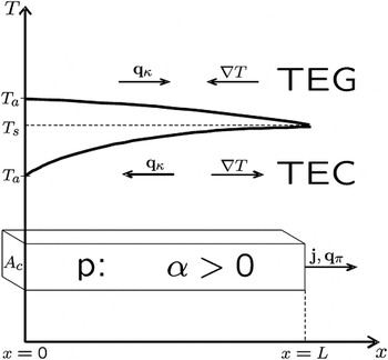
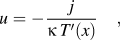
In this paper, we use the notation for a unified model of TEG/TEC under steady-state conditions introduced in Refs. Reference Seifert, Zabrocki, Snyder and Müller5 and Reference Seifert, Müller and Walczak6, where the absorbing side denoted with index “a” in a generator is the hot side (index “h”) and in a cooler is the cold side (index “c”). For the sink side denoted with the index “s” it is vice versa. In particular, we refer to a prismatic TE element of length L, cross-sectional area A c, and fixed boundary temperatures T a and T s (see Fig. 1), where T a is the temperature at the heat absorbing side (T a = T h for TEG, but T a = T c for TEC), and T s denotes the heat sink temperature that is often fixed to the room temperature. Assuming parallelity of heat flux and electrical current density (flow direction x axis), we end up in a one-dimensional description, where the relative current density is defined as
Unified one-dimensional model of a TE element (single p-type pellet of length L, constant cross-sectional area A c): Cooling operation (TEC case) with T a < T s; TE generator (TEG case; T a > T s; smaller bowing due to relatively lower current compared to the TEC). Vector flows are indicated by the symbols q = – κ ∇T + α T j =: qκ + qπ with thermal and Peltier heat flux qκ and qπ, respectively (see Ref. Reference Seifert, Müller, Walczak and Rogl4). Note that T(x) peaks in the interior of the TE element only above the optimum current j = j opt for maximum efficiency and maximum COP, respectively. This can be shown exactly in the case of constant material properties.

with j = I/A c being the electrical current density.
II. REDUCED EFFICIENCIES AND COMPATIBILITY FACTORS FOR TEG AND TEC
Considering the COP of a TEC first, we find within the framework of the constant properties model

with Seebeck coefficient α, resistivity ρ = 1/σ, isothermal electrical conductivity σ, and thermal conductivity κ (under zero current). Taking the limits for an infinitesimal segment ( , etc.), we obtain

with j/u = – κT′(x), z = α 2σ/κ and uα/z = – jρ/[αT′(x)] we finally get

where φ r is the reduced COP.
An equivalent derivative can be found for the local efficiency (see Ref. Reference Snyder and Rowe3, section 9.2.2.)

whereby ∆T = T a – T s must be defined positive to get a positive Carnot factor for TEG. Note that the relative current density u is different for TEG and TEC, because u contains the temperature gradient primarily. As a consequence we find for better materials (higher zT) increasing contributions η loc and φ loc to the total performance. Thus, if a material is good, then it is for both applications.
Further note that TEG and TEC cases are only distinguished by the sign of u(T) if the same (temperature dependent) material properties, the same current density, but reversed boundary temperatures T a and T s are applied (T a > T s for TEG, but T a < T s is usual for TEC). For this case of directly comparing TEG and TEC we find formally η r = 1/φ r. This is ultimately a consequence of the underlying TE effects that are inverse to each other. Finally, the reduced “efficiencies” η r and φ r can be considered as local and irreversible representatives of the appropriate global performance parameters:

and

The reduced efficiencies present local maxima for u = s, where s is the compatibility factor
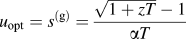
of a TEG, but

of a TEC, first introduced by Snyder and Ursell.Reference Snyder and Ursell1, Reference Ursell and Snyder:2 Note that the compatibility factors are, like z, temperature dependent material properties derived from the temperature dependent α, κ, and σ.
III. PERFORMANCE OF A SELF-COMPATIBLE ELEMENT
The total performance (efficiency and COP, respectively) of a finite element is obtained by summing up all local contributions (with a weighting factor 1/T) all over a TEG or TEC element in an integral sense as proposed by Harman and HonigReference Harman and Honig7; see also Ref. Reference Seifert, Müller, Walczak and Rogl4:
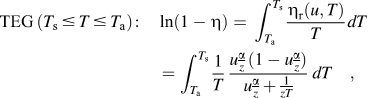
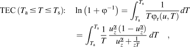
where we identify one kernel for integrals of both generator and cooler.
The integrals (6) can be optimized with respect to the relative current u: an optimized u represents an optimal ratio between heat flux and electrical current density and hence a maximum performance value given by the compatibility factors s = u opt; the theoretical background is the calculus of variations.Reference Seifert, Zabrocki, Snyder and Müller5 Such TE elements are called self-compatible elements.
If we assume the ability to achieve full self-compatibility (considering the case of infinite staging), we can apply u = s (g) and u = s (c) to the integrals (6), respectively, so that they take their maximal values with the optimal reduced efficiency

for both TEG and TEC.Reference Ioffe8, Reference Sherman, Heikes and Ure9 Then fully self-compatible performance parameters η sc and φ sc are given by
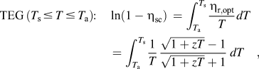
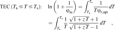
which is equivalent to Sherman’sReference Sherman, Heikes and Ure9 notation
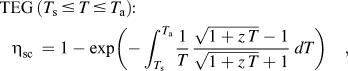
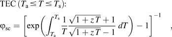
where integration is counted from the cold side to the hot side in both cases.
One of the major objectives in research on functionally graded materials (FGM) is to find optimal graded TE elements to achieve maximum performance. However, because both z T and s depend on the same materials parameters, a compromise between high z T and self-compatibility will need to be reached for true optimization under the constraint of a limited variability of the interrelation of the TE properties α, σ, and κ among the available real materials. On this account, u = s can only be fulfilled approximately in practice.
IV. THE CONSTRAINT z T = const
An optimization strategy related to graded material properties requires constraints, for instance, a limit for the figure of merit z(T)T. As an example, we consider here the particular case zT = const., which is easy to handle.
Analytical expressions of the integrals (8) can be found for z = const. as well as for zT = ko = const.; in the latter case we have with constant values 
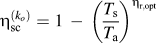
for TEG, and
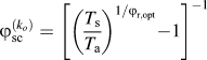
for TEC. A summary of all integral approximations is presented in the appendix of Ref. Reference Seifert, Zabrocki, Snyder and Müller5.
A central question is to enlighten the interrelation between the maximum performance expressions given by Eqs. (8) and (9). We initially emphasize that there is no extremal value task for the z T value. This can be shown by considering the integrals in Eq. (8),
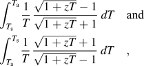
where we identify expressions being monotonous with z T in the integrands. Let us assume that z = z(T), then the integrals give different results for different functions z = z(T). This can be substantiated mathematically: the respective equations
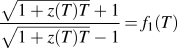
and
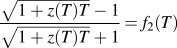
can easily be solved for z(T). Thus, an arbitrary function f 1(T) > 1 in the first case or 0 < f 2(T) < 1 in the second case can be generated with an appropriate z(T). Then, the first integral is bounded above by ln(T a/T s), whereas the second integral gives an arbitrary result greater then ln(T s/T a).
The question of how to get the best performance can only be answered if we put the constant ko in relation to the TE material. Proof is given in the Appendix that

if ko is calculated as the average over temperature [see Eq. (A3)] of a monotonously increasing function z(T)T; see also Eqs. (A7) and (A8) in Remark 2 of the Appendix. Obviously, this is a stricter approximation than identifying ko with a local maximum of z(T) T or z(T) To with a fixed temperature To. Often zT m is used with T m = (T a + T s)/2; see e.g., the Ioffe efficiency formula.
V. OPTIMAL TE POTENTIAL AND THE CONSTRAINT z T= const
It is necessary for any materials’ optimization to take full advantage of the potentialities of the TE material. Using the compatibility approach, Snyder and coworkersReference Snyder and Ursell1–Reference Snyder and Rowe3, Reference Snyder10, Reference Snyder11 derived two primary control parameters: the relative current u and the TE potential Φ, where Φ can simply be derived from the total heat flux, assuming parallelity of electrical current and heat flux:
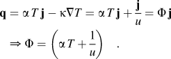
Snyder and UrsellReference Snyder and Ursell1, Reference Snyder and Rowe3 pointed out that the efficiency η is then simply given by the relative change of the TE potential; an analogous relation can be found for the COP (see Ref. Reference Seifert, Müller, Walczak and Rogl4):

This result points to the importance of the TE potential as a function of state: integrating the local efficiencies becomes simply a function of the TE potential at the two ends of the TE process.
Applying u = s, the equivalent optimal TE potential is given by

where the minus sign applies for TEG, but the plus sign applies for TEC. We further find
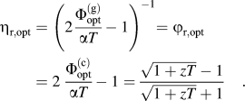
Using Eqs. (9), (12), and (13) and comparing with the Carnot efficiency of both TEG and TEC,
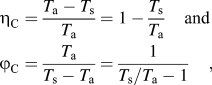
respectively, we finally get (if zT = const.)


Depending on the boundary conditions, the inequalities (15) measure the distance to reversibility for both TEG and TEC. Note that reversibility is only reached if  followed by
 . Because heat conduction is part of physics in available TE materials, even self-compatible elements operate far from Carnot, as in this numerical example:


Two further conclusions can be drawn from Eqs. (15) in this compact form. A comparison of the terms shows that the optimal Seebeck profile is increasing from the heat absorbing side to the heat sink side of the TE element; that is, we have α s > α a for both TEG and TEC. Moreover, the temperature dependence of the optimal Seebeck coefficient α(T) is found to be
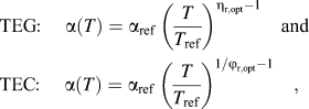
where α ref = α(T ref). Note that this result can also be derived from the differential equation for u(T) (see Ref. Reference Snyder and Ursell1)
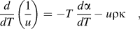
if u = s is applied together with the constraint zT = const. For details we refer to Ref. Reference Müller, Zabrocki, Goupil, Snyder, Seifert and Rowe12.
VI. DISCUSSION
Performance of fully self-compatible TE elements has been discussed in relation to the average value and temperature characteristics of the dimensionless figure of merit. In the performance integrals, z(T)T is representing an internal degree of freedom in scaling their value that must be fixed by an upper limit or similar constraint. In this context, the constraint zT = const. is particularly relevant: although important and often used in practice, it may not be realistic with available materials. Without a doubt, it is a challenge to combine real, temperature dependent material profiles α(T), σ(T), and κ(T) in a way that z(T)T = Tα 2(T)σ(T)/κ(T) = ko = const.; usually this can only be reached approximately. This leads to a specific answer to the question of a physically justified reference of an “equally good” TE material: proof is given in this paper that, if ko is identified with the average over z(T) T, formulae (9) serve as upper bounds for maximum performance in comparison to performance values calculated from Eq. (8). This holds true as long as the product z(T)T is monotonically increasing with temperature; this condition is fulfilled in most cases when chemically homogeneous materials are used in practical applications. Note that the performance may increase more for falling z(T)T curves; apart from the fact that no upper limit can be found, this region is practically not usable for most materials. In all cases, the degree or mismatch in self-compatibility has to be checked when using experimentally measured material properties.
Furthermore, it has been shown that the compatibility approach together with the introduction of the TE potential opens up a new option for analytical treatment when optimizing the performance of TE elements and devices. The use of self-compatible elements that represent an optimal match of the thermal and electric impedance locally, based on the local criterion u = s, provides an ultimate condition to completely exploit the potentiality of the material given by the figure of merit zT. Such elements are characterized by an optimal combination of material profiles where the optimal Seebeck profile α(T), when derived from the constraint z(T)T = ko = const., is given by a simple relation [see Eq. (16) for TEG and TEC].
A related work by Bian and coworkersReference Bian, Wang, Zhou and Shakouri13 uses a different method to improve performance. Although they do not explicitly invoke the compatibility factor, their method improves self-compatibility and therefore performance: an optimal spatial Seebeck profile α(x) has been derived assuming a constant power factor α 2σ together with a high and constant thermal conductivity that leads to small overall temperature differences as a consequence of the approximation used. However, we point out that the functional F[α(x)] [see Eq. (A1) in Ref. Reference Bian, Wang, Zhou and Shakouri13], which has been optimized with fixed boundary values α s and α a, can only be found under these strict preconditions. Then, the question that arises is whether Bian’s approximation can be extrapolated to larger ∆T systems.
For more information on functionally graded TE generator and cooler elements and on the compatibility approach in connection with thermodynamic arguments, we refer to Refs. Reference Müller, Zabrocki, Goupil, Snyder, Seifert and Rowe12 and Reference Goupil, Seifert, Zabrocki, Müller and Snyder14.
APPENDIX: PROOF OF INTEGRAL INEQUALITIES
Let us consider the integrals in Eqs. (8):
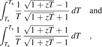
and their analytical solution in the case z(T)T = ko = const.,

Let us further assume that the constant ko is related to the average over z(T)T:
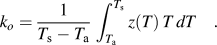
The constraint z(T)T = ko = const. can be considered as an upper/lower bound because the following integral inequalities hold for positive values T s and T a and any given z(T) > 0, such that z(T)T is monotonously increasing:

and

with ko given by Eq. (A3).
Proof: Let g be a continuous, convex (concave) function on ℝ+; then Jensen’s inequality

holds for any nonnegative continuous function y : [a, b] → ℝ (see Ref. Reference Steele15, p. 113). Defining

one easily verifies that g″l(w) < 0 for all w ≥ 0 and g″u(w) > 0 for all w > 0. Hence, g l is concave and gu is a convex function on (0, ∞).
First we prove Eq. (A4). Choosing y(T) = z(T)T we obtain by means of
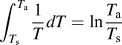
and Eq. (A3) from Jensen’s inequality the following:
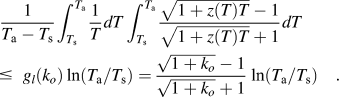
As a second step, we use Chebyshev’s inequality for integrals (see, e.g., Ref. Reference Mitrinovic, Pecaric and Fin16). Let F and G be both monotonically increasing or monotonically decreasing nonnegative functions, respectively, on an interval [a, b]; then, the inequality
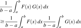
holds. The relation reverses if one of the functions increases and the other decreases. If y(T) = z(T)T is monotonically increasing, then the composition G(T) = (gl ○ y)(T) = gl(z(T)T) increases as well. However, F(T) = 1/T decreases; hence, we obtain from Eq. (A6) the proposed relation (A4).
In the same way we obtain the estimate Eq. (A5) applying Jensen’s inequality on the convex function gu and then Chebyshev’s inequality taking into account that the composition (gu ○ y)(T) = gu(z(T)T) now is a monotonically decreasing function if y = z(T)T increases. ▪
Remark 1: The integral on the left-hand side of Eq. (A5) cannot be bounded above by any constant depending on ko. We give an example from the mathematical point of view. Fix some interval [T a, T s] with T s – T a = 20 (all temperatures in Kelvin), a constant c > 0, and define functions zn(T) > 0 on [T a, T s] by

where n ∈ ℕ. Then zn(T)T is continuous and monotonically increasing for every fixed n and the averages ko are uniformly bounded by c/2 ≤ ko ≤ c for all n ∈ ℕ. However, the corresponding integrals in Eq. (A.5) are unbounded because zn(T)T is chosen to be small for large n. To hold the average k 0 bounded below, this effect is restricted to a subinterval of [T a, T s]. For example, on [T a, T a + 4] we have 0 < zn(T)T ≤ c(1/2)n. Then we estimate
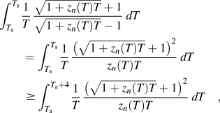
and 0 < zn(T)T ≤ c(1/2)n on [T a, T a + 4] implies that
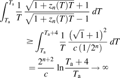
is unbounded as n → ∞.
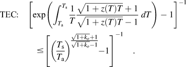
Remark 2: Notice that the proved inequalities Eqs. (A4) and (A5) can be used to estimate the performance parameters. The result is that the quantities (9) serve as upper bounds of the performance values given by the Eqs. (8) if the function z(T)T is monotonically increasing and ko is given by Eq. (A3), because we get the following:
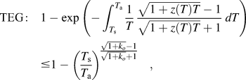
Equality holds if z(T) T = const. If z(T) T is decreasing, however, the above inequalities in general do not hold.