

1. Introduction
The late Dr. John F. Morrall III was an economist who worked in the federal government for over 30 years, first at the Council on Wage and Price Stability and later at the Office of Information and Regulatory Affairs (OIRA) within the US Office of Management and Budget (OMB). One of the authors of this article first met Dr. Morrall at a conference in the late 1970s where Dr. Morrall presented an unpublished table ranking the cost-effectiveness of health and safety regulations at different federal agencies. Morrall’s presentation inspired a graduate student to prepare an even larger table of lifesaving interventions as part of his master’s thesis at Duke University (Graham & Vaupel, Reference Graham and Vaupel1981). Such tables came to be known as lifesaving league tables, borrowing a term that was originally used when ranking British soccer teams from best to worst according to their win-loss records.
We doubt that Dr. Morrall’s lifesaving league table was the very first of its kind. Zeckhauser and Shepard (Reference Zeckhauser and Shepard1976) compared the cost-effectiveness of alternative interventions to treat and prevent coronary heart disease, and Weinstein and Stason (Reference Weinstein and Stason1977) refined cost-effectiveness analysis for medical applications and presented such information in their classes at the Harvard School of Public Health. Schwing (Reference Schwing1979) compared the cost-effectiveness of different large-scale, mortality-reducing programs. And Travis et al. (Reference Travis, Richter, Crouch, Wilson and Klema1987) presented at meetings and eventually published a striking table on the relative cost-effectiveness of different ways to prevent cancer.
Such tabular information may have first been prepared in the Department of Defense to convey the most efficient ways to protect military personnel from noncombat and combat-related hazards (Banzhaf, Reference Banzhaf2014). However, those tables are not publicly available. It is not unreasonable to speculate that this way of thinking was an outgrowth of Robert McNamara’s campaign to bring the tools of systems analysis into the military and civilian sides of the federal government during the Kennedy and Johnson administrations (Tarpgaard, Reference Tarpgaard1995).
Although Dr. Morrall on occasion presented his league table at meetings, there was a long delay before it first appeared in a published public document. Since OMB is a unit within the Executive Office of the President, where communication sensitivities are high, formidable clearance procedures must be surpassed before an analyst can obtain permission to publish in the open literature. We believe Dr. Morrall’s first lifesaving league table appeared in Regulation magazine in 1986 (Morrall, Reference Morrall1986), without attribution to OMB; the next few appeared in official OMB documents in 1988 (OMB, 1988), 1991 (OMB, 1991), 2002 (OMB, 2002) and 2011 (OMB, 2011).
Once Dr. Morrall’s tables were published, they spurred research interest both in the United States and around the world. A Harvard doctoral student dissertation, supported by a grant from the National Science Foundation, compared the cost-effectiveness of 500 lifesaving interventions in the United States (Tengs et al., Reference Tengs, Adams, Pliskin, Safran, Siegel, Weinstein and Graham1995). She also performed a provocative calculation that 60,000 more lives could be saved each year in the United States if resources were reallocated from the less cost-effective interventions to the more cost-effective interventions (Tengs and Graham, Reference Tengs and Graham1996). Soon thereafter, large lifesaving league tables were published using data from interventions in Japan, Sweden and Australia (Kishimoto, Reference Kishimoto1997; Ramsberg and Sjoberg, Reference Ramsberg and Sjöberg1997). More recently, lifesaving league tables have been published in New Zealand and Australia (Dalziel et al., Reference Dalziel, Segal and Mortimer2008; Wilson et al., Reference Wilson, Davies, Brewer, Nghiem, Cobiac and Blakely2019; Carvalho et al., Reference Carvalho, Sousa, Mizdrak, Jones, Wilson and Blakely2022). Although much of the literature focuses on developed countries, scholars have also produced large league tables for low-income and middle-income countries (Horton et al., Reference Horton, Gelband, Jamison, Levin, Nugent and Watkins2017). An especially rigorous league table for medical practices includes only those estimates that meet minimum standards for quality of analysis (Chapman et al., Reference Chapman, Stone, Sandberg, Bell and Neumann2000).
Lifesaving league tables invite readers to infer that entrees at the top of the list (low cost per life saved) are good lifesaving regulations while entrees at the bottom of the list (high cost per life saved) are bad lifesaving regulations. Strictly speaking, the ratios speak only to the relative efficiency of the regulations, without any consideration of equity or fairness or what Congress demanded in the underlying statute.Footnote 1 Dr. Morrall’s tables were especially provocative because they suggested that the Occupational Safety and Health Administration (OSHA) and the Environmental Protection Agency (EPA) were responsible for several regulations with very high cost-effectiveness ratios, leading Judge Richard Posner to lament “astronomical” cost-effectiveness ratios in his favorable opinion about OSHA’s bloodborne pathogens rule (American Dental Association v Martin 984F.2d 823 (7th Cir. 1993)).
Fierce criticisms of Dr. Morrall’s tables were published, especially in the legal literature (e.g. see Heinzerling, Reference Heinzerling1997, Heinzerling, Reference Heinzerling1998; Heinzerling & Ackerman, Reference Heinzerling and Ackerman2001; Parker, Reference Parker2003; Parker, Reference Parker2004; Heinzerling, Reference Heinzerling2005; Parker, Reference Parker2006). The critics made numerous arguments such as the lifesaving league tables ignore statutory requirements faced by agencies, undercount health benefits that are not lifesaving in nature, undercount nonhealth benefits that may be side benefits of lifesaving regulations, ignore ecological benefits, give too much credence to cost estimates based on industry information and apply excessive rates of discount to future lifesaving impacts. In a peer-reviewed journal publication before his retirement, Dr. Morrall made modest adjustments to his methods, expanded his database further and responded to the concerns of some of his critics (Morrall, Reference Morrall2003). Others (Hahn, Reference Hahn2004) also responded to critics.
Critics of lifesaving league tables also raised practical questions about how the tables should be used by decision-makers, since the lifesaving measures in league tables often do not compete for the same resources (Mauskopf et al., Reference Mauskopf, Rutten and Schonfeld2003). Proponents of league tables, like Dr. Morrall, saw them as a device to provide a synoptic perspective on the efficiency of different lifesaving investments and to encourage regulatory reform, not as a tool that would be used mechanically by decision-makers.
In this article, our objective is to build on Morrall’s work by comparing the estimated cost-effectiveness of federal lifesaving regulation in 1967–2001, Period 1, to recent years 2009–2024, Period 2. We excluded rules issued in the G.W. Bush Administration because we worked at OIRA at that time and because the 2009–2024 period proved to be long enough to generate a sizeable sample for comparison. We do not investigate whether the use of benefit–cost analysis supports more or less regulation, and we make no assumption regarding this relationship.
2. Primary hypothesis
Our primary hypothesis is an improvement in the estimated cost-effectiveness of federal lifesaving regulation in Period 2 compared to Period 1. We consider a regulation to be cost-effective if the cost per life saved is less than the value of a statistical life, and an improvement in cost-effectiveness is when the cost per life saved decreases between regulations issued in Period 1 and those issued in Period 2. We expect an improvement in both the average and median cost-effectiveness of regulation. We also expect fewer regulations with extremely large expenditures per life saved. Given a common value-of-statistical life (VSL) measure employed by federal agencies (~$12 million per life saved in 2022) based on the early work of Viscusi and recent agency practices (e.g. see Viscusi, Reference Viscusi1978; Viscusi and Aldy, Reference Viscusi and Aldy2003; Moran, Reference Moran2016; EPA, 2025), we expect a higher percentage of regulations will pass the VSL test (i.e. the cost per life saved is less than the VSL) in Period 2 compared to Period 1.
Our primary hypothesis is based on prior literature, institutional developments in regulatory oversight and our practical experience at OIRA. Period 1 (1967–2001), which was studied by Morrall (Reference Morrall2003), witnessed the boom in social regulation (i.e. rules to improve societal welfare and protect the public from harmful practices), especially health, safety and environmental controls on business. Entirely new agencies were established, such as the National Highway Traffic Safety Administration (NHTSA), the Occupational Safety and Health Administration (OSHA), the Consumer Product Safety Commission (CPSC) and the Environmental Protection Agency. Congress enacted new authorizing legislation, both for the new agencies and the older ones (e.g. the Food and Drug Administration was granted new authority over medical devices in 1976 and food safety in 1992).
By the late 1970s, the average number of new federal rulemakings peaked at more than 7,000 per year, almost double the volume that is typical of recent years. While the overall volume of federal regulation was less in Period 1 than Period 2, the share of regulations with health/safety impacts was substantial in both periods. Based on random sampling, we found that 38% (±5%) of final rules issued in 1995 (n = 4,747) and 46% (±5%) of final rules issued in 2022 (n = 3,168) were intended to improve human health or safety.Footnote 2
Concern about the cost-effectiveness of federal regulation did emerge in Period 1, beginning with a limited degree of White House oversight of federal regulators in the 1970s through the activities of the Council on Wage and Stability, the Council of Economic Advisors and OMB (Hopkins, Reference Hopkins2011). In 1981, President Ronald Reagan established OIRA based on statutory authorization in the Paperwork Reduction Act of 1980 and imposed the first benefit–cost test on new regulations. However, the agencies and their allies in Congress resisted the new analytical requirements; a backlash in Congress almost led to the abolition of OMB oversight of regulators. OIRA survived but only after a 50% reduction in staffing, new disclosure requirements and a requirement that the OIRA administrator be confirmed by the Senate. Under the 4-year administration of George Herbert Walker Bush, the Senate refused to confirm an OIRA nominee (Graham, Reference Graham2024). It was not until the 8-year Clinton administration (1993–2001) that OIRA oversight of federal regulators became more widely accepted by leaders of both political parties. The value of OIRA, or any central oversight of regulatory matters, includes ensuring consistency in the conduct of benefit–cost analysis and the cost-effectiveness of regulation (Broder and Morrall, Reference Broder and Morrall1997). Yet even with such centralized oversight, the quality of analysis may differ across presidential administrations (Ellig et al., Reference Ellig, McLaughlin and Morrall2013).
In recent decades, the judicial branch has emerged as a check on the power of regulators to issue regulations with extremely high costs per life saved and as a check on the power of deregulators to eliminate regulations with a relatively small cost per life saved. Professor Cass Sunstein of Harvard Law School referred to this development as the “cost–benefit” state (Sunstein, Reference Sunstein2002). Although there are a few regulatory statutes that prohibit consideration of cost (e.g. the National Primary Ambient Air Quality Standards under the Clean Air Act), the courts have found that the wording of most statutes is flexible enough to allow (or even require) consideration of the cost of lifesaving regulations. Even if an agency’s authorizing statute does not explicitly authorize consideration of costs, courts have found that the “arbitrary and capricious” standard of judicial review under the Administrative Procedure Act of 1946, which covers all federal departments and agencies, contains an implicit requirement that regulators balance costs and benefits (Noe and Graham, Reference Noe and Graham2019). Thus, compared to the 1970s, regulators today realize that a rulemaking that imposes “astronomical” costs per life saved is vulnerable to judicial reversal.
Finally, federal agencies themselves have become more open to economic reasoning and evidence. In the 1970s, those new federal agencies created to address social regulation employed few PhD level economists. Back then, the pipeline of civil servants seldom included training in economic analysis. Most law schools did not yet have a “law and economics” curriculum, and most master’s degree programs in public administration and public affairs did not require training in the tools of benefit–cost analysis. Much has changed since then. EPA was one of the first agencies to establish a branch of economists and give them some role in reviewing the rulemaking proposals of EPA’s program offices (Graham, Reference Graham2024). Other social agencies followed suit to various degrees. And most law schools now have at least some law and economics curricula while most public administration and policy programs now teach benefit–cost analysis, often in the core curriculum. Thus, while there remain pockets of resistance to economic analysis and OIRA oversight of regulators, it is much more accepted today than in Period 1 that lifesaving regulations (and deregulatory actions) should be scrutinized for their cost-effectiveness.
In making our primary hypothesis, we assume that the underlying problems to be addressed by regulation in Period 2 are as easy to address as the underlying problems addressed in Period 1. But the possibility of a difference cannot be ruled out. For example, regulators may choose to pick the lowest hanging fruit first, suggesting greater cost effectiveness for the first rules issued by a regulatory program compared to later rules. If we find that cost-effectiveness does not differ between the two periods, we cannot rule out the possibility that regulatory impact analysis did improve cost-effectiveness but for the reduction in the ease of control of the underlying problem. Conversely, if we find that Period 2 rules are not as cost-effective as those in Period 1, we cannot conclude that the application of benefit–cost analysis made matters worse.
3. Data and methods
To facilitate temporal comparison, we employed the same effectiveness metric that Morrall employed even though his method is slightly different than the method currently used in public health and medicine. Specifically, although health effectiveness is now typically measured as the number of quality-adjusted life years (QALYs) saved, we use the number of “equivalent lives saved” (ELS). An advantage of QALYs is that they account for duration as well as the quality of life saved. During the period covered by Morrall’s study, QALYs were not yet in widespread use, especially at federal agencies. ELS is a metric pioneered by analysts at NHTSA; it combines information on the number of lives saved and the number of nonfatal injuries averted, using weights to translate the nonfatal injuries into fatality equivalents (i.e. more severe injuries receive larger weights than less severe injuries). As described below, we adapted the ELS metric so that it could be used for rules that prevent nonfatal illnesses as well as injuries.
Our task collecting data was easier than the task faced by Dr. Morrall. We leveraged OMB’s Annual Report to Congress on the Costs and Benefits of Federal Regulation. Required by statute in 2000, this report includes a table identifying those major regulations reviewed by OMB in draft form before issuance and for which the issuing agency quantified at least some of both costs and benefits. For those rulemakings, we then obtained the regulatory impact analysis (RIAs) prepared by the issuing agency to determine if it contained sufficient information to determine the expected annual cost and expected annual number of lives saved and that it met the Morrall criteria for inclusion (only final rules that were not rejected through legislative or judicial action, the life-saving benefits represent the majority of monetized benefits, and monetized nonhealth benefits do not exceed compliance costs). If so, we deemed the rule in-scope and included the rule in our list. For rules issued since FY2023 (the last time OMB issued its annual report), we searched the Semiannual Agenda of Regulatory and De-Regulatory Actions and the Federal Register to identify those rules that met the Morrall inclusion criteria. We also searched for and added regulations that were not designated as major rules and otherwise met the Morrall criteria for inclusion.
For each in-scope regulation, we coded the issuing agency, date of publication in the Federal Register, stage of rulemaking, regulatory identification number, whether the rule was required or discretionary, the initial risk of mortality per 10,000 exposed people, the initial number of deaths in the exposed US population, the average annual number of lives saved and ELS expected under the rule and the average annual cost of the rule using a discount rate of 7% (to reflect the opportunity cost of capital, to maintain consistency with Morrall (Reference Morrall2003)). We divided annual cost by ELS to obtain the opportunity cost per statistical life saved (OCSLS) – the same cost effectiveness measure used by Morrall in his 2003 league table. In the few cases where ELS was not estimated nor could be discerned, we used lives saved instead.
For each in-scope regulation, we adjusted agency-derived estimates of annual cost to reflect constant 2022 dollars. If the issuing agency did not provide the expected number of annual lives saved and/or equivalent lives saved but did monetize human health benefits, we estimated it from the available information. In no instance did we conduct original analysis to substitute for the agency’s analysis. Our intent was to ensure that estimates of costs and benefits reflect the agency analysis, and we used this information to develop a cost-effectiveness ratio for each rule.
Morrall’s Reference Morrall2003 table, which is likely a complete list of monetized life-saving rules over 34 years, included 76 rules. We found 67 in-scope rules over a 16-year period. We also found 51 additional rules for which both costs and health benefits were monetized but which failed to meet one or more of the Morrall criteria for inclusion. In most of these cases, monetized energy savings exceeded monetized health benefits, such as for 35 DOE energy conservation standards, as well as several major regulations involving control of greenhouse gas emissions from the power sector, motor vehicle fuel economy standards and CO2 tailpipe standards for motor vehicles.
To test our primary hypothesis, we compared the resulting cost-effectiveness ratios for the in-scope regulations in Periods 1 and 2. We computed the percentage of rules with ratios less than or greater than the VSL and 10× VSL for each period, reasoning that the VSL represents the boundary of cost-effectiveness, and 10× VSL represents egregiously poor cost-effectiveness. It reflects the mortality cost of expenditures (MCE) (Broughel and Viscusi, Reference Broughel and Viscusi2021), above which a regulation may add to, rather than prevent, premature mortality because it diverts resources that might otherwise be directed to health-enhancing expenditures.Footnote 3
4. Primary results
Table 1 presents the lifesaving league table for Period 2 (2009–2024), indicating the name of the regulation, the year the final rule was published in the Federal Register, the issuing agency and the cost-effectiveness measured as the OCSLS. The regulations are listed in descending order of cost-effectiveness, with the most cost-effective rules at the top.
Cost-effectiveness of selected federal life-saving regulations, 2009–2024

Table 1. Long description
The table contains four columns: Regulation, Year, Agency, and Opportunity cost per statistical life saved (millions of 2022 dollars). The data is sorted by cost from lowest to highest.
* Interstate transport of P M and ozone (2011, E P A): 0.04
* Residential wood heaters (2015, E P A): 0.1
* Adult portable bed rails (2023, C P S C): 0.1
* M C L P F A S (2024, E P A): 0.2
* N E S H A P: integrated iron and steel (2024, E P A): 0.2
* Boiler M A C T reconsideration (2013, E P A): 0.3
* P M N A A Q S (2013, E P A): 0.3
* Cross-state air pollution – 2008 ozone N A A Q S (2016, E P A): 0.3
* Salmonella in shell eggs (2009, F D A): 0.4
* Sulfur dioxide N A A Q S (2010, E P A): 0.4
* Child-restraint systems: side impact protection (2022, N H T S A): 0.5
* Repeal of the clean power plan and A C E (2019, E P A): 0.6
* Seatbelts on motor coaches (2013, N H T S A): 0.6
* Portland cement N E S H A P and N S P S (2010, E P A): 0.9
* Anti-ejection glazing for motor coaches (2024, N H T S A): 0.9
* Cranes and derricks (2010, O S H A): 0.9
* Effluent limitation guidelines for E G Us (2024, E P A): 1.0
* Occupational exposure to beryllium (2017, O S H A): 1.0
* N E S H A P: acid gas standards (2020, E P A): 1.3
* Organ procurement H O P E Act (2024, H H S): 1.4
* Ejection mitigation (2011, N H T S A): 1.5
* Food labeling rule delay (2018, F D A): 1.5
* Coal- and oil-fired E G U N E S H A P (2012, E P A): 1.6
* Nutritional labeling on menus (2014, F D A): 1.8
* Brick and clay N E S H A P (2015, E P A): 2.2
* Heavy-duty engine and vehicle standards (2023, E P A): 2.2
* Sound for hybrid and electric vehicles (2016, N H T S A): 2.3
* Head start vaccine and mask mandate (2021, H H S): 2.4
* N E S H A P: R I C E (2010, E P A): 2.5
* Bus rollover structural integrity (2021, N H T S A): 2.8
* Blood transfusion testing (2015, F D A): 2.9
* R I C E reconsideration (2013, E P A): 3.1
* Mammography standards (2023, F D A): 3.2
* Electrical protective equipment (2014, O S H A): 3.2
* Ozone N A A Q S (2015, E P A): 3.5
* H O N (2024, E P A): 3.7
* Hours of service (2011, F R A): 3.8
* Standards for produce (2015, F D A): 3.9
* G M P, infant formula (2014, F D A): 4.1
* Revoke the use of partially hydrogenated oils in foods (2023, F D A): 5.2
* Rear impact guards for trucks (2022, N H T S A): 5.2
* Confined spaces (2015, O S H A): 7.3
* Roof crush resistance (2009, N H T S A): 7.9
* Industrial, commercial, and institutional boilers and process heaters (2022, E P A): 8.6
* Commercial driver’s license drug and alcohol clearinghouse (2016, D O T): 8.9
* Fall protection systems (2016, O S H A): 9.8
* Perchloroethylene (2024, E P A): 10.6
* Organ procurement organizations, conditions for coverage (2020, H H S): 14
* Lowering miners’ exposure to coal mine dust (2014, D O L): 16.3
* N E S H A P: coal- and oil-fired E G Us (2024, E P A): 24.9
* F M V S S: rear visibility (2014, N H T S A): 26.3
* Activation of ice protection (2011, F A A): 33.78
* Phasedown of H F Cs: restrictions on the use of certain H F Cs (2023, E P A): 36
* Airport safety management system plan (2023, F A A): 38.3
* Operating cords for custom window coverings (2022, C P S C): 41.9
* Formaldehyde in composite wood products (2016, E P A): 52
* Trichloroethylene (2024, E P A): 54
* Methylene chloride (2024, E P A): 55.9
* Pilot certification for air carriers (2013, F A A): 113.6
* Positive train control (2010, F R A): 179.9
* Positive train control amendments (2012, F R A): 299.1
* Carbon tetrachloride (2024, E P A): 791
* N E S H A P: M O N (2020, E P A): 3,578
* Oil and natural gas sector: emission standards (2020, E P A): 5,208
* Phasedown of H F Cs: allowance allocation methodology for 2024 and later years (2023, E P A): 17,676
* Asbestos, Part 1 (2024, E P A): 93,760
a This is a deregulatory action.
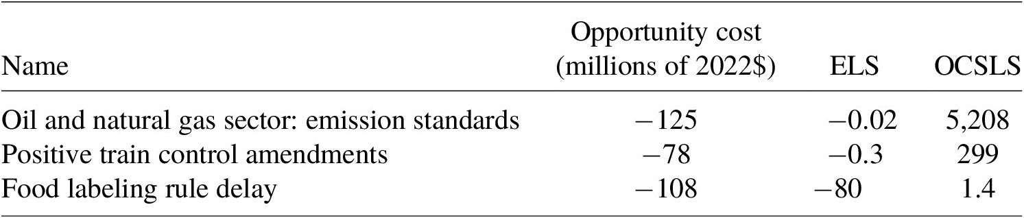
Deregulatory actions, in which an agency reduces both the cost and benefits of an existing regulation, can also be ranked in terms of cost effectiveness, but require special treatment when placed in a league table. Table 2 lists the three deregulatory actions from Table 1. Once again, we list the most cost-effective regulation at the top, but for deregulation, cost-effectiveness is associated with a higher OCSLS value. This is because the cost savings (a negative value) are much larger than the slight reduction in health benefits (also a negative number), resulting in a high, positive number. For this reason, we recommend that deregulatory rules be presented in their own league table where OCSLS is listed from highest to lowest – the opposite of that for regulatory actions.
Deregulatory rules

Table 2. Long description
The table consists of four columns: Name, Opportunity cost (millions of 2022 dollars), E L S, and O C S L S.
* Row 1: Oil and natural gas sector: emission standards. Opportunity cost is minus 125. E L S is minus 0.02. O C S L S is 5,208.
* Row 2: Positive train control amendments. Opportunity cost is minus 78. E L S is minus 0.3. O C S L S is 299.
* Row 3: Food labeling rule delay. Opportunity cost is minus 108. E L S is minus 80. O C S L S is 1.4.
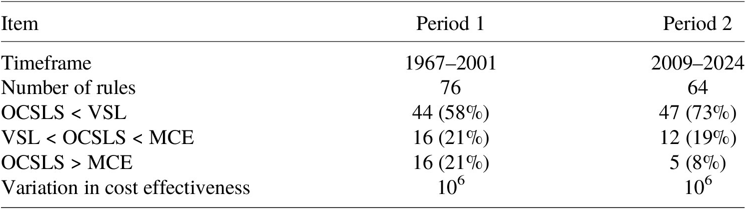
Comparing regulatory league tables for Periods 1 and 2 (Table 3), we find that cost-effectiveness has improved. Both the mean and median OCSLS are lower for regulations in Period 2 than in Period 1. For Period 1, the mean OCSLS is $4,183 million and the median OCSLS is $6.3 million. For Period 2, the mean and median OCSLS are $2,476 million and $3.7 million, respectively. These values are expressed in constant 2022 dollars to ensure a valid comparison across periods.
Comparison of league tables, Period 1 and Period 2

Table 3. Long description
The table consists of three columns: Item, Period 1, and Period 2.
* Timeframe: Period 1 covers 1967 to 2001. Period 2 covers 2009 to 2024.
* Number of rules: Period 1 has 76 rules. Period 2 has 64 rules.
* O C S L S less than V S L: Period 1 shows 44 (58 percent). Period 2 shows 47 (73 percent).
* V S L less than O C S L S less than M C E: Period 1 shows 16 (21 percent). Period 2 shows 12 (19 percent).
* O C S L S greater than M C E: Period 1 shows 16 (21 percent). Period 2 shows 5 (8 percent).
* Variation in cost effectiveness: Both Period 1 and Period 2 show a value of 10 super 6.
Table 3 shows the percentage of regulations that are relatively cost-effective (below the VSL), not cost-effective (greater than the VSL but less than the MCE) and decidedly not cost-effective (greater than the MCE). In Period 1, 58% of the rules were cost-effective, 21% not cost-effective and 21% decidedly not cost-effective. In Period 2, 73% of life-saving rules were cost-effective, 19% not cost-effective and 8% decidedly not cost-effective. The life-saving rules in Period 1 spanned six orders of magnitude in cost-effectiveness, and in Period 2 the span was also six orders of magnitude.
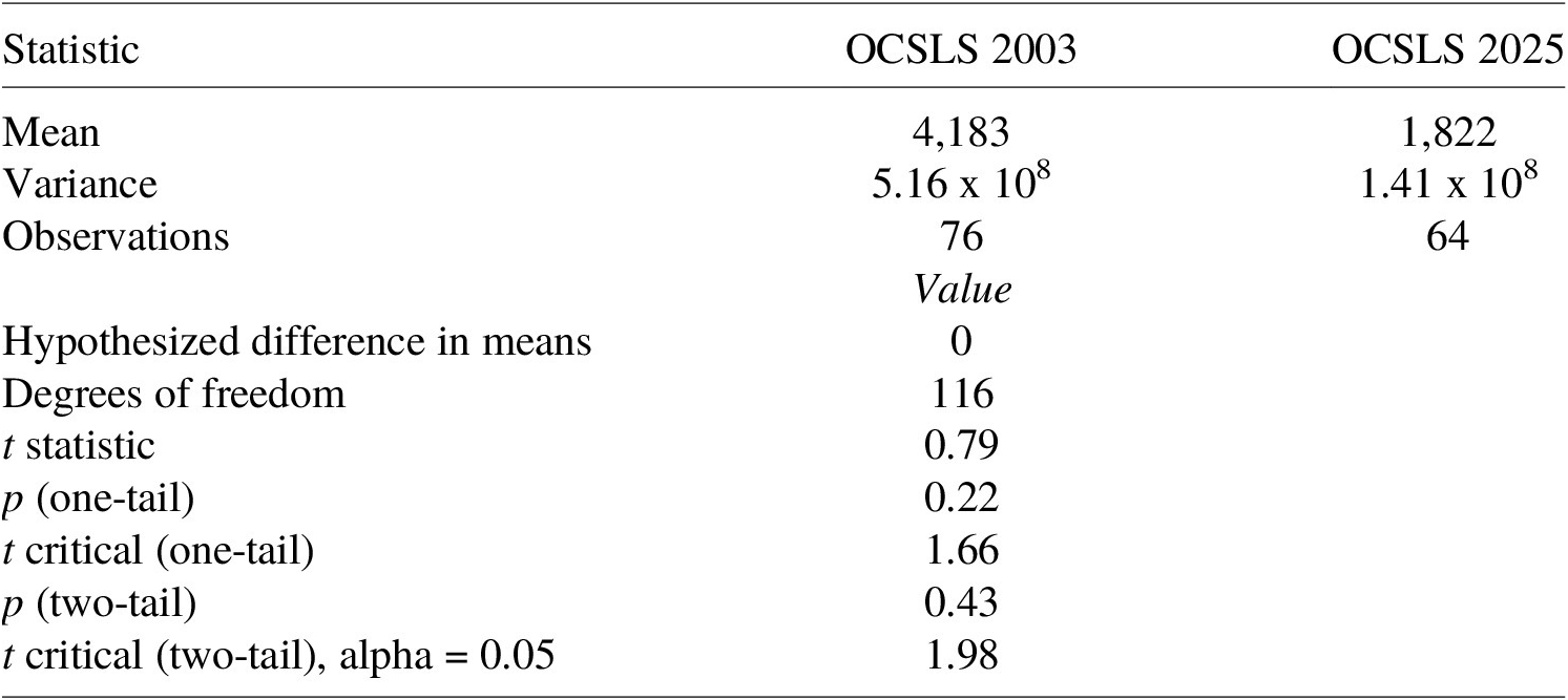
To determine if the observed difference in cost effectiveness is statistically significant, we conducted an F test (which indicated unequal variance) followed by a two-tailed t test, the results of which (Table 4) do not allow us to reject the null hypothesis of equal means in cost-effectiveness because the t statistic is less than the t critical value using a two-tailed test.
Statistical comparison of mean cost-effectiveness in OCSLS data sets

Table 4. Long description
The table consists of three columns: Statistic, O C S L S 2003, and O C S L S 2025.
Comparative data for the two years:
* Mean: 4,183 for 2003 and 1,822 for 2025.
* Variance: 5.16 times 10 super 8 for 2003 and 1.41 times 10 super 8 for 2025.
* Observations: 76 for 2003 and 64 for 2025.
Statistical test values (Value column):
* Hypothesized difference in means: 0.
* Degrees of freedom: 116.
* t statistic: 0.79.
* p (one-tail): 0.22.
* t critical (one-tail): 1.66.
* p (two-tail): 0.43.
* t critical (two-tail), alpha equals 0.05: 1.98.
5. Additional results
Beyond our primary finding of improved (but not statistically significant) cost-effectiveness, we garnered some additional insights from the league tables. These results do not flow from ex ante hypotheses; they are patterns that we observed when analyzing the data.
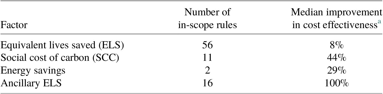
As we compiled the league table for Period 2, we were struck by the extent to which cost-effectiveness was enhanced by certain factors. Table 5 lists these factors, their frequency and the improvement in OCSLS. Using equivalent lives saved over lives saved increased cost-effectiveness somewhat, but only in rare cases (e.g. FDA standards for produce) did monetized morbidity gains overwhelm monetized mortality gains in terms of overall health effectiveness. Using the social cost of carbon (SCC) made a more substantial difference.Footnote 4 However, the largest difference was made by including ancillary lives saved (also known as co-benefits) that do not represent the target risk intended to be reduced. The most common ancillary benefits were those associated with reductions in emissions of small particulate matter when regulating hazardous air pollutants from industrial sources (e.g. acid gas standards for electric generating units, brick and clay NESHAP, RICE and HON). Savings in energy expenditures – which we subtract from annual cost in the numerator of the cost-effectiveness ratio in accordance with the Morrall criteria – also enhance cost-effectiveness (e.g. asbestos Part 1).Footnote 5 We note that many of the rules we excluded based on the Morrall criteria are due to energy savings exceeding compliance cost.
Factors that improve cost effectiveness, Period 2

Table 5. Long description
The table consists of three columns: Factor, Number of in-scope rules, and Median improvement in cost effectiveness (measured as the percentage change in O C S L S after the factor is included).
* Equivalent lives saved (E L S): 56 in-scope rules with an 8 percent median improvement.
* Social cost of carbon (S C C): 11 in-scope rules with a 44 percent median improvement.
* Energy savings: 2 in-scope rules with a 29 percent median improvement.
* Ancillary E L S: 16 in-scope rules with a 100 percent median improvement.
a Measured as the percentage change in OCSLS after the factor is included.
Morrall (Reference Morrall2003) observed that safety regulations (from DOT, DOL and CPSC) tended to be more cost-effective than health regulations (from HHS and EPA). For Period 2 rules, we make a similar observation. Table 6 shows how the 64 regulations (we exclude the three deregulatory rules) compare in terms of cost-effectiveness. Notably, only one safety regulation exceeds the MCE, whereas 9% of the health regulations do. About 70% of both safety and health regulations are cost-effective in that OCSLS < VSL.
Comparison of health versus safety regulation, Period 2 rules

Table 6. Long description
The table is organized into four columns. The first column lists the Category. The next three columns are grouped under the heading Number of regulations by cost effectiveness, divided by the following criteria: O C S L S less than V S L, V S L less than O C S L S less than M C E, and O C S L S greater than M C E.
* Safety regulation row: 15 regulations (71 percent) meet the first criterion, 5 regulations (24 percent) meet the second, and 1 regulation (5 percent) meets the third.
* Health regulation row: 32 regulations (74 percent) meet the first criterion, 7 regulations (16 percent) meet the second, and 4 regulations (9 percent) meet the third.
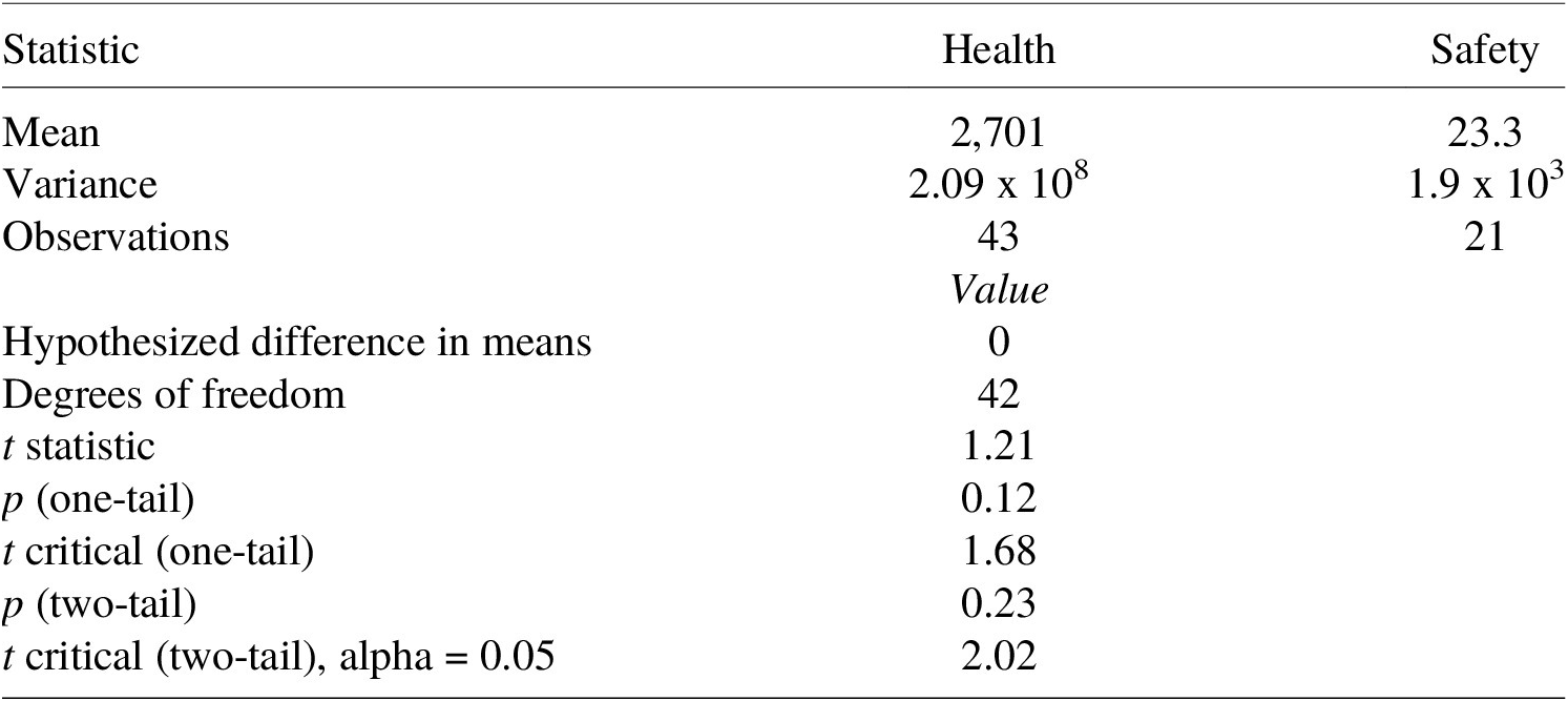
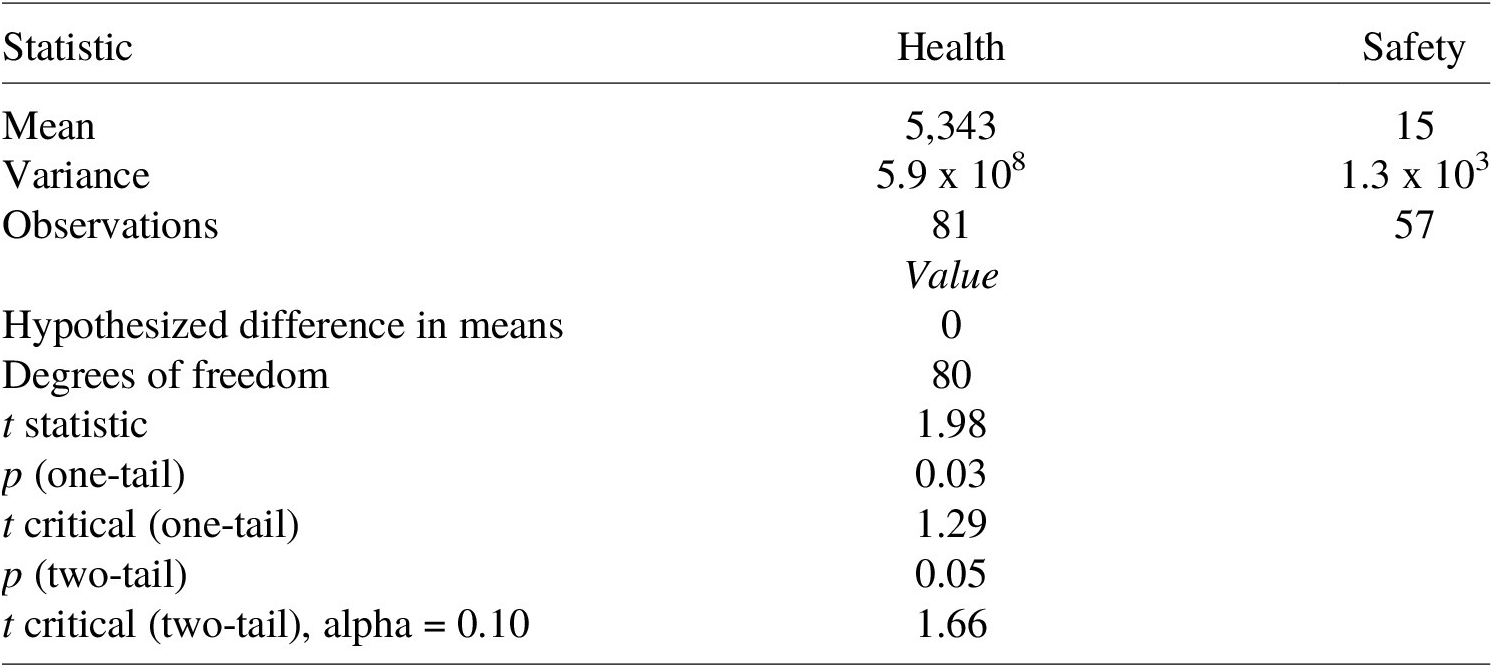
To determine if this difference in safety and health rules is statistically significant, we conducted an F test (which indicated unequal variance) followed by a t test, the results of which (Table 7) do not allow us to reject the null hypothesis of equal means in cost-effectiveness – the t statistic is less than the t critical value using a two-tailed test. We performed a similar analysis for Period 1 rules, the results of which were also not significant at the 95 and 90% confidence levels. To increase the sample size and the degrees of freedom, we combined the health and safety rules in Period 1 and Period 2 (Table 8). At the 90% confidence level (but not at the 95% confidence level), we can reject the null hypothesis. Safety regulations are more cost-effective than health regulations.
Statistical comparison of health versus safety regulation, Period 2 rules

Table 7. Long description
The table is organized into three columns: Statistic, Health, and Safety.
Summary Statistics:
* Mean: Health is 2,701; Safety is 23.3.
* Variance: Health is 2.09 times 10 super 8; Safety is 1.9 times 10 super 3.
* Observations: Health has 43; Safety has 21.
Hypothesis Testing (Value column):
* Hypothesized difference in means: 0.
* Degrees of freedom: 42.
* t statistic: 1.21.
* p (one-tail): 0.12.
* t critical (one-tail): 1.68.
* p (two-tail): 0.23.
* t critical (two-tail), alpha equals 0.05: 2.02.
Statistical comparison of health and safety regulations, combined data

Table 8. Long description
The table consists of three columns: Statistic, Health, and Safety.
* Mean: Health is 5,343; Safety is 15.
* Variance: Health is 5.9 times 10 super 8; Safety is 1.3 times 10 super 3.
* Observations: Health is 81; Safety is 57.
The following comparative values are listed under the Health column or centered across the row:
* Hypothesized difference in means: 0.
* Degrees of freedom: 80.
* t statistic: 1.98.
* p (one-tail): 0.03.
* t critical (one-tail): 1.29.
* p (two-tail): 0.05.
* t critical (two-tail), alpha equals 0.10: 1.66.
In his first published league table (Morrall, Reference Morrall1986), Morrall reported the risk of premature mortality in the exposed population to be addressed by the regulation. In compiling a league table for Period 2, we included, for each rule, an estimate of mortality risk, the baseline number of fatalities in the exposed population and the expected number of lives saved by the rule. We reasoned that the larger the expected risk reduction (expected number of lives saved divided by the baseline fatalities in the exposed population), the more cost-effective the regulation. In other words, the bigger the target, the easier it would be to land a bullseye. Furthermore, we reasoned that the relationship would be stronger for discretionary rules (those without a statutory or court-ordered deadline or those not prescribed explicitly by the underlying statute) where regulators have fewer constraints and stronger still for discretionary rules absent consideration of ancillary ELS (because the ancillary benefits mask the cost-effectiveness of the target risk). However, a visual examination of the scatterplots indicated no apparent relationship. For each of the three data sets (all rules, discretionary rules and discretionary rules absent ancillary benefits), an ordinary least squares analysis reveals a p-value well above the 5% threshold. Goodness-of-fit tests (R-squared) were also very low.
Our results are suggestive of an improvement in cost-effectiveness of regulations issued in Period 2 compared to those issued in Period 1. However, because regulations were not chosen at random, we cannot rule out confounding factors that might influence the results, such as a difference in the ease of control. To the extent that regulators address the lowest hanging fruit first, our results become more suggestive of a positive relationship between the application of benefit–cost analysis and the cost-effectiveness of federal regulation.
6. Discussion
The use of league tables by OMB was guided by the belief that benefit–cost analysis could lead to more efficient and effective regulation. This “smart regulation” concept was expressed by Dr. Morrall in his 30 September 2013 testimony before the House Committee on the Judiciary Subcommittee on Regulatory Reform, Commercial and Antitrust Law (U.S. Congress, 2013):
while at OIRA, I developed league tables of risk regulations and found that the cost-effectiveness of final regulations aimed at saving lives can vary by several orders of magnitude. The findings imply that a better system of setting priorities when it comes to regulation could save [an additional] thousands of lives while saving billions of dollars by focusing time and effort on issuing regulations that could save more lives at lower costs.
This efficiency argument is often made by those who develop league tables of regulation. It is also apparent from our collection of Period 2 rules. If regulators were to rescind just those “egregious” regulations where OCSLS > MCE, $1.2 billion and 104 statistical lives could be saved every year. Alternatively, if regulatory costs were held constant but the costs associated with egregious rules reallocated toward “non-egregious” rules with median cost-effectiveness, an additional 550 statistical lives could be saved every year.
If the efficiency gains are so apparent, why are cost-ineffective regulations issued? Shapiro (Reference Shapiro2005) argued that political factors explain why OIRA is limited in its ability to facilitate more protection at less cost. Building on this idea, Shapiro and Morrall (Reference Shapiro and Morrall2012) examined a small sample of regulations and found that economic analysis is most impactful when political salience is low.
Our compilation of lifesaving regulations in Period 2 illustrates four practical limitations of smart regulation. Statutory discretion matters. The degrees of freedom afforded to regulatory agencies by statute are wide-ranging. In some cases, regulatory programs intended to save lives are so prescribed in detail by statute that cost effectiveness is difficult to achieve in practice. This is true for EPA’s regulatory program to reduce hazardous air pollutants (HAPS) from industrial sources. Under this Clean Air Act program, the agency must control pollutants based on the maximum achievable control technology, irrespective of risk and cost. After a period of years, the agency is required to revisit these controls (known as a risk and technology review), when a minimum risk level must be maintained, and technology controls may be added to ensure the maximum technology continues to drive emission reductions. Under this program, cost-effectiveness tends to be poor – an outcome that Congress was aware of at the time of enactment (Goldstein, Reference Goldstein1989). None of the Period 2 regulations issued under this program are cost-effective due to reductions in hazardous air pollutants; ancillary lives saved (from reductions in particulate matter that occur simultaneously with reductions in HAPS) drive cost-effectiveness.
Effective interagency coordination remains difficult to achieve. In practice, regulatory agencies are focused on their mission that is created by statute at Congress’ direction, and agency missions tend to be narrowly focused. This impediment to smart regulation has long been recognized. DeMuth recommended the establishment of a regulatory budget akin to the well-established fiscal budget, in which regulatory agencies are constrained in issuing rules that are not aligned within a budget determined by the president and Congress (DeMuth, Reference DeMuth1980). We note that the Trump Administration has announced its intention to constrain agency rulemakings by requiring deregulatory cost savings equal to or greater than the costs of new regulations. In theory, an agency wishing to impose regulatory costs in excess of its deregulatory cost savings can do so through interagency trading conditioned on the approval of OMB. Although we are not aware of such interagency trading, such a development would represent a step-change toward smart regulation.
Public and congressional opinion, influenced by media stories and advocacy groups, sometimes contributes to cost-ineffective regulation. Sometimes regulators issue a regulation that is egregious in terms of cost-effectiveness (greater than the MCE) because the underlying hazard is deemed unacceptable (e.g. asbestos, Part 1). In other cases, cost-effective risk-reducing regulations remain on the shelf because the risk management approach is deemed unacceptable (e.g. FDA’s 2022 proposed ban of menthol cigarettes, which was never finalized; OSHA’s 2021 vaccine mandate to address COVID was vacated by the Supreme Court in early 2022). In both examples, cost-effectiveness was not compelling enough to overcome other criteria of importance.
Identifying reasonable regulatory alternatives often falls short of best practice. While compiling our modern league table, we found several instances where an agency RIA fell short of established guidelines (e.g. not offering at least one more stringent and one less stringent alternative). We found that agencies seldom identify regulatory alternatives that challenge an agency’s preferred regulatory option. This is contrary to the intent of an RIA, which is to discover a regulatory alternative that maximizes net benefits while adhering to the Agency’s statutory authority.Footnote 6
Together, these four observations limit the promise of more protection at less cost through the use of benefit–cost analysis. We note, however, that the identification of regulatory alternatives in an RIA is often completely under the control of the regulatory agency – it neither requires an action by Congress nor the President – and can be improved relatively easily and quickly. It can originate within an agency or across agencies with OMB oversight.
Our results also suggest three promising research directions. The cost-effectiveness information in this article is drawn entirely from ex ante regulatory impact analyses by agencies seeking to support a final rulemaking. It is well known, based on selective retrospective studies, that ex post estimates of cost and lifesaving do not necessarily validate the estimates made ex ante (Harrington et al., Reference Harrington, Morgenstern and Nelson2000). Yet we found no lifesaving league tables based entirely on ex post information. As the body of ex post information from retrospective studies improves, we recommend that lifesaving league tables be compiled with ex post information. Second, we recommend that the noted difference in cost-effectiveness between safety and health regulation be investigated further to determine the relative importance of various underlying factors (e.g. statutory direction on benefit–cost considerations). Third, we note that energy-saving regulations represent a class of major regulations suitable for a league table using a methodology like that used for life-saving regulations (i.e. only regulations where the majority of the monetized benefits are energy saving versus lifesaving).
Although benefit–cost analysis was historically seen as a technocratic tool to inform regulators and emphasize economic efficiency, it is no longer ignored by elected officials. The Reagan Administration greatly expanded its use in the form of regulatory impact analysis, which was seen as a tool to restrain overzealous regulators. Since then, it has been employed to justify ever-more stringent major regulations. Recent policy choices are changing how benefit–cost analysis is employed – especially for environmental rules. The Biden Administration revised OMB guidelines on benefit–cost analysis in ways that allowed agencies more discretion while at the same time issuing a record number of major regulations in terms of both costs and benefits (Belton, Reference Belton2022). The Trump administration, with its focus on deregulation, reverted to the old OMB guidelines and is reconsidering many of the Biden regulations. It halted monetization of climate benefits using the social cost of carbon (a figure which EPA had raised in the Biden Administration) in federal regulatory and permitting decisions, which led to repeal of major regulations on automobiles and power plants. It halted the monetization of benefits associated with reductions in PM2.5 and ozone in air pollution regulations, a move predicated on uncertainty in the underlying science, which had long been acknowledged. In a turn away from Reaganism (Fraas et al., Reference Fraas, Lutter and Viscusi2026), deregulation now relies less on benefit–cost analysis while emphasizing the single best reading of a statute, per the Supreme Court’s 2024 opinion in Loper Bight Enterprises v. Raimondo. These recent policy changes reduce both the costs and benefits of regulation and decrease monetized cost-effectiveness. In the long run, Congress is likely to be more prescriptive – but not necessarily more stringent – when authorizing new regulatory activity. The impact on cost-effectiveness is unclear.
Acknowledgments
The authors would like to thank current and former OIRA staff for helping them gather relevant information and providing helpful feedback. David Lan and Jax Fischer supplied useful research assistance.



 Open access

