



1 Introduction
Diseased or defective human heart valves are routinely replaced with prosthetic valves, with approximately 280 000 valve replacements implanted worldwide, each year (Pibarot & Dumesnil Reference Pibarot and Dumesnil2009). The most common valve surgical procedure is aortic valve replacement for aortic stenosis (Roberts & Ko Reference Roberts, Ko, Wang and Bashore2009). Of all prosthetic valves, approximately half are mechanical (man-made) and half are bioprosthetic (from an animal or human) (Pibarot & Dumesnil Reference Pibarot and Dumesnil2009). Compared with bioprosthetic valves, mechanical valves are more durable and insusceptible to calcification and tearing. Bileaflet mechanical heart valves (BMHVs) are the most widely implanted valve today (Dasi et al. Reference Dasi, Simon, Sucosky and Yoganathan2009) and account for 80 % of implanted mechanical valves (Yoganathan et al. Reference Yoganathan, Leo, Travis, Teoh, Milne, Ritchie and Karihaloo2003).
Despite their advantages, BMHVs exhibit a high incidence of thrombosis, and recipients are required to take life-long anti-coagulation therapy to prevent thromboembolic complications (Sotiropoulos, Le & Gilmanov Reference Sotiropoulos, Le and Gilmanov2016). It is believed that this problem is the result of non-physiological flow patterns generated by the valve, which impose high levels of viscous shear stress and turbulence on the blood elements, eventually damaging them and leading to the formation of thrombi (Dasi et al. Reference Dasi, Simon, Sucosky and Yoganathan2009; Sheriff et al. Reference Sheriff, Bluestein, Girdhar and Jesty2010). In particular, it has been found that high levels of viscous and turbulent stresses occur in the shear layers at the edges of the three jets that issue from the valve’s orifices (Yoganathan, Woo & Sung Reference Yoganathan, Woo and Sung1986; Liu, Lu & Chu Reference Liu, Lu and Chu2000) and high levels of viscous stress occur in the flow through the leaflet hinges (Sotiropoulos et al. Reference Sotiropoulos, Le and Gilmanov2016).
The ascending aorta is highly non-axisymmetric, having three lobed sinuses at its root, which accommodate the three leaflets of the native aortic valve. Two of these sinuses branch into coronary arteries, which supply the heart muscle with oxygenated blood. The flow in these arteries is dependent on the recirculating flow in the sinuses (Carroll & Falsetti Reference Carroll and Falsetti1976; De Paulis et al. Reference De Paulis, Tomai, Bertoldo, Ghini, Scaffa, Nardi and Chiariello2004), which has been characterized as a three-dimensional vortex ring by Dasi et al. (Reference Dasi, Ge, Simon, Sotiropoulos and Yoganathan2007) and Borazjani, Ge & Sotiropoulos (Reference Borazjani, Ge and Sotiropoulos2010). Downstream of the root, the ascending aorta and the aortic arch are also highly non-axisymmetric, curving in two planes (Chandran Reference Chandran1993). Unlike the native aortic valve and its counterpart, the aortic sinus, which are approximately triradially symmetric, the BMHV is bilaterally symmetric (figure 1). This mismatch of symmetry between the BMHV and the surrounding channel raises the question of how the valve’s orientation relative to the aorta affects the flow downstream of it. Animal studies have confirmed that BMHV orientation affects the flow patterns (Mächler et al. Reference Mächler, Perthel, Reiter, Reiter, Zink, Bergmann, Waltensdorfer and Laas2004), turbulence (Kleine et al. Reference Kleine, Perthel, Nygaard, Hansen, Paulsen, Riis and Laas1998) and coronary flow (Kleine et al. Reference Kleine, Scherer, Abdel-Rahman, Klesius, Ackermann and Moritz2002) past the valve, and have guided clinical practice. The clinical experience of Aoyagi et al. (Reference Aoyagi, Tanaka, Nishi, Yamashita, Oryouji, Hara, Kosuga and Ooishi1991) at the Kurume Medical School has indicated that BMHV orientation is one factor that affects hemolysis (Akutsu, Imai & Deguchi Reference Akutsu, Imai and Deguchi2005). The implantation and orientation of a BMHV is highly dependent on the skill of the surgeon and is a decision that is personalised for the specific condition and anatomy of each patient (Sotiropoulos et al. Reference Sotiropoulos, Le and Gilmanov2016). A deeper understanding of the effects of BMHV orientation is desired to better inform surgeons for making such decisions.
Sketch of a triradially symmetric aortic sinus with a bilaterally symmetric BMHV, viewed from downstream. RC – right coronary sinus; LC – left coronary sinus; NC – non-coronary sinus.

In this study, we investigated the effects of valve orientation within an anatomical aorta model. First, maps of the phase-averaged velocity and the viscous and turbulent stresses are presented for three different valve orientations, with the goal of determining an optimal orientation that would minimise fluid stresses. Second, we compare the flows in the right coronary artery for the three valve orientations. Velocity measurements were made in a plane corresponding to the right coronary ostia, while fluid flowed passively through the right coronary artery. For the different valve orientations, the interactions between the flows in the sinus and in the abutting coronary artery are discerned, and the coronary flow rate is measured, with the goal of determining an optimal valve orientation that would maximise coronary flow.
2 Literature review
2.1 General BMHV flow characteristics
Early studies of BMHV flow characteristics showed that the flow was characterized by a triple-jet structure that emerged from the three orifices of the valve and by vortices that formed in the sinuses, between the lateral jets and the aortic wall (Bruss et al. Reference Bruss, Reul, Van Gilse and Knott1982; Yoganathan et al. Reference Yoganathan, Chaux, Gray, Robertis and Matloff1982; Chandran Reference Chandran1985). It was suggested that the reverse flows associated with these vortices were responsible for flow in the coronary arteries, which depart from two of the three sinuses in the aortic root (de Tullio et al. Reference de Tullio, Cristallo, Balaras and Verzicco2009). Shear layers and flow separation were observed downstream of the valve housing and the leaflet tips (Dasi et al. Reference Dasi, Ge, Simon, Sotiropoulos and Yoganathan2007; de Tullio et al. Reference de Tullio, Cristallo, Balaras and Verzicco2009). Dasi et al. (Reference Dasi, Ge, Simon, Sotiropoulos and Yoganathan2007) further characterized the vorticity field past a BMHV in an axisymmetric channel using planar particle image velocimetry (PIV) as well as direct numerical simulations (DNS). They found that, during the early stages of systole, the overall flow pattern was organized and repeatable from cycle to cycle, but, as the flow accelerated, von Kármán vortices rolled off of the leaflet tips and were advected downstream, causing significant cycle-to-cycle vorticity variations. Shortly following the flow peak and at the onset of deceleration, the organized vortices were broken up into non-coherent turbulence. Borazjani et al. (Reference Borazjani, Ge and Sotiropoulos2010) performed a fluid–structure interaction simulation of the flow past a BMHV in an anatomically realistic aorta geometry with prescribed physiological inlet flow conditions, whereas Le & Sotiropoulos (Reference Le and Sotiropoulos2013) expanded this work by including a model of the left ventricle. Most recently, Yun et al. (Reference Yun, Dasi, Aidun and Yoganathan2014a ,Reference Yun, Dasi, Aidun and Yoganathan b ) modelled the flow past a BMHV in an axisymmetric tube using the lattice-Boltzmann method, which resolved motions with sizes close to the Kolmogorov microscale and revealed fine vortical structures not previously found.
2.2 Indicators of blood damage
Blood cells can experience damage resulting from impact with incompatible foreign surfaces or by excessive mechanical loading (Johnston, Marzec & Berstein Reference Johnston, Marzec and Berstein1975). High levels of fluid stress imposed by prosthetic valves may cause hemolysis (the destruction of red blood cells) and, more commonly for BMHVs, activate platelets, which may initialize thrombosis (Bluestein, Rambod & Gharib Reference Bluestein, Rambod and Gharib2000). The level of damage to blood cells and platelets depends on both the magnitude of, and the exposure time to, the stress. It has been found that there is a threshold stress level below which a cell will not be damaged. For hemolysis, this threshold has been found experimentally to be between 150 and
 $400~\text{N}~\text{m}^{-2}$
for exposure times of the order of minutes, which are deemed to be relatively long (Ge et al.
Reference Ge, Dasi, Sotiropoulos and Yoganathan2008). Platelets are much more sensitive to shear stress than red blood cells; shear stress levels of
 $10~\text{N}~\text{m}^{-2}$
have been found to cause platelet activation and initiate thrombosis (Ge et al.
Reference Ge, Dasi, Sotiropoulos and Yoganathan2008).
Turbulent stresses have long been associated with blood damage (Smith et al.
Reference Smith, Blick, Coalson and Stein1972; Stein & Sabbah Reference Stein and Sabbah1974). Also referred to as Reynolds stresses, the turbulent stresses are the components of the stress tensor
 $\unicode[STIX]{x1D70F}_{ij}^{\ast }=\unicode[STIX]{x1D70C}\langle u_{i}u_{j}\rangle$
, where
 $\unicode[STIX]{x1D70C}$
is the fluid density,
 $u_{i},i=1,2,3$
is the velocity fluctuation along the
 $x_{i}$
Cartesian axis and angle brackets denote phase averaging. Yoganathan et al. (Reference Yoganathan, Woo and Sung1986) used two-dimensional (2-D) laser Doppler velocimetry (LDV) to measure the Reynolds shear stress past a BMHV and found that high levels occurred at locations of high velocity gradients, particularly at locations immediately downstream of the valve leaflets. Ge et al. (Reference Ge, Dasi, Sotiropoulos and Yoganathan2008) argued that the turbulent stress is in fact a ‘pseudo stress’ and that it is actually the viscous shear stresses that cause damage to blood constituents. The viscous shear stress tensor is defined as
 $$\begin{eqnarray}\displaystyle \unicode[STIX]{x1D70F}_{ij}=\unicode[STIX]{x1D707}\left(\frac{\unicode[STIX]{x2202}u_{i}}{\unicode[STIX]{x2202}x_{j}}+\frac{\unicode[STIX]{x2202}u_{j}}{\unicode[STIX]{x2202}x_{i}}\right), & & \displaystyle\end{eqnarray}$$
where
 $\unicode[STIX]{x1D707}$
is the fluid viscosity. In agreement with Ge et al. numerous researchers have reported the viscous shear stress measured past a BMHV as the sole parameter relevant to blood damage (Dumont et al.
Reference Dumont, Vierendeels, Kaminsky, Van Nooten, Verdonck and Bluestein2007; Borazjani et al.
Reference Borazjani, Ge and Sotiropoulos2010; Wu et al.
Reference Wu, Yun, Fallon, Hanson, Aidun and Yoganathan2010; Jun, Saikrishnan & Yoganathan Reference Jun, Saikrishnan and Yoganathan2013). Other researchers have reported a combined stress, determined as the sum of the Reynolds shear stress and the viscous shear stress (Bluestein, Li & Krukenkamp Reference Bluestein, Li and Krukenkamp2002; Balducci et al.
Reference Balducci, Grigioni, Querzoli, Romano, Daniele, D’Avenio and Barbaro2004; Xenos et al.
Reference Xenos, Girdhar, Alemu, Jesty, Slepian, Einav and Bluestein2010). Although logic dictates that turbulent stresses cannot directly damage blood elements, clinical and experimental evidence shows that turbulent stress level is better correlated with cell damage than viscous shear stress level, which is smaller by orders of magnitude (Kameneva et al.
Reference Kameneva, Burgreen, Kono, Repko, Antaki and Umezu2004). To explain this dichotomy, it was suggested by Antiga & Steinman (Reference Antiga and Steinman2009) that, although turbulent stresses do not physically act on cells, the associated turbulent fluctuations cause an increase in the local instantaneous viscous shear stress that the cells experience. These authors estimated by an order of magnitude analysis that the true viscous shear stress experienced by cells in a turbulent flow would be intermediate between the nominal viscous shear stress and the Reynolds shear stress. In addition to high levels of fluid stress, the presence of regions of slow flow and recirculation may also increase the risk of thrombosis, as these regions cause prolonged contact between potentially activated platelets and proteins involved in coagulation. For example, Bluestein et al. (Reference Bluestein, Rambod and Gharib2000) suggested that the vortices that are shed from the leaflet tips during flow acceleration provide favourable conditions for thrombosis: they cause platelets that have been exposed to high shear stresses – and may have become activated as a result – to become trapped alongside proteins involved in coagulation, cultivating the formation of thrombi. In view of past experience, it seems appropriate for current studies of BMHV to examine the distributions of both viscous shear stresses and turbulent stresses as possible indicators of relative risk to blood integrity.
2.3 Effects of BMHV orientation
Several studies have shown that BMHV valve orientation affects markedly the flow characteristics downstream of the valve. Akutsu et al. (Reference Akutsu, Saito, Imai, Suzuki and Cao2008) investigated the effect of BMHV orientation within an anatomic-like sinus in a pulse duplicator. The sinus consisted of three cusps, without coronary arteries, and converged to a straight tube at the end of the cusps. Using PIV, they examined two orientations each for three BMHV designs: the St Jude Medical (SJM), the On-X and the Edwards MIRA valve. They found that, for all three valves, the forward flow and the sinus recirculation flow were stronger when the valve symmetry plane bisected the non-coronary cusp compared to when the valve was rotated by
 $90^{\circ }$
from that. In a subsequent study, Akutsu, Matsumoto & Takahashi (Reference Akutsu, Matsumoto and Takahashi2011) measured the velocity past the same three BMHV models in a channel with a triple sinus and with outlets representing the coronary arteries. They measured the velocity in the coronary arteries with an ultrasonic flow meter and found that the coronary flow rate correlated with the strength of recirculating flow in the sinuses; for two of the three models, the coronary flow was higher when the valve symmetry plane was aligned with one of the three sinuses than that when it was rotated by
 $90^{\circ }$
from that.
Kleine et al. (Reference Kleine, Perthel, Nygaard, Hansen, Paulsen, Riis and Laas1998) implanted SJM bileaflet and Medtronic Hall tilting disc valves into four healthy pigs (each valve model in two pigs), using a device that allowed rotation of the valve without reopening the aorta. They measured the normal Reynolds stress using pulsed Doppler ultrasonography and found that the turbulence level downstream of the tilting disc valve was significantly lower when the major orifice was oriented towards the right-posterior aortic wall, which experienced the highest velocities during ejection. The SJM bileaflet valve also had lower turbulence when one orifice was oriented towards this region, however the effect of valve orientation was not as strong. Subsequently, Kleine et al. (Reference Kleine, Scherer, Abdel-Rahman, Klesius, Ackermann and Moritz2002) investigated the effect of valve orientation on left coronary flow and, in addition to the Medtronic Hall and SJM valves, also tested the Medtronic Advantage bileaflet valve. They measured the flow rate in the left anterior descending coronary artery for two orientations of each valve and found that, for the bileaflet valves, the left coronary flow was higher when one of the lateral orifices was aligned with the right coronary cusp than for the orientation perpendicular to it. This finding indicated that, because the majority of coronary flow occurs during diastole while the valve is closed, the valve orientation would affect the downstream flow field even during that phase. These authors also reported that the coronary flow rate was less sensitive to valve orientation for the SJM valve model than for the two other models.
Borazjani & Sotiropoulos (Reference Borazjani and Sotiropoulos2010) used a curvilinear-immersed boundary fluid–structure interaction solver to simulate the flow past a BMHV within an anatomically shaped aorta for three valve orientations which differed from each other by 45 degrees. They found that the valve orientation did not affect significantly the shear stress distribution in the aorta, but affected the symmetry of leaflet closure; the leaflets closed most synchronously when the valve was implanted with its symmetry plane parallel to the plane of curvature of the ascending aorta, and they closed most asynchronously when implanted perpendicular to the plane of curvature; they attributed this effect to the curvature-induced pressure gradient.
Figure 2 illustrates the fact that the BMHV orientations recommended by previous authors for optimizing various parameters varied widely. The orientation for maximising coronary flow found by Akutsu et al. (Reference Akutsu, Matsumoto and Takahashi2011) was close to the one recommended by Kleine et al. (Reference Kleine, Scherer, Abdel-Rahman, Klesius, Ackermann and Moritz2002), namely with one lateral orifice facing the right coronary cusp, or the line of symmetry intersecting the non-coronary cusp; this differed from the orientation recommended by Kleine et al. (Reference Kleine, Perthel, Nygaard, Hansen, Paulsen, Riis and Laas1998) for minimising turbulence, in which one of the valve’s lateral orifices faced the right-posterior wall. On the other hand, Borazjani & Sotiropoulos (Reference Borazjani and Sotiropoulos2010) found that valve orientation had a negligible effect on the viscous stresses past the valve, but recommended that the valve be oriented in line with the direction of aorta curvature for more synchronous valve kinematics and potentially less regurgitant flow; the latter orientation differs from those recommended by other authors.
‘Best’ BMHV orientations, as recommended by previous studies, with respect to the aortic root geometry; lines indicate the corresponding valve planes of symmetry; abbreviations as in figure 1.

The previous results suggest that optimal valve operation with respect to different flow parameters would correspond to different valve orientations; for example, one orientation may be best for reducing fluid stresses, while another may be best for increasing coronary flow. In this case, a surgeon would be required to choose the best orientation for each patient’s specific condition. Each of the studies discussed in this section had inherent limitations. The model of Akutsu et al. (Reference Akutsu, Matsumoto and Takahashi2011) did not include the aorta’s curvature; to our knowledge, there has not yet been an experimental study of a BMHV within a fully anatomical model of the aorta. Measurements of turbulent stresses made by Kleine et al. (Reference Kleine, Perthel, Nygaard, Hansen, Paulsen, Riis and Laas1998) were limited to several discreet points. That study, as well as their later one of coronary flow (Kleine et al. Reference Kleine, Scherer, Abdel-Rahman, Klesius, Ackermann and Moritz2002), used only two animals for each valve model and had no measure of the flow patterns inside the aorta to explain the results. The model of Borazjani & Sotiropoulos (Reference Borazjani and Sotiropoulos2010) did not include the coronary arteries and coronary flow.
The present study attempts to overcome some of these limitations. An experimental study of BMHV orientation was made within an anatomical aorta model, under controlled and repeatable physiological flow conditions. The effects of valve orientation on turbulent stress, viscous stress and coronary flow were determined from 2-D PIV measurements made on various planes in three orientations with respect to the aorta geometry. The flow patterns past the valve were examined and used to explain the results.
3 Experimental facility and procedures
The measurements were conducted in a mock circulation loop, which was designed, built and adjusted to closely reproduce physiological pressure and flow conditions of the human circulation system (figure 3). Pulsatile flow through the loop was produced by the timed compression of two elastic bulbs (‘ventricles’) with compressed air. Several devices installed in the loop acted as resistances and compliances; these were adjusted to produce as closely as possible the desired pressure and flow waveforms. Pressure transducers were located both upstream and downstream of the BMHV; the pressures at these locations were denoted as
 $P_{v}$
and
 $P_{a}$
, respectively. The bulk flow rate
 $\langle Q(t)\rangle$
was estimated from velocity measurements made upstream of the BMHV using LDV. The measurements were phase averaged and integrated across the tube radius, under the assumption that the phase-averaged flow was axisymmetric.
The mock circulation loop.

A 21 mm St Jude Medical™ Regent™ BMHV was mounted between an upstream and a downstream test section within the loop. The valve’s outer diameter
 $D=22.6$
mm was used to normalize length scales. The valve’s inner diameter was
 $D_{i}=19.5$
mm. The upstream test section consisted of a cylindrical channel, 25.4 mm in diameter and 140 mm long. This section was cast from clear silicone (Sylgard 184; Dow Corning, Midland, MI, USA) and encased on four sides with glass.
Before acquiring measurements in the anatomical model, we collected measurements in an axisymmetric channel, similar in geometry to those used by other authors (Ge et al. Reference Ge, Leo, Sotiropoulos and Yoganathan2005; Dasi et al. Reference Dasi, Ge, Simon, Sotiropoulos and Yoganathan2007; Borazjani, Ge & Sotiropoulos Reference Borazjani, Ge and Sotiropoulos2008; Ge et al. Reference Ge, Dasi, Sotiropoulos and Yoganathan2008; Hutchison, Sullivan & Ethier Reference Hutchison, Sullivan and Ethier2011; Yun et al. Reference Yun, Dasi, Aidun and Yoganathan2014a ,Reference Yun, Dasi, Aidun and Yoganathan b ). The channel consisted of a cylindrical sudden expansion, 31.8 mm in diameter, which formed a ‘pseudo sinus’, 20.3 mm long, and then was reduced to a straight tube that was 25.4 mm in diameter and 150 mm long. The measurements made in this channel were compared to similar ones previously published, in order to help validate the flow conditions and measurements made in our facility.
An anatomical model of the aorta (upper half of model TRN-020, Elastrat Sàrl, Geneva, Switzerland) was cast from a cadaver aorta with the same clear silicone as the upstream section (figure 4). It comprised the geometry of the triple sinus at the aortic root, the coronary arteries, the aortic arch with the branches of the brachiocephalic, left carotid and left subclavian arteries and the upper part of the descending thoracic aorta (figure 4). It had the ‘classical’ or ‘normal’ branching pattern of the aortic arch, which occurs in the majority (between 65 and 94 %) of people (Lale et al. Reference Lale, Toprak, Yagız, Kaya and Uyanık2014). No information about the individual from which the geometry was obtained was available. Although the native aortic root contracts to an annulus at its base, the model obtained for this study was made using an aorta from a cadaver, which, when excised from the body, sprang open where it would normally be cinched in at the annulus. To correct this geometric distortion, an insert was cast using clear silicone to fit inside the base of the aortic root and approximate the shape of a physiological aorta (details of its fabrication can be found in Haya (Reference Haya2015)). The aorta model was fitted to a custom baseplate and connected to the mock circulation loop. The artery outlets were routed with tubing to a common return line, which was connected to the tube downstream of the aorta model. Adjustable clamps were mounted at each outlet to control independently the flow rates through them.
Anatomical model of the aorta (a) and averaged PIV images of
 $x$
–
 $z$
and
 $y$
–
 $z$
centreplanes (b,c). White lines mark the boundaries of masked parts of the images, where measurements were discarded. Arterial branches are labelled as RCA (right coronary artery), LCA (left coronary artery), BRA (brachiocephalic artery), LCC (left common carotid artery and LSA (left subclavian artery).

A left-handed coordinate system was defined such that the
 $z$
-axis was normal to the plane in which the valve was seated and positive in the downstream direction. The origin was at the valve centre, at the downstream edge of the valve housing ring. The
 $x$
-axis was parallel to the front side of the aorta model – it was aligned approximately in the anatomical left–right direction and was positive towards the anatomical left. The
 $y$
-axis was positive towards the anatomical anterior direction. The positive and negative sides of the
 $x$
-axis were denoted as
 $x^{+}$
and
 $x^{-}$
, respectively, and similar notation was used for the
 $y$
-axis (figure 4). The aorta curved in the positive
 $x$
-direction, approximately symmetrically about the
 $x$
–
 $z$
centreplane. This plane will be referred to as the aorta’s ‘plane of curvature’.
Hydrodynamic parameters for inlet conditions. Reynolds and Womersley numbers were calculated using the inlet diameter
 $d_{i}=25.4$
mm.
 $\unicode[STIX]{x1D714}$
is the pulse cycle frequency in
 $\text{rad}~\text{s}^{-1}$
.

The working fluid of the loop was a mixture of water (
 $47.4\,\%$
by weight), glycerine (
 $36.9\,\%$
) and sodium iodide (
 $15.7\,\%$
). This mixture was proposed by Yousif, Holdsworth & Poepping (Reference Yousif, Holdsworth and Poepping2009), so that its viscosity would approximately match the viscosity of blood at physiological shear rates in the aorta and its refractive index would match that of clear silicone. Its kinematic viscosity
 $\unicode[STIX]{x1D708}$
was
 $3.65\times 10^{-6}~\text{m}^{2}~\text{s}^{-1}$
(
 $3.65$
cSt) at the average temperature at which measurements were made (
 $21.2\,^{\circ }\text{C}$
). The refractive index of the fluid was fine-tuned to match that of the test section walls in order to minimize optical distortions (
 $\unicode[STIX]{x1D702}=1.4110$
). Additional details of the methods and results of refractive index matching have been described by Haya (Reference Haya2015).
The mock circulation loop was operated at a frequency of 70.6 bpm (period
 $T=850$
ms), a bulk flow rate of
 $5.4~\text{L}~\text{min}^{-1}$
and a peak flow rate of
 $24.1~\text{L}~\text{min}^{-1}$
(figure 5). The forward flow phase (systole) occupied 38 % of the cycle. The pressure
 $P_{a}$
, closely downstream of the BMHV, was 77 mmHg at the onset of forward flow (diastolic pressure) and 118 mmHg at peak flow (systolic pressure). The waveforms of the pressure
 $P_{a}$
and the average bulk flow rate
 $\langle Q\rangle$
are shown in figure 5. Key phases were defined at the start of the cycle (A), mid-acceleration (B), peak flow (C), mid-deceleration (D), peak reverse flow (E) and valve closure (F).
Aortic pressure
 $P_{a}$
and bulk flow rate
 $\langle Q\rangle$
. Black squares and open circles indicate, respectively, ‘other phases’ and ‘key phases’ during which PIV measurements were taken.

Phase-locked, 2-D, PIV measurements were made downstream of the valve in
 $x$
–
 $z$
and
 $y$
–
 $z$
planes. Details of the PIV system are given in Haya (Reference Haya2015). On the
 $x$
–
 $z$
and
 $y$
–
 $z$
centreplanes, 250 instantaneous flow maps were acquired at each of 27 time instances over the forward flow portion of the cycle (shown as ‘other phases’ in figure 5). For each of the key phases B, C and D, 1000 flow maps were acquired and analysed statistically. For these centreplane measurements, all branching arteries were clamped in order to permit the study of the effects of valve orientation in the absence of coronary flow. These results will be presented first, in § 6.
Next, measurements were made in an off-centre
 $x$
–
 $z$
plane that intersected the centre of the right coronary ostium (at
 $y/D=0.165$
). For these measurements, the clamps at the coronary outlets were opened, letting fluid flow through the coronary arteries. Unfortunately, the quality of our measurements in the left coronary was relatively low because the measurement plane at the ostium was positioned very close to the walls of the aortic root, which introduced errors due to surface reflections; for this reason, we chose to focus on the flow in the right coronary artery. Fortuitously, however, this offers some advantage because right coronary flows are under-represented in the literature compared with flows measured in the left coronary artery. These measurements were acquired in the same numbers of maps and at the same phases as the centreplane measurements. They will be presented in § 7. For ensembles with 1000 measurements, the uncertainties due to incomplete convergence were found to be less than 0.1 % for the phase-averaged velocity
 $\langle W\rangle$
and less than 3 % for the root-mean-square axial velocity fluctuation
 $w^{\prime }$
. For ensembles with 250 measurements, the corresponding uncertainties were 0.2 % and 6 %.
Measurements were made with the BMHV mounted in three orientations (figure 6):
-
(i) with the valve’s line of symmetry aligned normal to the plane of curvature, called the ‘normal’ orientation;
-
(ii) with the valve’s line of symmetry aligned parallel to the plane of curvature, called the ‘aligned orientation’;
-
(iii) with the valve’s line of symmetry rotated by 22 degrees (counter-clockwise, when viewed from downstream) from the plane of curvature, called the ‘inclined’ orientation. In this orientation the valve’s line of symmetry intersected the middle of the right coronary ostium.
Valve orientations with respect to the plane of aorta curvature: (a) ‘normal’; (b) ‘aligned’; (c) ‘inclined’. RC – right coronary sinus; LC – left coronary sinus; NC – non-coronary sinus; white dashed line –
 $xz$
centreplane; white dashed-dot line –
 $yz$
centreplane.

Velocity vectors were calculated with image capture and analysis software (Davis 8.1.4; LaVision) and had a spatial resolution of
 $270~\unicode[STIX]{x03BC}\text{m}$
. Velocities were denoted as
 $U$
,
 $V$
and
 $W$
in the
 $x$
-,
 $y$
- and
 $z$
-directions, respectively, and the corresponding velocity fluctuations were denoted as
 $u$
,
 $v$
and
 $w$
. The planar magnitudes of the velocities were defined as
 $q_{xz}=\sqrt{U^{2}+W^{2}}$
on the
 $x$
–
 $z$
plane and
 $q_{yz}=\sqrt{V^{2}+W^{2}}$
on the
 $y$
–
 $z$
plane.
Two parameters were calculated from the velocity measurements as indicators of the stress environment to which blood elements are exposed:
-
(a)
 $\unicode[STIX]{x1D70F}_{max}$
– a coordinate-invariant magnitude of viscous shear stress, calculated from the instantaneous 2-D viscous shear stress tensor
$\unicode[STIX]{x1D749}$
as (3.1)where
$$\begin{eqnarray}\displaystyle \unicode[STIX]{x1D70F}_{max}={\textstyle \frac{1}{2}}(\unicode[STIX]{x1D70E}_{max}-\unicode[STIX]{x1D70E}_{min}), & & \displaystyle\end{eqnarray}$$
$\unicode[STIX]{x1D70E}_{max}$
and
$\unicode[STIX]{x1D70E}_{min}$
are the maximum and minimum principal shear stresses of
$\unicode[STIX]{x1D749}$
.
-
(b)
$\unicode[STIX]{x1D70F}_{max}^{\ast }$
– a coordinate-invariant magnitude of the turbulent stress, calculated from the principal stresses of the 2-D Reynolds stress tensor
$\unicode[STIX]{x1D749}^{\ast }$
, in the same way as was done for
$\unicode[STIX]{x1D70F}_{max}$
, where
$\unicode[STIX]{x1D749}^{\ast }$
for the
$x$
–
$z$
plane is given, for example, as (3.2)
$$\begin{eqnarray}\displaystyle \unicode[STIX]{x1D749}^{\ast }=\unicode[STIX]{x1D70C}\left|\begin{array}{@{}cc@{}}\langle u^{2}\rangle & \langle uw\rangle \\ \langle uw\rangle & \langle w^{2}\rangle \end{array}\right|. & & \displaystyle\end{eqnarray}$$





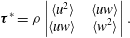
These two parameters were calculated in a similar way by Ge et al. (Reference Ge, Dasi, Sotiropoulos and Yoganathan2008).
Calculated from spatial velocity derivatives,
 $\unicode[STIX]{x1D70F}_{max}$
was very sensitive to the grid resolution of the measurements; if the grid was too coarse, the smallest structures of the flow would not be resolved and the viscous shear stress would be underestimated; however, if the grid resolution was too fine, the calculated velocity would contain erroneous noise and result in an overestimation of the viscous shear stress. To reduce the error in the calculated shear stress caused by such noise, a Gaussian filter (using a
 $3\times 3$
window) was applied to the vector fields, which was found by Luff et al. (Reference Luff, Drouillard, Rompage, Linne and Hertzberg1999) to be able to reduce the average uncertainty of second-order calculations from PIV data from
 $\pm$
37 % to
 $\pm$
4 %.
A grid refinement test was performed for measurements made in both the axisymmetric and anatomical models. For the axisymmetric model, the interrogation window was set at 12
 $\times$
12 pixels, which resulted in acceptably low levels of noise in instantaneous velocity measurements with a spatial resolution of
 $105~\unicode[STIX]{x03BC}\text{m}$
. For the anatomical model, however, the interrogation window had to be increased to 24
 $\times$
24 pixels, which corresponded to a spatial resolution of
 $270~\unicode[STIX]{x03BC}\text{m}$
. It was reasoned that the viscous stress calculated for the anatomical measurements would be somewhat underestimated as a result of the relatively low resolution. To correct for this, a corrective mapping algorithm was derived from the results in the axisymmetric model and applied to the viscous stress measurements in the anatomical model. Details of the grid refinement test as well as the derivation of the corrective mapping algorithm can be found in appendix A.
4 Flow loop validation: axisymmetric model
The flow conditions generated by the flow loop were validated by comparing measurements taken in the axisymmetric test section to similar ones reported by previous authors. Velocity measurements were made at the peak flow phase, on the plane perpendicular to the valve’s symmetry plane. The profiles of the phase-averaged axial velocity
 $\langle W\rangle$
and root-mean-square velocity fluctuations
 $w^{\prime }$
are compared in figure 7 with profiles by Yun et al. (Reference Yun, Dasi, Aidun and Yoganathan2014a
), obtained numerically with the entropic lattice-Boltzmann method and by Dasi et al. (Reference Dasi, Ge, Simon, Sotiropoulos and Yoganathan2007), obtained with PIV, for position
 $z/D_{i}=0.234$
downstream of the valve (
 $D_{i}=21.4$
mm for both previous studies). The velocities were normalized by the average velocity
 $W_{0}$
of the corresponding profile (
 $W_{0}=1.012~\text{m}~\text{s}^{-1}$
for the present study and
 $0.720~\text{m}~\text{s}^{-1}$
, for both previous studies).
The shapes of the jet profiles were nearly identical, although the normalized peak jet velocities of the present study were on average 8 % higher, and the central jet was more rounded than that of Yun et al. (Reference Yun, Dasi, Aidun and Yoganathan2014a
). The normalized velocity fluctuations were also in very good agreement with those reported by Yun et al. (Reference Yun, Dasi, Aidun and Yoganathan2014a
) in both shape and magnitude. The largest discrepancy was of the fluctuations on the outer shear layer of the
 $x^{-}$
jet, with the values in the present study being larger by 31 %. Overall, the mean and root-mean-square velocities showed excellent agreement with other measurements under comparable conditions, which inspires confidence in the results presented herein.
Phase-averaged (a) and root-mean-square fluctuations (b) of axial velocity at peak flow, and at
 $z/D_{i}=0.234$
in the axisymmetric channel, compared with similar measurements by Yun et al. (Reference Yun, Dasi, Aidun and Yoganathan2014a
) and by Dasi et al. (Reference Dasi, Ge, Simon, Sotiropoulos and Yoganathan2007).

5 Velocity maps in the anatomical aorta model
Before presenting the results for the anatomical model, it seems necessary to provide some explanations concerning technical limitations that where encountered due to the complexity of and small imperfections in the apparatus.
-
(a) A circular area in the
$y$
–
$z$
field, located at the top of the non-coronary sinus was masked from viewing because this area was optically blocked by the right coronary artery inlet. -
(b) A small triangular-shaped area in the
$y$
–
$z$
field, located at the bottom of the
$y^{+}$
side wall was also masked from viewing. This was necessary because of the optical obstruction caused by a small section of the silicone insert that was made to model the aortic root geometry; this insert fit seamlessly to the interior of the aorta base for most of its perimeter, but protruded slightly into the channel at this masked-out location. It is believed that this protrusion had insignificant effects on the flow patterns. -
(c) Some imperfections in the anatomical model, such as inhomogeneities in the silicone, caused some streaks to appear in the calculated velocity field. To minimize this artefact, the vectors were calculated using a 24
$\times$
24 pixel interrogation window, rather than the 12
$\times$
12 pixel interrogation window used for the measurements in the axisymmetric model.


To illustrate the flow past the valve within the complete aorta geometry, the phase-averaged velocity measured at phase C for the normal valve orientation is shown in figure 8 for the
 $y$
–
 $z$
and
 $x$
–
 $z$
centreplanes. The images are composites of multiple fields of view (three for the
 $x$
–
 $z$
plane and two for the
 $y$
–
 $z$
plane), which were measured independently and collated in post-processing.
Phase-averaged planar velocity magnitude
 $q_{pl}$
in the anatomical model for the normal valve orientation at peak flow (phase C), for the
 $y$
–
 $z$
(left) and
 $x$
–
 $z$
(right) centreplanes. NC – non-coronary sinus; RC – right coronary sinus; LC – left coronary sinus.

In agreement with previous descriptions of BMHV flows, the triple jet was found to dominate the flow field and recirculation vortices formed in the sinuses. For this valve orientation, the
 $x$
–
 $z$
plane depicts the cross-sections of the three jets, whereas the
 $y$
–
 $z$
plane shows the cross-section of the central jet. Unlike in the axisymmetric model, the triple jets were not symmetric about the
 $z$
-axis (
 $x=0$
) (figure 8, right). The jet nearest the convex wall of the aorta propagated the furthest of the three, while the one nearest the concave wall jet propagated the shortest distance and impinged on the outer wall of the aorta, just past the end of the right coronary sinus. This asymmetry was consistent with previous studies of flow in the aorta, which found that velocities in the ascending aorta during systole were higher toward the convex wall than the concave wall (Klipstein et al.
Reference Klipstein, Firmin, Underwood, Rees and Longmore1987; Chandran Reference Chandran1993).
The sinus geometry in the
 $y$
–
 $z$
plane was strongly asymmetric about the
 $z$
-axis: the non-coronary sinus was located in the
 $y^{-}$
side of the root, but there was no sinus opposite it. As a result, a large recirculation vortex formed in the non-coronary sinus and a much smaller recirculation vortex formed on the other side (figure 8). This effect was propagated upwards into the ascending aorta, where a low velocity region existed next to the
 $y^{-}$
wall, but not at the
 $y^{+}$
wall. In fact, a second jet formed at the
 $y^{+}$
wall resulting in a double-peaked velocity profile. This is illustrated in the inset of figure 8, which shows the axial velocity profile at
 $z/D=1.55$
(section A–A).
6 Effects of valve orientation on the velocity field and the fluid stresses
6.1 Planar velocity maps
Phase-averaged velocity
 $q_{xz}$
on the
 $x$
–
 $z$
centreplane at phases B (a,c,e) and C (b,d,f), for normal (a,b), aligned (c,d) and inclined (e,f) valve orientations. Red dashed lines indicate the
 $x$
–
 $z$
centreplane, viewed from downstream.

The phase-averaged velocity maps on the
 $x$
–
 $z$
centreplane at mid-acceleration (phase B) and peak flow (phase C) are shown in figure 9 for the three valve orientations.
For the normal valve orientation, the
 $x$
–
 $z$
plane shows the three jets (see also figure 8), which at mid-acceleration (phase B) extended into the aortic root. At this phase, the lateral jets were more developed and stronger than the central jet and their axes were inclined towards the sinus walls, with the lateral jet on the
 $x^{+}$
side deflecting off the channel wall above the sinus; recirculation vortices are seen to form between the lateral jets and the sinus walls.
For the aligned valve orientation, the
 $x$
–
 $z$
plane was parallel to the valve symmetry plane and contained the profile of the central jet. At mid-acceleration, this jet was seen to emerge past the valve leaflets into the aortic root. The velocity in the sinuses was very low – lower than the value for the normal orientation at this phase. At peak flow (phase C), the profile of the central jet was very narrow. Its axis was aligned with the
 $z$
-axis up to approximately
 $z/D=1.25$
, beyond which it curved slightly following the aorta curvature. At this location, a second velocity peak, lower in magnitude than the peak of the central jet, formed near the concave channel wall. This double-peaked profile was similar to the one that developed past the valve on the
 $y$
–
 $z$
plane for the normal orientation, as seen in figure 8.
For the inclined valve orientation, the
 $x$
–
 $z$
centreplane was oblique to the valve symmetry plane and its central orifice and intersected the corners of the valve’s lateral orifices, as illustrated by figure 6(c). The flow issuing from these corners is shown on the
 $x$
–
 $z$
plane as the narrower, shorter jets located on either side of the central jet profile (figure 9).
Phase-averaged axial velocity profiles on the
 $x$
–
 $z$
centreplane at (a)
 $z/D=0.65$
and (b)
 $z/D=1.60$
for normal, inclined and aligned valve orientations at peak flow.

Figure 10 shows profiles of the mean axial velocity
 $\langle W\rangle$
in the
 $x$
-direction for the three valve orientations at
 $z/D=0.65$
and 1.60. The profiles at
 $z/D=0.65$
, which was approximately two-thirds down the length of the sinus, reveal that, for all three valve orientations, the reverse velocity in the right coronary sinus (on the
 $x^{-}$
side) was much stronger than in the left coronary sinus. Because this asymmetry appears to be independent of valve orientation, it is likely caused by the aorta curvature or other asymmetries in the anatomical geometry. The aligned valve orientation did, however, result in slightly stronger reverse flow in the left sinus, compared to the two other orientations. Further downstream, at
 $z/D=1.60$
, the triple jets of the normal orientation were less pronounced than at
 $z/D=0.65$
, as they merged and spread; they were also slightly skewed toward the
 $x^{-}$
side as a result of the aorta’s curving toward the opposite direction.
The phase-averaged velocity maps for the three valve orientations on the
 $y$
–
 $z$
centreplane at phases B and C are shown in figure 11. As was shown in figure 8, the
 $y$
–
 $z$
centreplane contained the cross-section of the central jet for the normal orientation. For the aligned valve orientation, the
 $y$
–
 $z$
plane intersects all three jets. At phase B for this orientation, the lateral jet on the
 $y^{+}$
side appears to be deflected off of the channel wall as was observed for the normal valve orientation at the same phase (as shown by the
 $x$
–
 $z$
plane in figure 9). At phase C, the axes of the three jets were aligned with the
 $z$
-axis and all jets appeared to be symmetric.
For the inclined orientation, the map on the
 $y$
–
 $z$
plane shows oblique cross-sections of the three jets, which were similar to those shown for the aligned orientation on this plane. In contrast to the velocity maps on the
 $x$
–
 $z$
plane for this orientation, in which the central jet was relatively wide and the lateral jets were very narrow, the jet profiles on the
 $y$
–
 $z$
plane were all comparable in width.
At mid-acceleration, the recirculating flow in the non-coronary sinus was stronger for the aligned and inclined orientations, where it was adjacent to the lateral jets, than for the normal orientation, where it was adjacent to the central jet. This pattern, however, was reversed at peak flow, when the sinus flow was stronger for the normal orientation than for the two other orientations.
Phase-averaged velocity
 $q_{yz}$
on the
 $y$
–
 $z$
centreplane at phases B (a,c,e) and C (b,d,f) for normal (a,b), aligned (c,d) and inclined (e,f) valve orientations. A circular area located at the top of the non-coronary sinus was masked from viewing because this area was optically blocked by the right coronary artery, which exited the model there.

6.2 Turbulent stress
The maximum turbulent stress
 $\unicode[STIX]{x1D70F}_{max}^{\ast }$
is shown in figure 12 for the three valve orientations at peak flow on the
 $x$
–
 $z$
and
 $y$
–
 $z$
centreplanes. In general, regions of high turbulent stress occurred at the outer edges of the lateral jets and, to a lesser degree, between the lateral jets and the central jet (shown in planes perpendicular to the valve symmetry plane) as well as at the sides of the central jet (shown in planes parallel to the valve symmetry plane).
For each valve orientation, average values of
 $\unicode[STIX]{x1D70F}_{max}^{\ast }$
at peak flow were calculated by taking into account the measurements on both the
 $x$
–
 $z$
and
 $y$
–
 $z$
planes within the ranges
 $z/D=0.2$
to 1.5,
 $x/D=-0.8$
to 0.83 (
 $x$
–
 $z$
planes) and
 $y/D=-0.85$
to 0.7 (
 $y$
–
 $z$
planes). The average value for the normal valve orientation was 21 % higher than for the aligned one (18.5 Pa versus 15.3 Pa). The average value for the inclined orientation was 16.9 Pa, however, because the measurement planes were not orthogonal to the valve’s symmetry as was the case for the two other orientations, the turbulent stress levels for the inclined orientation cannot not be compared directly to those for the normal and aligned orientations.
Turbulent stress
 $\unicode[STIX]{x1D70F}_{max}^{\ast }$
at peak flow for valve orientations: normal (a,b), aligned (c,d) and inclined (e,f), in the
 $x$
–
 $z$
centreplane (a,c,e) and the
 $y$
–
 $z$
centreplane (b,d,f). Red arrows connect the planes that were perpendicular to the valve’s symmetry plane and the planes that were parallel to it. The region for the inclined orientation marked with cross-hatching was believed to be strongly affected by error, attributed to loss of optical access, and was not considered in the analysis.

More specifically, the turbulent stress in the direction perpendicular to the valve’s symmetry plane was higher for the normal than for the aligned orientation at the outer edges of the lateral jets, with the corresponding peak value being 10 % higher (92 Pa versus 84 Pa). These regions of relatively high stress were also somewhat more extensive for the normal orientation. The more significant increase in turbulent stress for the normal orientation compared to the aligned one, however, was on planes parallel to the valve’s symmetry plane at the edges of the central jet and, even more so, in the spaces between the central jet and the channel walls.
For the inclined valve orientation, two streaks with relatively high turbulent stress levels are shown on the
 $x$
–
 $z$
plane. These streaks corresponded to flow emerging from the corners of the valve’s lateral orifices. The turbulent stress in these regions was even higher than that at the outer edges of the lateral jets for the normal orientation (peak values of 205 Pa versus 92 Pa). Both streaks extended to the end of the sinuses. The high stress level in these streaks is attributed to separation from the valve housing and the leaflets, which were very close together on this plane.
Averaged
 $\unicode[STIX]{x1D70F}_{max}$
at peak flow for valve orientations: normal (a,b), aligned (c,d) and inclined (e,f), in the
 $x$
–
 $z$
centreplane (a,c,e) and the
 $y$
–
 $z$
centreplane (b,d,f). Red arrows connect the planes that were perpendicular to the valve’s symmetry plane and the planes that were parallel to it.

Measurements near the base of the aortic root just past the valve on the
 $y$
–
 $z$
plane for the inclined orientation are believed to be strongly affected by error, attributed to loss of optical access, and therefore will not be considered in the analysis. The
 $y$
–
 $z$
plane reveals a turbulent stress distribution similar to that measured for the aligned orientation on the same plane, but the stresses were slightly lower: excluding the masked region, the average and peak stresses were, respectively, 16 % and 25 % lower than those for the aligned orientation.
6.3 Viscous shear stress
Figure 13 shows the phase-averaged viscous shear stress
 $\unicode[STIX]{x1D70F}_{max}$
at peak flow for the three valve orientations on the
 $x$
–
 $z$
and
 $y$
–
 $z$
centreplanes. Normal to the valve’s plane of symmetry (the
 $x$
–
 $z$
plane for the normal orientation and the
 $y$
–
 $z$
plane for the aligned orientation), high levels of viscous shear stress existed at the shear layers of the jets; such shear layers formed between the lateral jets and the valve housing, between the lateral jets and the valve leaflets and between the central jet and the leaflets.
To show the distributions of the instantaneous levels of shear stress, histograms were generated from the instantaneous measurements for both the normal and aligned valve orientations. The measurements from both the
 $x$
–
 $z$
and
 $y$
–
 $z$
centreplanes were used to generate the histogram for each orientation, which was then normalized by the area beneath them to obtain the probability density function (PDF), denoted
 $f(\unicode[STIX]{x1D70F}_{max})$
. It has been previously shown that viscous shear stress values as low as 10 Pa can cause damage to platelets (Ge et al.
Reference Ge, Dasi, Sotiropoulos and Yoganathan2008). The PDFs, shown in figure 14, indicate that shear stress levels exceeding this threshold occurred more frequently for the normal valve orientation than for the aligned one; the percentages of measurements that exceeded 10 Pa were 1.7 % and 1.3 % for the normal and aligned valve orientations, respectively.
Normalized histogram of
 $\unicode[STIX]{x1D70F}_{max}$
for normal and aligned valve orientations from the
 $x$
–
 $z$
and
 $y$
–
 $z$
centreplanes (a) with a zoomed-in view about the threshold for platelet damage (b).

A PDF was not made for the inclined valve orientation because, as was explained for the turbulent stress measurements, the measurement planes were not orthogonal to the valve’s symmetry as was the case for the other two orientations, thereby making a direct comparison of the results inappropriate.
Maps of phase-averaged viscous shear stress (figure 13) indicate that the viscous stress was higher for the normal orientation than for the aligned orientations on planes both perpendicular and parallel to the valve’s symmetry plane. Perpendicular to the valve’s symmetry plane the peak shear stress level at the base of the shear layers was 7 % higher for the normal orientation than for the aligned orientation (8.8 Pa versus 8.2 Pa).
From the maps of phase-averaged viscous shear stress for the inclined orientation (figure 13), streaks of high viscous shear stress were shown on the
 $x$
–
 $z$
centreplane, corresponding to the flow emitted from the corners of the lateral orifices. These stresses, however, were not as high as at the outer shear layers of the lateral jets, shown on planes normal to the valve symmetry plane. In other words, the flow from these corners exhibited extremely high levels of turbulence and moderately high levels of viscous shear stress.
7 Effects of valve orientation on flow in the right coronary artery
Figure 15 shows phase-averaged planar ‘streamlines’ (namely, lines that are tangent to the planar velocity vectors) in the
 $x$
–
 $z$
plane at three time instances during flow acceleration and peak flow for the three valve orientations. At
 $t/T=0.086$
, for all orientations, the flow was in the forward direction and fluid entered the coronary artery. For the normal valve orientation, the
 $x^{-}$
lateral jet appeared to be mid-way into the aortic root, whereas for the aligned and inclined orientations, no jets were visible. In the normal orientation, the sinus recirculation vortex formed between the lateral jet and the sinus wall, but it was small and did not seem to influence the coronary flow.
Phase-averaged planar ‘streamlines’ of flow in the right coronary artery for two phases during acceleration (
 $t/T=0.086$
– (a–c) and
 $t/T=0.108$
– (d–f)) and at peak flow (
 $t/T=0.214$
– (g–h)) for normal (a,d,g), aligned (b,e,h) and inclined (c,f,i) valve orientations.

At
 $t/T=0.108$
, the central jet extended into the root for the aligned and inclined orientations, and the sinus vortex formed between the root and the sinus wall. Recall that this vortex is the cross-section of a three-dimensional vortex ring that occupies the space next to the wall around the channel’s perimeter. In the right sinus, the vortex at this time was larger for the inclined than the aligned orientation, extending further towards the channel centre. The velocity in the coronary artery was higher than at the previous phase for the aligned and inclined orientations, and, of all orientations, was highest for the aligned one. For the normal orientation, the sinus vortex was further downstream than at the previous phase and extended past the opening of the coronary artery. Flow from the lateral jet was wrapped around the vortex while entering the artery.
At
 $t/T=0.214$
(peak flow) and for all orientations, the sinus vortex occupied the entire sinus region and blocked flow from entering the coronary artery. A second vortex may be seen to form inside the artery, which is evidence of flow recirculation.
Figure 16 shows planar streamlines for the three valve orientations at three time instances during flow deceleration. Slightly after peak flow, at
 $t/T=0.261$
, the flow in the aorta decelerated and, for all orientations, the sinus vortices retreated slightly upstream of its previous location, partially unblocking the coronary ostium, so that flow again wrapped around the vortex and entered the artery. As the fluid was diverted around the vortex, it entered the artery at an inclination to the artery’s axis. As a result, in all orientations, the flow separated at the downstream-side entrance to the artery, and the forward coronary flow was confined to the upstream side of the vessel. The area of separation was smaller for the inclined valve orientation, where the flow entered the vessel in a direction that was in closer alignment with its axis. Additionally, the sinus vortex occupied a larger region of the sinus for the inclined orientation than for the others, and included flow nearer the channel centre. The phase-averaged centre of vortex recirculation for this orientation was located further upstream than for the other orientations; it was located the furthest downstream for the normal valve orientation.
Phase-averaged planar ‘streamlines’ of flow in the right coronary artery for decelerating phases
 $t/T=0.261$
(a–c) and
 $t/T=0.314$
(d–f), and
 $t/T=0.364$
(g–i) for normal (a,d,g), aligned (b,e,h) and inclined (c,f,i) valve orientations.

At
 $t/T=0.314$
, for the aligned and inclined orientations, forward flow continued to enter the coronary artery; however, for the normal orientation, the artery became blocked again by the sinus vortex, causing flow to cease in the artery.
At
 $t/T=0.364$
, for all valve orientations, the sinus vortex was located slightly inward toward the channel centre, and reverse flow drained from the artery in the area between the vortex and the sinus wall. Velocity maps taken at other time instances, which are not shown here for the sake of economy, revealed that the reverse coronary flow began at an earlier phase for the normal orientation than for the other two. At
 $t/T=0.364$
, the reverse flow was strong for this orientation, and a second vortex formed between the drainage jet and the sinus wall. The sinus vortex was confined between the drainage jet and the lateral jet coming from the BMHV. For the aligned and inclined orientations, at
 $t/T=0.364$
, the drainage flow was weaker and followed the sinus wall. Maps at later time instances, also not shown here, demonstrated that the drainage flow for these orientations was strengthened and that a second vortex formed between the drainage jet and the sinus wall, like that shown for the normal orientation at
 $t/T=0.364$
.
The bulk flow rate in the right coronary artery was estimated by integrating the velocity in the direction of the artery axis (
 $V_{RC}$
) across the channel, under the assumption that the arterial flow was axisymmetric. The detailed procedures used for this calculation have been described by Haya (Reference Haya2015). Figure 17 shows the axial velocity
 $V_{RC}$
determined across a diameter near the artery’s inlet during flow acceleration (
 $t/T=0.086$
).
Radial direction in the right coronary artery (a) along which the phase-averaged variation of axial velocity
 $V_{RC}$
is shown (b) at
 $t/T=0.086$
for the aligned valve orientation.

The resulting bulk flow rates for the three valve orientations are plotted in figure 18. This figure shows that the majority of coronary flow occurred at two times during the forward part of the cycle: around mid-acceleration and around mid-deceleration. For all three valve orientations, the coronary flow rate was near zero around peak flow due to the blockage of the ostium by the sinus vortex. Positive coronary flow resumed during deceleration, when the sinus vortex retreated slightly upstream, partially unblocking the coronary ostium. The vortex blocked the ostium for a second time during late deceleration, again reducing coronary flow, before moving inwards towards the channel, thus allowing reverse flow to drain from the coronary artery.
During flow acceleration, the coronary flow rate was greatest for the aligned valve orientation and lowest for the normal orientation. During deceleration, however, the coronary flow was greatest for the inclined orientation and lowest for the aligned orientation. The volume of fluid that entered the coronary artery was estimated by integrating the flow rate over the duration of forward coronary flow for each orientation. This volume was lowest for the normal orientation (0.74 mL), slightly greater for the aligned orientation (0.84 mL) and greatest for the inclined orientation (1.2 mL).
(a) Phase-averaged flow rate in the aorta during the forward flow phase of the cycle; key phases are indicated by letters as: A – start of systole; B – mid-acceleration point; C – peak of the forward flow; D – mid-deceleration point; E – peak reverse flow, and F – valve closure. (b) Phase-averaged flow rate in the right coronary artery during the forward flow phase of the cycle for normal, aligned and inclined valve orientations.

8 Analysis of the results and discussion
8.1 Effects of valve orientation on flow distribution
It was found that, on the
 $x$
–
 $z$
centreplane, the reverse flow in the left coronary sinus was greater for the aligned valve orientation than for the normal and inclined orientations. This may be because in the normal orientation the lateral jets spread outward into the sinuses, leaving less room for recirculation. Comparatively, in the aligned orientation the valve’s central orifice was roughly adjacent to the left sinus – the central jet was narrower than the lateral jets and left more room for sinus recirculation.
From the measurements on the
 $y$
–
 $z$
plane for the normal orientation, it was shown that the low velocity region of the non-coronary sinus extended far into the ascending aorta. In vivo, this non-physiological low flow region could foster thrombus growth by increasing the contact time between potentially activated platelets and proteins involved in coagulation. Furthermore, by altering the viscous shear stress distribution at the adjacent vessel walls, it may promote arterial disease (Paszkowiak & Dardik Reference Paszkowiak and Dardik2003). For the aligned and inclined orientations, however, the field of view was limited to the aortic root and did not include the ascending aorta. As a result, it was not possible to determine the extent of the low velocity region for these valve orientations. It was interesting to note, however, that the velocity in the non-coronary sinus was even lower for both of these orientations than for the normal one. One may postulate that, because the lateral velocity components of the three jets were very small at peak flow, the low flow region would extend fairly deeply into the ascending aorta. As was shown in figures 9 and 11, however, the fluid velocities near the channel walls were typically higher on planes perpendicular than on planes parallel to the valve’s plane of symmetry, due to the spread of the lateral jets. As a result, the low velocity region (measured on the
 $y$
–
 $z$
centreplane) would not likely extend as far for the aligned and inclined orientations as it did for the normal valve orientation.
8.2 Effects of valve orientation on turbulent and viscous stresses
The turbulent stresses were on average 21 % higher for the normal valve orientation than for the aligned orientation. Additionally, the normal valve orientation resulted in 31 % more occurrences of viscous shear stresses that were high enough to potentially activate platelets. These results suggest that the aligned orientation may be preferable over the normal one from the viewpoint of minimizing the stresses acting on blood elements, and reducing the potential for thrombosis.
The previous suggestion is in contrast with the conclusion of Borazjani et al. (Reference Borazjani, Ge and Sotiropoulos2010) that the valve orientation had no significant effect on the viscous shear stress downstream of the valve. These authors, however, also recommended the aligned orientation, but on the grounds that it resulted in the most synchronous valve closure and lowest leaflet rebound, which they attributed to the near uniformity of pressure on the leaflets for the aligned orientation; for other orientations, the two leaflets were unequally affected by the pressure gradient imposed by the aorta curvature. Borazjani et al. (Reference Borazjani, Ge and Sotiropoulos2010) also postulated that the aligned configuration would be less susceptible to intermittent regurgitation.
Kleine et al. (Reference Kleine, Perthel, Nygaard, Hansen, Paulsen, Riis and Laas1998) found that, from measurements made in two pigs, the Reynolds normal stresses were lowest when a BMHV was oriented with one lateral orifice toward either the posterior wall or the right-posterior wall of the aorta; these orientations were close to, respectively, the aligned and inclined orientations of the present study. This result was fairly consistent with that of the present study.
It would be of interest to compare these findings with clinical outcomes for varying BMHV orientations, however, to our knowledge, such data have not yet been published. Furthermore, thromboembolic rates may be a poor indicator of valve performance, because they can be highly influenced by patient risk factors and antithrombotic management (Sotiropoulos et al. Reference Sotiropoulos, Le and Gilmanov2016).
Figure 12 shows that the largest differences in turbulent stress for the two orientations occurred in the shear layers in the wake of the valve housing. Specifically, the turbulent stress at the outside edge of the
 $x^{-}$
lateral jet in the normal orientation was much higher and extended over a larger area than in any of the shear layers for the aligned orientation. This was likely a consequence of the lateral jet impingement on the concave wall. Conversely, when the valve was in the aligned orientation, there was more space between the jets and the concave wall, and the jets did not impinge on it.
Another significant difference in the turbulent stresses was shown on the valve symmetry plane: in the normal orientation, high levels of turbulent stress developed in the space between the central jet and the non-coronary sinus (on the
 $y$
–
 $z$
centreplane). This did not occur for the aligned orientation, for which the turbulent stresses were very low on the valve symmetry plane (the
 $x$
–
 $z$
centreplane). Figure 19 shows the velocity projections on the valve symmetry planes for the normal and aligned orientations at peak flow and
 $z/D=0.40$
. For the normal orientation, the velocity profile on the
 $y^{-}$
side of the central jet protruded, forming a local velocity peak between the central jet and the reverse flow in the non-coronary sinus. This resulted in a steep velocity gradient between this protrusion and the reverse flow, which increased the production of turbulence there. In the aligned orientation, on the other hand, the velocity transition between the central jet and the reverse sinus flows was much more gradual. The asymmetric protrusion of the velocity profile observed for the normal orientation may have resulted from the asymmetry of the sinuses with respect to the central jet on the valve symmetry plane. In contrast, for the aligned orientation, the channel walls of the left and right sinuses were nearly symmetric about the central jet profile.
Velocity projections on the planes parallel to the valve symmetry plane for normal (orange arrows) and aligned (blue arrows) valve orientations at peak flow and
 $z/D=0.40$
; as a scale for velocity magnitudes, the figure shows a black arrow with a length equivalent to
 $1~\text{m}~\text{s}^{-1}$
.

Coronary artery disease has been found to be an appreciable cause of morbidity following aortic valve replacement, while 34 % of patients having valve replacement for aortic valve stenosis also have significant coronary artery disease (Exadactylos, Sugrue & Oakley Reference Exadactylos, Sugrue and Oakley1984). Previous studies have found that the formation and development of atherosclerotic plaques can be predicted by deviations in the physiological patterns of wall shear stress; specifically, complex flows that result in low level or oscillating wall shear stress have been found to be pro-atherogenic (Gibson et al. Reference Gibson, Diaz, Kandarpa, Sacks, Pasternak, Sandor, Feldman and Stone1993; Friedman, Krams & Chandran Reference Friedman, Krams and Chandran2010). Such flows, which can be found in bifurcating and curved arteries (Friedman et al. Reference Friedman, Krams and Chandran2010), may also occur in the flow separation region observed at the downstream side of the right coronary ostium. To reduce the risk of plaque formation there, it is desirable to decrease the size and duration of this flow separation. The area of flow separation appeared largest for the normal valve orientation and smallest for the inclined valve orientation, indicating that the inclined orientation would cause the least risk for plaque development there.
8.3 Effects of valve orientation on right coronary flow
As was previously documented (Yoganathan, He & Jones Reference Yoganathan, He and Jones2004), the lateral jets emerged earlier than the central jet during flow acceleration. This was also apparent when comparing the coronary flows on the
 $x$
–
 $z$
plane for the different valve orientations (figure 15). Consequently, the portion of the sinus vortex that was adjacent to the lateral jet advanced earlier than the portion that was adjacent to the central jet. As a result, when a lateral valve orifice was oriented toward the coronary artery (i.e. in the normal orientation), the sinus vortex blocked the coronary ostium earlier than for the other valve orientations. This caused the coronary flow rate during flow acceleration to be much lower than for the other orientations.
Sketch of inferred vortex ring shape without the effects of valve orientation.

At mid-acceleration, the aligned orientation resulted in the highest coronary flow rate. In addition to the delayed advance of the sinus vortex, the coronary flow for this orientation was augmented by the high velocity fluid of the jet adjacent to it, part of which rolled over the sinus vortex into the artery. For the inclined orientation, the coronary flow also benefited from the delayed sinus vortex; however, the adjacent fluid emitted from the valve was not as fast and, consequently, the coronary flow rate was slightly lower than for the aligned orientation.
During flow deceleration, the coronary flow was highest for the inclined valve orientation. This appears to have been a direct result of the size, shape and orientation of the sinus vortex. For both the normal and aligned orientations, the sinus vortex next to the coronary ostium was confined by the adjacent lateral jet, which was aligned with the axial direction. For the inclined orientation, however, the fluid velocity in the aortic root had a significant transverse component directed away from the coronary ostium. As a result, the sinus vortex was confined by a lesser amount, and it entrained more fluid from the channel centre. Additionally, this caused the long axis of the vortex to be inclined more than for the other orientations, which permitted the fluid from it that entered the coronary artery to be more in line with the artery’s axis. Consequently, there was a weaker flow separation at the artery entrance, and a larger portion of the artery contained forward moving fluid.
The measurements presented here reveal information about the three-dimensional shape and time evolution of the sinus vortex ring. The vortex had a larger cross-sectional diameter on the
 $x$
–
 $z$
plane at
 $y/D=0.165$
, where the right coronary sinus was deepest, than on the
 $x$
–
 $z$
centreplane, which did not extend as far into the sinus. This was expected as it is presumed that the vortex would occupy the space between the valve housing and the channel wall, which is larger in the depths of each sinus than at the commissures between them. We can infer that the sinus ring would therefore be thicker in all three sinuses and thinner at the locations between them, taking on a trimodal shape similar to the perimeter of the aortic root. This inferred shape is depicted in figure 20. The cross-sectional diameter of the sinus ring was further affected by the valve geometry; it was larger in parts that were adjacent to the central orifice than in parts that were adjacent to the lateral orifices, where it was confined by the outward-spreading lateral jets. The largest vortex ring diameter was thus achieved when the valve’s line of symmetry was in line with the right coronary ostium (namely, the inclined orientation); in this orientation the portion of the vortex ring located within the right sinus was also adjacent to the valve’s central orifice. As we saw in § 7, this configuration resulted in the largest forward flow volume in the contiguous right coronary artery. Furthermore, the measurements illustrated that the sinus ring was advected downstream earlier in parts adjacent to the lateral orifices than parts adjacent to the central orifice. This would likely cause the trimodal-shaped ring to bend in a ‘V-shape’ about the valve’s plane of symmetry, in a fashion similar to the one reported by Dasi et al. (Reference Dasi, Ge, Simon, Sotiropoulos and Yoganathan2007).
It must be noted that the results from the measurements of coronary flow have limited relevance to physiological conditions. In vivo, the majority of coronary flow occurs during diastole, because the contraction of the heart during systole compresses the coronary arteries, increasing their flow resistance. During diastole, while the bulk flow rate in the aorta is nearly zero, the heart muscle is relaxed and the coronary arteries dilate, causing blood to flow through them, a process made possible by arterial compliance which serves as a flow reserve. This effect was not accounted for in the present mock circulatory apparatus; to do so, an active, timed resistance would have had to be applied at the outlets of the coronary arteries, which would have been considerably difficult to implement in our set-up and so has been deferred to a specific future investigation. Because in this study we applied a passive resistance that was constant over the course of the cycle, the majority of the coronary flow occurred during systole, rather than during diastole. The reverse flow in the coronaries at the end of systole may be attributed to the local adverse pressure gradient that builds up at this time. This reverse flow would likely have been accentuated by imperfect sealing of the BMHV during valve closure (Dasi et al. Reference Dasi, Murphy, Glezer and Yoganathan2008), which would expose the fluid at the coronary inlets to the suction upstream of the valve. Moreover, gravity may have likely contributed to the draining of the coronaries, as our model was oriented such that the anatomical frontal plane was vertical.
Despite this limitation, our work has provided some useful and novel information. First, we have confirmed that the size, shape and space–time evolution of the vortex ring depends strongly on BMHV orientation, and described details of this dependence. Moreover, we have demonstrated that, in the absence of intramyocardial pressure, the coronary flow rate depends strongly on the size, shape and space–time evolution of the sinus vortex ring. These observations may be considered towards predicting the dependence of coronary flow on BMHV orientation when physiological, time-varying resistances are imposed. We may plausibly assume that, even when subjected to physiological resistance, the sinus vortex would still have some, albeit somewhat lessened, influence on the coronary flow. The present results reveal the complex interactions between the flow in the aortic root with those in the coronary arteries without the added effect of vascular resistance caused by intramyocardial pressure. They provide a first step in understanding the physiological flow interactions and may be used in future studies, which account for the time-varying vascular resistance, as a basis for comparison in order to understand those effects. Such studies with more realistic coronary flow are being considered for future work.
Although the flow rate in the left coronary artery was not measured, it may be presumed that the inclined valve orientation, which was optimal for the right coronary flow, would not be optimal for the flow in the left coronary artery. When the valve’s symmetry plane is aligned with the right coronary ostium (i.e. for the inclined orientation), one of the valve’s lateral orifices would be positioned next to the left coronary ostium – for the right coronary artery, this arrangement resulted in the lowest coronary flow rate. One may then speculate that the aligned valve orientation would be optimal for the total flow in both coronary arteries; this suggestion may be justified by the facts that the aligned orientation resulted in the second highest right coronary flow rate (after the inclined orientation), and a symmetric positioning of the ostia with respect to the valve symmetry plane, which means that the right and left arterial flows would be equally affected. This hypothesis is supported by the centreplane velocity measurements presented in § 6.1, which showed that the aligned orientation resulted in the strongest reverse flow in the left coronary sinus (figure 10) and consequently the strongest left coronary flow. In case, however, the flow in one coronary artery was for some reason deficient, it could potentially be boosted by implantation of the valve so that its symmetry plane would be aligned with the axis of that artery.
Kleine et al. (Reference Kleine, Scherer, Abdel-Rahman, Klesius, Ackermann and Moritz2002) found, in contrast, that the flow in the left coronary artery of pigs was highest when the BMHV was oriented with one lateral orifice toward the right coronary cusp. This orientation was comparable to our ‘normal’ orientation which resulted in the lowest right coronary flow, but may have positioned the central orifice towards the left coronary, which would be consistent with the present findings. This shows further evidence of a need to test the effect of BMHV orientation on the flows in both coronary arteries simultaneously. Furthermore, an analysis of clinical outcomes for varying BMHV orientations from a large patient sample would be valuable for validating these findings.
9 Summary
The flow characteristics past a BMHV in an anatomical model of the aorta under physiological flow conditions were measured and analysed for three valve orientations. First, we investigated the effect of valve orientation on the velocity field and the turbulent and viscous stresses past the valve. Second, we investigated the effect of valve orientation on the flow rate in the right coronary artery.
It was found that, at peak flow, the turbulent stresses were on average 21 % higher and viscous stresses higher than 10 Pa (namely of a level that has been associated with blood cell damage) were 30 % more frequent when the valve was oriented with its plane of symmetry normal to the aorta’s plane of curvature, than when it was parallel to it. This was attributed to the impingement of a lateral jet on the concave wall of the aorta and to steeper velocity gradients resulting from the geometrical imbalance of the sinuses relative to the valve’s central jet when the valve was in the normal orientation.
For the inclined valve orientation, very high turbulent stresses and moderately high viscous shear stresses were found to occur in the shear layers that were generated from the corners of the valve’s lateral orifices. The turbulent stress level here was higher than that measured at any location for the other two valve orientations, but one is reminded that measurements near the corners were only possible for the inclined valve orientation.
Velocity profiles across the right coronary artery were measured for the three valve orientations, and the bulk flow rate through the coronary was calculated for the forward flow phase. For all valve orientations, the majority of coronary flow occurred at the mid-acceleration and the mid-deceleration phases of the flow cycle. The coronary flow rate substantially decreased at peak flow, as the result of blockage of the coronary ostium by the sinus vortex. The flow rate through the artery was highest for the inclined valve orientation and lowest for the normal orientation, for which the sinus vortex was advected downstream and blocked the coronary ostium earlier than for the two other orientations. For the inclined orientation, the sinus vortex extended further into the channel centre, drawing more fluid into the coronary. Additionally, the vortex axis was aligned better with the coronary axis and the resulting flow separation region was smaller. It should be noted, however, that the present experimental set-up could not account for the compliance and the time-varying resistance of the coronary arteries.
As a summary of the main results of the present work, table 2 lists the average and peak turbulent stresses and the percentages of viscous stress measurements that exceeded 10 Pa for the
 $x$
–
 $z$
and
 $y$
–
 $z$
centreplanes and for the combined measurements on both planes. The same table also lists the average forward flow volumes per cycle measured in the right coronary artery for the three valve orientations.
Summary of main results for the three valve orientations. The plane-averaged and the plane-maximum values of
 $\unicode[STIX]{x1D70F}_{max}^{\ast }$
are, respectively, shown outside and inside parentheses.

In closing, it is noted that the results of this study were obtained for a specific aorta geometry, and that there may be some variation in the flow characteristics as the result of anatomical differences among persons. We expect that, although minor differences in the flow patterns would inevitably be patient specific, the general findings would be applicable to all patients. For example, positioning the valve normal to the aorta’s curvature would likely result in jet impingement and the associated increase in fluid stresses and aligning the central orifice of the valve with a coronary ostium would result in the sinus vortex being larger next to the ostium, thus allowing more fluid to enter the coronary. We also note that the presently used rigid model of the aorta lacked the compliance of the natural aorta, which would likely affect the flow characteristics. A study of these effects is needed, but was beyond the scope of the present work.
Instantaneous axial velocity
 $W$
at
 $z/D=0.35$
, during phase B, in the axisymmetric model, calculated in four different ways: (i) using an
 $8\times 8$
pixel final interrogation window size, (ii) as in (i) but with a Gaussian filter applied, (iii) using a
 $12\times 12$
pixel final interrogation window size and (iv) as in (iii) but with a Gaussian filter applied.

This research adds to the knowledge base that may assist surgeons in choosing the best implantation orientation for a BMHV. We found that fluid stresses were lower when the valve was positioned with its plane of symmetry aligned with the aorta curvature than for other valve orientations. We also found that the highest flow rate in the right coronary artery occurred when the valve was aligned with the corresponding ostium and predicted that the highest total coronary flow would occur for the same valve orientation; a more conclusive study of coronary flows will hopefully be undertaken in the near future in a modified mock circulation loop, which would permit the modelling of more physiological coronary flow conditions.
Acknowledgements
Financial support by the Natural Sciences and Engineering Research Council of Canada (NSERC) is gratefully acknowledged. The bileaflet heart valve was kindly donated by St Jude Medical, Inc.
Appendix A. Viscous shear stress calculation from planar velocity measurements
A.1 Grid refinement test
Figure 21 illustrates the effects of final interrogation window size and the Gaussian filter on the calculated velocity. An axial velocity profile from the axisymmetric model was plotted for one instant during phase B of the cycle (mid-acceleration), having been calculated in four different ways: (i) using an
 $8\times 8$
pixel final interrogation window size, (ii) as in (i) but with a Gaussian filter applied, (iii) using a
 $12\times 12$
pixel final interrogation window size and (iv) as in (iii) but with a Gaussian filter applied. The flow at this mid-acceleration phase has been previously described as laminar and repeatable (Dasi et al.
Reference Dasi, Ge, Simon, Sotiropoulos and Yoganathan2007; de Tullio et al.
Reference de Tullio, Cristallo, Balaras and Verzicco2009), so the velocity profile should not exhibit turbulent fluctuations, and any fluctuation observed in the profile could be considered to be noise. The level of noise for both of the
 $8\times 8$
window size cases and for the
 $12\times 12$
unfiltered case was unacceptably high and would have introduced artificially high velocity gradients that would have resulted in a significant overestimation of the viscous shear stress, but the
 $12\times 12$
window size with the Gaussian filter resulted in acceptably low levels of noise; therefore these conditions were used for the calculation of the axisymmetric vector fields. The test was repeated for the measurements in the anatomical model and a
 $24\times 24$
pixel window size was deemed appropriate.
Viscous shear stress mapping algorithm: (a)
 $\unicode[STIX]{x1D70F}_{max12}$
calculated from 12
 $\times$
12 pixel interrogation windows; (b)
 $\unicode[STIX]{x1D70F}_{max24}$
calculated from 24
 $\times$
24 pixel interrogation windows; (c) scaling factor versus
 $\unicode[STIX]{x1D70F}_{max24}$
and fitted polynomial; (d) corrected
 $\unicode[STIX]{x1D70F}_{max}$
mapped from
 $\unicode[STIX]{x1D70F}_{max24}$
.

A.2 Corrective mapping algorithm
Figure 22 shows a comparison between the phase-averaged viscous shear stresses that were computed in two ways: (i) from a 12
 $\times$
12 pixel interrogation window, denoted as
 $\unicode[STIX]{x1D70F}_{max12}$
(figure 22
a); and (ii) from a 24
 $\times$
24 pixel interrogation window, denoted as
 $\unicode[STIX]{x1D70F}_{max24}$
(figure 22
b). It is clear that
 $\unicode[STIX]{x1D70F}_{max24}$
was much lower than
 $\unicode[STIX]{x1D70F}_{max12}$
. In view of the fact that the noise for the vectors calculated with the 12
 $\times$
12 pixel interrogation window was quite low, the underprediction of
 $\unicode[STIX]{x1D70F}_{max24}$
was attributed to the relative coarseness of the grid, which did not permit the capturing of small-scale fluctuations in the flow.
It can be reasoned, then, that the viscous shear stress calculated using a 24
 $\times$
24 pixel interrogation window size for the anatomical measurements would also be underestimated. To correct for this, a corrective mapping algorithm was derived from the results in the axisymmetric model.
Inspection of the quotient of
 $\unicode[STIX]{x1D70F}_{max12}$
and
 $\unicode[STIX]{x1D70F}_{max24}$
revealed that it was not constant, but larger for lower values of
 $\unicode[STIX]{x1D70F}_{max}$
and smaller for larger values of
 $\unicode[STIX]{x1D70F}_{max}$
. To compensate for this variation, the quotients were sorted into bins corresponding to values of
 $\unicode[STIX]{x1D70F}_{max24}$
, and an average scaling factor for each range of
 $\unicode[STIX]{x1D70F}_{max24}$
was calculated; this has been plotted in figure 22(c). A polynomial fitted to the results was used to determine the appropriate scaling factors for correcting measured values of
 $\unicode[STIX]{x1D70F}_{max24}$
. As a test, it was applied to
 $\unicode[STIX]{x1D70F}_{max24}$
from the axisymmetric model to obtain a corrected measure of
 $\unicode[STIX]{x1D70F}_{max}$
(figure 22
d). This corrected shear stress, mapped from the larger grid data, is nearly identical to that calculated directly from the finer grid. This polynomial was used to correct measurements made in the anatomical model processed with a 24
 $\times$
24 pixel interrogation window.



