

1 Introduction
The standard justification for benefit–cost analysis (BCA) is the potential compensation test (PCT).Footnote 1 This paper makes the point that the PCT is not the proper justification for the use of BCA and is also unsatisfactory as the rule for accepting a project (Chipman & Moore, Reference Chipman and J. C1978). As a result, I suggest dropping the PCT along with its significant deficiencies. Instead, a proper justification for use of BCA is based directly on the Pareto justification, known as the Consent Justification, suggested by Edgeworth in the nineteenth century (1891). This article furnishes the present-day support for its use. The Consent Justification is the Pareto test by which no one, or almost no one, loses. The consent rationale I suggest is that the use of BCA is justified if all tend to gain. With a strong tendency for all to gain, it is reasonable to assume that people would approach unanimity in agreeing to the general use of the technique, especially in an original position. On a project level, projects should be accepted simply when they have positive net present value (NPV), which is, in fact, the measure used in practice.Footnote 2 These conclusions of using a better justification (consent) and dropping the PCT are reached by examining the PCT more carefully by a simulation exercise showing a high probability that all gain from the use of BCA when considered across a portfolio of projects.
2 Problems with the potential compensation test
Over time, it has become apparent that the PCT contains sources of appropriate criticisms and also deficiencies.Footnote 3 These are the following: (i) it is not used or needed, (ii) it lacks moral appeal being based on hypothetical, and often impossible, transfers, (iii) it is subjected to Scitovsky reversals, and (iv) it fails in legal cases, of which there are many, where the sum of expectations exceeds the value of the project. Indeed, Chipman and Moore (Reference Chipman and J. C1978, p. 581) in a trenchant article have noted that in fact with respect to hypothetical compensation and other justifications, “When all is said and done, the New Welfare Economics has succeeded in replacing the utilitarian smoke-screen by a still thicker and more terrifying smoke-screen of its own.”
2.1 Not used
In a survey of over 300 BCAs, I do not find one that uses the PCT. Nor, to the best of my knowledge, has anyone been able to point out a project in which the PCT is used. The reason is clear, using PCT is difficult and expensive. One would need to determine both the compensating variation (CV) and the equivalent variation (EV) for each project and there would be some projects that pass one test but not the other, so there would be indeterminacy. A common assumption is that a positive NPV implies that the PCT is passed. Yet, this is untrue (Boadway & Bruce, Reference Boadway and Bruce1984). It might be thought that for small projects or price changes, the CV and EV would be similar, as income effects could be small, so that the CV alone is a reasonable approximation. Yet, even for small projects, with small income effects, the differences can be quite large, as Knetsch (Reference Knetsch1989) and others have shown, due to endowment effects.
Similarly, it might be thought that if the PCT is not used, there is no point in arguing, as I do here, for its abandonment. There are at least three reasons to reject this view. First, some believe that a project that passes the NPV test means that it also passes the PCT, but this is untrue and should be clarified. Second, it seems important to have the scientific foundations of BCA theory clearly stated, which is not now the case currently. Third, the PCT is the source of substantial criticism.
2.2 Lack of moral appeal
A Consent Justification is more appealing than one based on hypothetical compensation. This is shown by the numerous articles, spanning many years of law, economics, and philosophy literature, whose criticisms of cost–benefit analysis (CBA) are mainly addressed to the use of the PCT.Footnote 4 (For a sampling, see Anderson, Reference Anderson1993, Ackerman & Heinzerling, Reference Ackerman and Heinzerling2002; Ackerman & Heinzerling, Reference Ackerman and Heinzerling2005; Chipman and Moore (Reference Chipman and J. C1978); Heinzerling, Reference Heinzerling2002; Heinzerling, Reference Heinzerling1998; Richardson, Reference Richardson2000; Sagoff, Reference Sagoff1988).Footnote 5 This tension and these misunderstandings are illustrated in the 2007 exchange between Steven Kelman and several others (Kelman, Reference Kelman1981 in Delong et al. and in Goulder (Reference Goulder2007). The use of PCT suggested ty Kaldor is historically associated with Kaldor’s (Reference Kaldor1939) injunction to avoid moral sentiments in the use of CBA.Footnote 6 Moral goods for which there is a willingness to pay are economic goods as are any others. To exclude them, even in theory, is inconsistent with foundational economics. It is worth noting that the use of costless hypothetical compensation has led McConnel1 et al. (Reference McConnell1997) to a major error in assessing the use of moral sentiments (Zerbe et al., Reference Zerbe, Y and A2006a).
Second, the PCT lacks moral standing, as it rests on the notion of purely hypothetical compensation. Actual compensation is not required and could not necessarily, and probably not usually, be carried out if compensation costs are considered.Footnote 7 In any empirical setting, if policymakers actually sought to compensate project losers, the costs associated with identifying losers, ascertaining losses, and implementing compensation (not to mention likely litigation costs) would be very expensive, even to the point at which any net gains would disappear (Zerbe & Knott, Reference Zerbe, Knott and J2004, p. 431). Thus, projects that pass the PCT often would not, in practice, be able to compensate losers.
2.3 Use in legal dispute
Baker (Reference Baker1979) observes that the PCT is not useful in most legal cases, even though a considerable body of literature holds that BCA is a mainstay of common law and other law in the sense that judges use BCA reasoning in making new law. Baker points out that in lawsuits it is usual that the sum of parties’ expectations regarding the ownership of a legal right (or good) exceeds the actual value of the legal right. In such cases, the PCT cannot be satisfied regardless of who wins the case. Baker considers a situation in which persons A and B each believe with 80 % probability that the value of some property right is theirs. If the value of the good in question is $100, and goes to person A at law, person A gains $20 and person B loses $80 – and vice versa, so that no matter who wins, the other cannot, even potentially, be compensated. Baker concludes on this basis that the use of the PCT criterion is not useful for these sorts of legal cases. The NPV is not subject to this objection as the property goes to whomever has the highest NPV (Zerbe, Reference Zerbe2014).
2.4 Scitovsky reversals
Scitovsky (Reference Scitovsky1941) introduced a dual criterion to replace the sum of compensating variations proposed by Kaldor and known as the Kaldor–Hicks (KH) criterion. KH states that a project is desirable if the winners are able, in the original state of the world, to hypothetically bribe the potential losers to undertake the project. The Hicks (Reference Hicks1939) test is that the losers are not able to hypothetically bribe the winners to not undertake the project. Scitovsky notes that using KH, it is possible to recommend a move from a state of the world, A, to a new one, B, and then having arrived at B, to recommend a move back from B to A. The dual tests of using both the compensating and equivalent variations would avoid this possibility known as the Scitovsky reversal paradox. The use of the dual criteria would, however, come at the expense of some indeterminacy when a project passes one test but not the other and at the considerable additional expense of determining both the EV and CV.Footnote 8
Some have seen the possibility of Scitovsky reversals creating a problem for the use of BCA. Adler and Posner (Reference Adler and E. A1999) correctly note that the possibility of such reversals haunt cost–benefit analysis. Coleman (Reference Coleman1988) goes further and claims that the possibility of inconsistent results arising from the Scitovsky paradox renders CBA impractical. On this basis, Coleman has held that CBA is incoherent or useless. Markovits (Reference Markovits1993) goes even further and claims that the possibility of such reversals renders all welfare economics’ arguments wrong. Elsewhere, Schmitz and Zerbe (Reference Schmitz and Zerbe2008) have shown that the technical arguments of Coleman and Markovits are incorrect, relying on second best situations.Footnote 9 The Posner and Alder comment remains germane to some extent. A definitive treatment is offered by Just et al. (Reference Just, A. and R2013). Reversal paradoxes such as Scitovsky’s are, however, purely creatures of the PCT, so without the PCT, there can be no reversals (Zerbe & Dively, Reference Zerbe and Dively1994, pp. 104–105). That is, there is no reversal paradox using NPV.
3 The Consent Justification
No perfect justification for valuation exists or can exist (Zerbe, Reference Zerbe2020; Talbott, 2020). Even the Pareto criterion has its critics. A reasonable justification, however, for BCA is consent. There are two kinds of consent, actual consent and consent in an original position.Footnote 10 Actual consent can be fairly assumed in so far as the use of BCA trends toward all persons gaining across a reasonably sized portfolio of projects. That is, some will lose from each project, but across all projects, all will tend to gain.
3.1 Conditions for consent
Clearly, when the total NPV across a portfolio of projects is positive, all will gain when (i) returns are proportionate to costs borne by each person, (ii) when the costs among persons are equal and returns are randomly distributed for a sufficiently large number of projects, or (iii) when costs for each person are less than their expected benefits. The second condition holds because a random distribution of project gains tends toward a uniform distribution as the number of projects increases. This is the law of large numbers. The first condition holds when, for example, benefits and costs from a public good are proportionally associated with the income of users. I define Ω to represent the higher of the three probabilities that one of these conditions holds. Thus, Ω will increase to the extent to which there is a political tendency toward equal taxation (equal costs) and random distribution of benefits or toward choosing projects in which gains are proportional to costs. As Ω increases, the probability that there are losers from P decreases toward zero. The Arrow–Lind theorem (Reference Arrow and Lind1970) shows conditions for which the social cost of the risk moves to zero as the population tends to infinity, so that projects can be evaluated on the basis of expected net benefit alone. A modified version of their proof shows that under the same conditions all tend to gain as net benefits increase aside from risk (Appendix B). Across a portfolio of projects sufficiently large, Ω will tend to be high even if costs are not equal.
4 The Consent Justification in a simulated framework
The appeal of the Consent Justification would be greatly enhanced if it was thought that the size of the relevant portfolio of projects needed to approach consent was not too large and was fairly robust to errors in BCAs. In order to examine how an application of the BCA might play out, I implement a simulation of the results using BCA in a world with a portfolio of projects for which there are net gains. For each project in a given simulation, the model calculates individual net benefit as a function of individual costs (taxes) and individual benefits (assigned via the project “winner” parameter and sampling function). Then as each additional project “occurs,” the model tracks the individual’s overall net benefit.
4.1 Initial model assumptions
(i). Only projects that pass a benefit–cost test are implemented: simply put, net present benefits must exceed net present costs for all projects.
(ii). All project costs and benefits are monetized: there are no nonmonetary costs associated with any and all projects, this assumption matters only to the degree that monetary and nonmonetary costs are not distributed equally.
(iii). Project benefits to individuals are uncorrelated across projects: receiving benefits from one project does not alter an individual’s likelihood of receiving benefits from another project.
(iv). Project benefits to individuals are independent of tax bracket: all individuals, regardless of tax bracket (i.e., cost burden), are equally likely to receive benefits from a given project (it is not assumed that the cost somebody bears is equal to the financing charge).
(v). Project costs are borne by all individuals in accordance with their designated tax bracket, while only those individuals sampled at random (from a uniform distribution) receive benefits from a given project.
(vi). The simulation assesses individual net benefit only as a function of taxes paid and public project benefits received, that is, “winners” are simply those who receive more in monetary benefits than they paid in taxes, and “losers” are those who pay more in taxes than they receive in monetary benefits.
(vii). All benefits and costs are immediate. Time is not incorporated in the model, thus, all effects occur instantaneously such that there is no inter-temporal discounting and project order does not matter.
4.2 Initial simulation
The model first selects a number of projects and a population size, each from a uniform distribution arbitrarily specified (1–100 projects and 100–100,000 people, respectively). Next, a project’s gross benefit figure is selected from a uniform distribution of $1000–100,000. While the magnitude of benefits can be varied by project, the mean value drives the model outcome, and so for the sake of simplicity, the benefit value is simply fixed. Project costs are randomly drawn from a uniform distribution with a lower bound of zero and an upper bound of project benefits minus $1 (thus satisfying Assumption 1). Note that the net benefit then varies by project. Next, we assign a figure for the proportion of individuals who receive benefits from the project, a “winners” parameter, this parameter, drawn from a uniform distribution of 0.01–1.00, represents the proportion of the population who receive project benefits. All individuals assigned to receive benefits receive an equal share (Project Benefits/(N × Proportion of Winners)). The proportion is fixed across a simulation but varies among simulations. The specific individuals from the population receiving project benefits are selected at random using a sampling function.
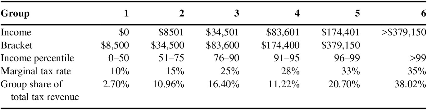
In order to allocate individual cost, the simulated population is divided into groups based upon the percentile rank associated with U.S. income tax brackets. These groupings are then matched to the proportion of total U.S. income taxes that are paid by individuals within this tax bracket. The simulated total project cost is then proportioned accordingly into each grouping, so that the individual cost is uniform within each group. These groupings are then matched to the proportion of total U.S. income taxes that are paid by individuals within this tax bracket. For the sake of simplicity, all individuals are assumed to be “single” in terms of tax status, thus, the rates below reflect the marginal tax rates for single filers on the 2011 U.S. Federal income tax. See Table 1 below.
The simulated total project cost is then proportioned accordingly into each grouping, and the individual cost is calculated by dividing this proportion by the number of people in each bracket (i.e., individual cost is uniform within each group). For each project in a given simulation, the model calculates individual net benefit as a function of individual costs (taxes) and individual benefits (assigned via the project “winner” parameter and sampling function). Then as each additional project “occurs,” the model tracks the individual’s overall net benefit as the cumulative sum of project-specific net benefits. The simulation outcome of interest is the proportion of individuals in the entire population who have positive net benefits after the “conclusion” of all projects in the simulation. This proportion reflects the number of people who are better off given the specified portfolio of projects. This simulation is then repeated 10,000 times, with different values for population size, project benefits, the “winners” parameter, and number of projects.Footnote 11
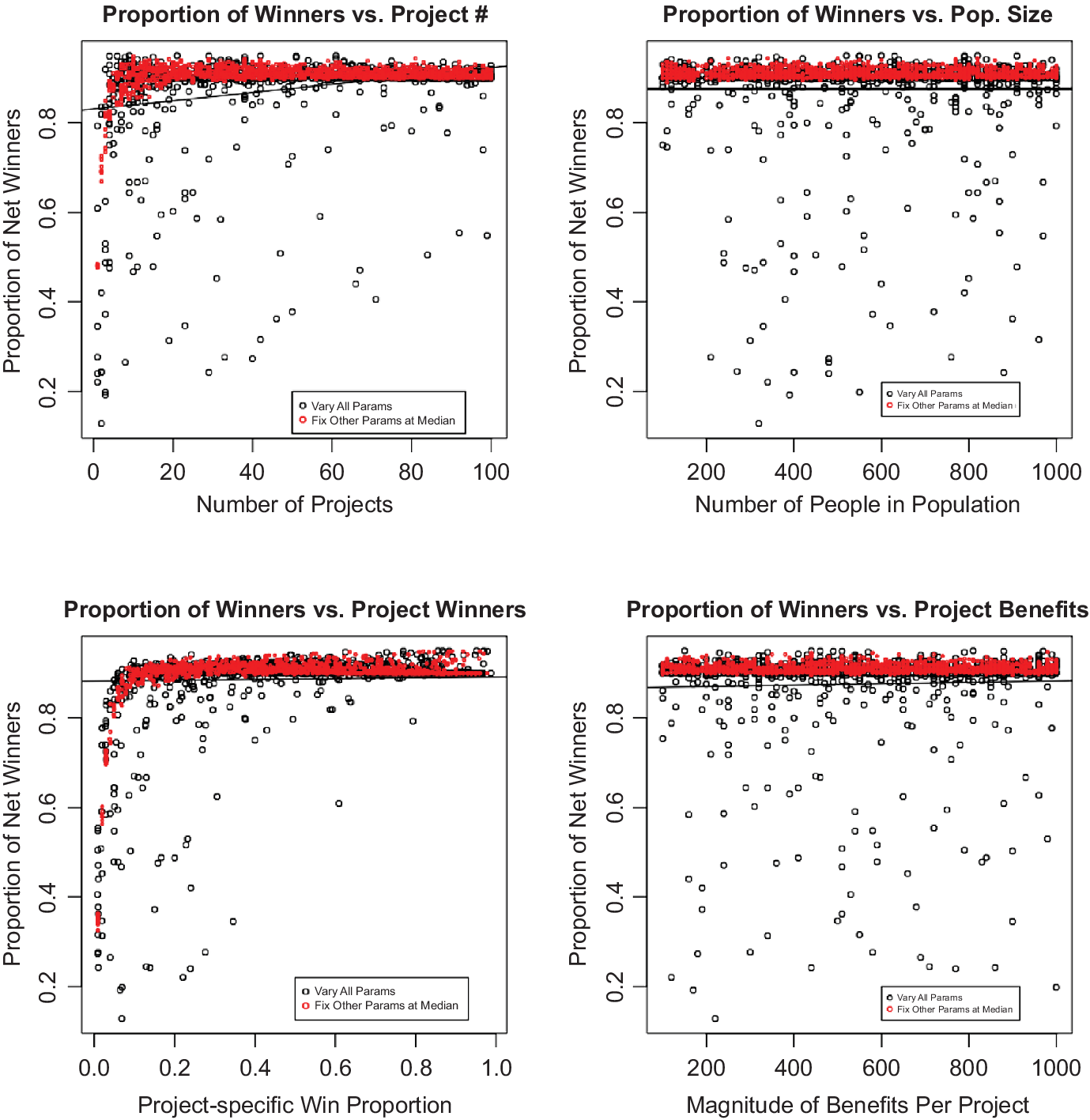
In the panels within Figure 1, the thin black line is the regression line. The red dots overlaid on the plot represent similar results, but for alternative simulations in which the three parameters not plotted on the x-axis are fixed at their median values (e.g., 50 projects). The results of these simulations are then plotted as the parameter along the x-axis varies. The results in Figure 1 demonstrate the isolated effect of the specified parameter. Each of the dots in the four plots in Figure 1 represent the result of one simulation with each plot showing the proportion of those with positive net benefits (y-axis) against the specified parameter value for that simulation (x-axis).
Tax data used to generate cost-bearing groups.

Sources: 2011 Federal income tax rates and 2009 summary of Federal income tax burden (Tax Foundation, www.taxfoundation.org).
Results of 1000 project portfolio simulations.

Mean overall proportion of individuals who end up with positive net benefits, effects of error rates.

As shown in the top left panel, we can see that the policy decision-making using a simple benefit–cost test results in approximately 90 % of the population receiving positive net benefits as the number of projects gets larger. What is striking about these results is that this 90 % figure is reached at a low number of projects (~20), and then does not materially increase further as the number of projects goes beyond 100. Finally, the bottom left panel shows how the simulation result varies given the prespecified parameter representing the proportion of the population who receive benefits from a given project in one simulation. For instance, if this parameter is set to 0.5, it means that 50 % of the population are chosen (via a simulated lottery) to receive benefits from a given project, the other half of the population receives no project benefits. The lottery is repeated for each project within the simulation.
While the variance decreases greatly as this parameter goes above 0.6, we see that most simulations result in approximately 90 % of the population receiving positive net benefits even at per-project benefit recipient parameter values as low as 0.1 (and for values of 0.3 or greater, no simulation results in less than 60 % of individuals being net winners). More importantly, we see that varying this parameter widely does not change the fundamental results.
The 90 % figure that most simulations reach demonstrates that the benefit–cost rule is rather robust to distributional issues (in that the presence of one or two projects in which benefits accrue primarily to a select few does not keep most individuals from coming out ahead). The 90 % level is a maximum limit in our simulations. This is due to the cost set-up. In this model, 10 % of the population (i.e., the top three tax brackets), pay about 70 % of all project costs. However, benefits are equally distributed across the population to those selected as project winners. As the proportion of costs borne by the top brackets falls, the proportion of winners goes to 100 %.
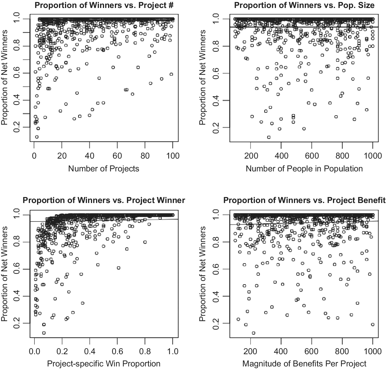
When we eliminate the tax bracket-based cost allocation function and instead assign costs uniformly across the population (such that the individual tax burden is simply Project Costs/N), the portion of winners also goes to 100 %. The results of these simulations are shown in Figure 2.
Cost allocated uniformly.

In addition, as benefits are distributed more according to costs borne, the results tend toward 100 %. In so far, as projects are based on willingness to pay, benefits may be expected to be positively correlated with income. See Frank (Reference Frank2000) and Gilens and Page (2014). For example, if a tax rate of 23 % is used across the top two quintiles, the model shows no losers, still at a low number of projects.
The simulations demonstrate the implications of using BCA without regard to potential compensation and the KH test. One can observe that, given certain assumptions about how project benefits are distributed (obviously, a not insignificant empirical issue), all individuals are likely to benefit so long as inefficient projects are not chosen, thus, the portfolio justification eliminates concern about the feasibility – and even possibility – of compensation, and rests on the estimated distribution of actual, instead of hypothetical, benefits and costs.
4.3 Error in BCA estimates (or choosing inefficient projects)
One particularly significant issue for any benefit–cost decision rule is that benefit–cost decision making is inherently an ex ante process. In other words, projects are selected because estimated benefits exceed estimated costs, with no guarantee that this predicted result will be borne out. Given the complexity of most policy decisions and the inherent uncertainty of complex systems, there is simply no way to avoid the possibility that a project might result in negative net benefits. This means, however, that negative outcomes should be assumed to occur. Even the best possible BCAs can prove erroneous, and thus it is important for a benefit–cost decision rule to be robust to this possibility, rather than simply “trying to do better” the next time. The following simulation explores how the portfolio approach performs under stochastic conditions in which project benefits do not necessarily exceed project costs.
Our initial model assumes that project benefits and costs are known with certainty, and that no project with negative net benefits will be selected. Of course, BCAs only estimate net benefits, and a lot can go wrong (or right) as a project unfolds over multiple years. Likewise, in selecting a portfolio of projects in practice, it is possible – if not likely – that policymakers will not elect to choose some projects that have positive net benefits and purposely choose some projects that have negative net benefits (perhaps for reasons of equity, security, etc.). Testing for this possibility is identical for testing for potential error in calculations, as either way the point of interest is the degree to which an actual portfolio can diverge from an idealized portfolio and yet still benefit almost everyone in the population.
In order to examine the robustness of our model to potential error in BCAs, we rework the cost function, this time randomly generating project costs along a shifted uniform distribution with a designated error rate. That is, we vary the mean of the cost distribution systematically, such that there is between a 1 % and 40 % probability that a given project actually produces negative net benefits. In reality, a 1 % error rate in identifying worthy projects is likely a bit low, while a 40 % rate is hopefully an extreme over-estimate. We assume that the magnitude of potential errors is in keeping with the magnitude of project estimates, so the error rate is reflected in terms of the potential for a benefit–cost ratio that is less than one.
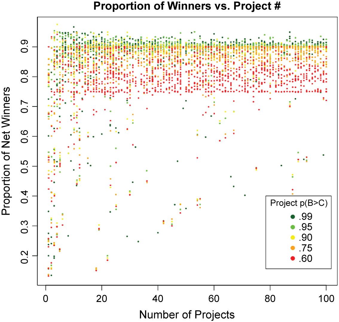
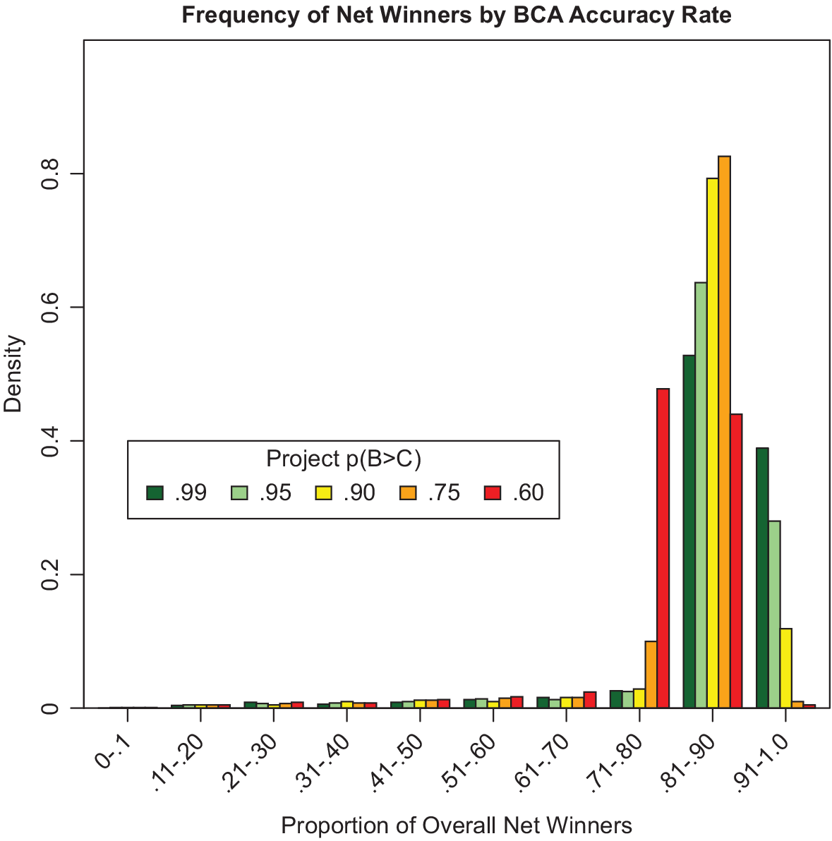
Figure 3 demonstrates simulation results given a 97.5, 95, 90, 75, and 60 % accuracy rate, respectively (with accuracy rate representing the probability that project benefits exceed project costs). Figure 3 demonstrates that even when we assume only a 60 % accuracy rate (i.e., a 60 % probability that a selected project has benefits that exceed project costs), in most cases at least 75 % of the population garners positive net benefits at the end of the simulation.
Scatter plot of net overall winners by accuracy rate.

Figure 4 shows the relative frequency of the probability of net overall winners (after the entire portfolio of projects). We can see that most observations find that at least 80 % of the population end up as net winners, and even at a 60 % BCA accuracy rate, almost all simulations result in at least 75 % of the population coming out as net winners.
Density of simulation net overall winners by accuracy rate.

4.4 Correlated benefits
Finally, we suppose that the recipients of benefits from public projects are not truly random. That is, one could hypothesize that particular individuals are adept at “gaming the system,” that political patronage greatly impacts the flow of benefits, or that receiving benefits from one project subsequently increases an individual’s ability to receive benefits from future projects. Political theory speaks to “increasing returns” and path dependence (e.g., Pierson, 2000; 2004).
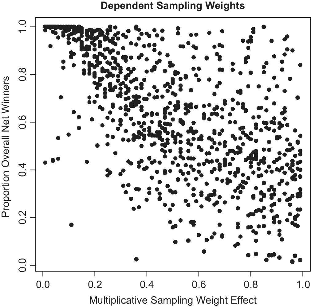
In short, how does “winning” on one project affect the distribution of winners on a subsequent project? To examine this, we utilize the same model as before, but now relax the third assumption (of uncorrelated project benefits) using a weighted sampling scheme. Figure shows the plot. In prior model iterations, all individuals were weighted equally such that each had an equal chance of being selected as a project winner (i.e., recipient of project benefits). Now, for one simulation (i.e., one portfolio of projects), we sample the winners for the first project from the entire population with uniform sample weighting, and then weight the population sampling of winners for project 2, according to whether or not an individual receives benefits from project 1.
For instance, if we use a weighting of 0.1, an individual who receives benefits from project 1 would have a sampling weight of 1 × 1.1 for project 2, and a project 1 “loser” would have a sample weight of 1 × 0.9. This sample weighting is then continued through the portfolio of projects (e.g., if an individual received benefits from both projects 1 and 2, the individual’s sample weighting for being selected as a benefit recipient of project 3 would be 1 × 1.1 × 1.1). Figure 5 demonstrates the results of a Monte Carlo simulation of 1000 project portfolios with a varying project winner correlation parameter (from 0.01 to 0.99).
Portfolio simulation with nonindependent sampling weights.

Note that we do not correlate project winners directly, but rather correlate the sampling weights such that the probability of winning from a future project is increased by winning on the current project, and the probability of winning from a future project is decreased by losing on the current project.
As expected, as the selection of project winners becomes less random (i.e., winning on one project more greatly influences probability of winning again), we see a decrease in the proportion of net overall winners in the population at the conclusion of the entire project portfolio. Empirically, we would not expect Assumption 3 to hold strictly, so a more relevant question is how strongly inter-project independence must be in order to approximate the results of strict independence. Figure 5 plots the proportion of individuals within the population who have positive net benefits at the end of the entire portfolio of projects against the value of the multiplicative sample weighting parameter used in each simulation run (using values from Previous Weight × 1.01 to Previous Weight × 1.99 for individuals who received benefits from the prior project).
For the simulations shown in Figure 5, BCA accuracy is set at 90 %, while project benefits, the number of projects, and per-project distributional benefits are varied. As shown by the Figure 5, as the distribution of individuals receiving benefits from any one project becomes less random (i.e., winning or losing on one project increases the probability of winning or losing on the next one), the proportion of overall net winners in the population trends downward. Note that as with the previous scatter plots, the overall distribution of points is most relevant to the question at hand. In a Monte Carlo simulation, many parameters are varied simultaneously, thus numerous outliers occur due to particular parameter combinations used in the model. In looking at such a plot then, one should be most concerned with: (i) the overall trend in Y as X changes and (ii) the variance in Y as X changes. The overall win proportion variance also greatly increases as the sampling weight adjustment parameter increases. Although at low levels (0.01 to ~0.30), the vast majority of model iterations result in a high proportion of net overall winners, as the sampling weight adjustment increases, the outcome variance also increases, such that the outcome of the portfolio becomes highly dependent on other contextual factors (e.g., whether projects have focused or highly diffuse benefits, as reflected by the per-project win proportion) and we cannot assume that the portfolio is likely to make everyone better off. Thus, if the assumption that benefits from one project are uncorrelated with benefits from any other project does not hold, the portfolio of BCA-approved projects cannot be assumed to be Pareto Relevant.
From a pragmatic standpoint, however, an important implication of Figure 5 is that at fairly small levels of inter-project correlation, we can be reasonably confident that a portfolio of projects will still result in a very high level of net overall winners. For simulations with weighting parameters less than 0.30, 60 % of the simulations result in at least 90 % of the population having positive net benefits at the conclusion of the portfolio. This figure rises to 78 % of simulations at parameter values less than 0.20, and 91 % of simulations at values less than 0.10.
4.5 Unequal weighting
One might reasonably hypothesize that the ability to influence the structure and selection of government policies is not uniform across the entire population. In other words, those in higher income brackets might be expected to be more effective at influencing government policies. Particularly, influence over government policies might facilitate a great deal of discretion over the spate of candidate projects that BCA is utilized to compare and select from, resulting in a “stacked deck” of possible projects. Moreover, it is reasonable to believe that there are more possible projects that help the richer than the poorer due to the higher willingness to pay (WTP) of the richer. In order to examine the implications of this possibility, we alter the sample weighting technique of the previous simulation by eliminating inter-project correlation for all individuals below the 90th percentile in income. Thus, the model assumes that receipt of project benefits is random for all individuals whose income falls below the 90th income percentile, while per-project benefits accruing to those earning above this threshold are assumed to be nonrandom.
It is perhaps doubtful that the rich are net losers from the use of BCA as compared with other income groups. There are reasons to believe that the benefits one realizes from public goods are likely to be positively correlated with one’s income. Amazon shareholders, for example, benefit greatly from the national infrastructure of roads, bridges, and broadband internet access. Beyond this general sort of correlation of benefits with income, CBA in practice is often based on willingness-to-pay measures, which Frank (Reference Frank2000), notes “virtually assures a mix of public programs that are slanted in favor of the preferences of high-income persons.” This point is also noted in almost every criticism of BCA (see Zerbe Jr., Reference Zerbe2007). As we note, the influence of special interest groups seems more, though of course not wholly, concentrated among the rich. Recently, Gilens and Page (2014) offer empirical evidence that the most powerful interest groups do exert significant influence on policy, and that their interests are usually not aligned with the common wellbeing. Nevertheless, it is quite possible and, we suspect, even likely, that the rich are still losers from the use of BCA as compared with most other political regimes for project selection.Footnote 12
There are several instances that might produce slightly different results than shown above. Where costs tend to be borne in proportion to benefits, the variance of net benefits is also reduced, and the results satisfy, or become close to satisfying (with project errors), the Pareto rule. Where taxes are higher for the wealthy, and their willingness-to-pay tends to be proportionally higher, the positive correlation reduces the variance of net benefits. This framework would tend to increase the equality of the income distribution. Individual projects can have highly concentrated benefits or highly concentrated costs.Footnote 13 A particular danger is that, when the less well-off bear significant costs, their willingness-to-pay is degraded for subsequent projects and a downward spiral result. By considering the effects over the range of projects, the portfolio, this danger may be ameliorated.
The portfolio approach can be a way of thinking about the justification for using BCA at all. It also can be used as an ex post guide about adjustments to future BCA projects, so as to provide winning projects to those who were losers previously. In this way, the possibility of actual compensation will be higher, all things being equal. Most important, however, a portfolio-based approach is meant to justify BCA as a governmental commitment to procedural fairness that, if applied consistently and in good faith, will ultimately increase social welfare and tend to not result in net losers. This simulation supports this possibility.
Finally, note that the substantive results of the simulation would not change if we were to simulate projects with different lifespans and cash-flow characteristics (e.g., front- or back-loaded costs or benefits). Our “timeless” model is functionally the same as if we were to apply a consistent discount rate for all individual’s benefits and costs, because all projects would still be subject to the assumption that policymakers are committed to selecting projects that pass a benefit–cost test. In other words, all projects are subject to the constraint that their net present value is positive, whether a project has a 50-year time horizon or whether all benefits and costs accrue instantaneously. If project cash flows are discounted by different methods and rates, then we can no longer be confident that the results shown above hold. This is really no different than the broader issue of consistent application of the BCA in policy selection.
5 Conclusions
I suggest that the Consent Justification be used as the rationale for BCA, rather than the KH criterion, the PCT. This suggestion is supported by a simulation that suggests all affected tend to be net winners across a portfolio of projects that satisfy a BCA test. This conclusion is rather robust to even relatively small portfolios of projects and the inclusion of even a significant number of projects that do not perform well. See Table 2 below. The case for the Consent Justification is strengthened by known deficiencies in the PCT, such as Scitovsky reversals, the failure to consider moral sentiments and the inability to perform when, as in legal cases, the total net value exceeds the expectations of the parties, as well as the fact that the PCT is rarely or never performed though often appealed to as the rationale for projects.
Acknowledgements
This project was aided by a grant from the MacArthur Foundation. I thank Tyler Scott for the simulations, Xu Tan and Michael J. Spackman for useful suggestions, Beatrice Bremer for copy editing, the referees who helped me make a more focused the argument, and Kole Kanter and Noel Hanzel for keeping my computer running during a difficult period.
Appendix A
It is well known that individuals may have differing time preference rates. Consider a social opportunity cost rate of 7 % and two people, A and B, with divergent time preference rates. A has a discount rate of 0 % and B a rate of 10 %. A project requires A and B to invest $100 each and will return $202 after 1 year to be split evenly among A and B. Thus, the project rate of return is 2%. A will have a net gain of $1.00 and B will have a net loss of $9.18. Net benefits are thus a negative $8.18. Yet it will always be possible ex ante to rearrange the burden of project costs and benefits so that both win by reducing costs to those with higher time preferences as long as one person has a time preference rate lower than the project’s rate of return. For example, if A costs are $180 and B’s are $10, one could split the returns so that A receives 190 and B receives 12, which means that each receives his rate of return and thus satisfies the PCT. Thus, the project can be made to pass the PCT even if the social rate of return is less than the opportunity cost rate.
More formally, Proposition 1: When hypothetical rearrangements of costs are allowed, as part of the PCT, which I will call a modified PCT, a project passes the PCT if at least one person has a time preference rate less than the government discount rate, R.
Proof: Assume at least one person has a time preference less than the social discount rate, R. Let a i be the fraction of costs borne by each individual, where the amount invested is X and is positive. The rate if return to the project is R *, which may be greater or less than R. which total future gross benefit is,
 $$ =X\left({e}^{R\ast t}\right). $$
There are ri rates of time preferences and n individuals. Let the share of each individual in the total return be ai. Let one rate of return, say r 1, be less than the rate R *. The sum of benefits allotted to each individual must satisfy their time preference rate so that equal the total return, that is:
 $$ \sum {a}_iX\kern0.5em {e}^{\mathrm{rit}}={Xe}^{R\ast }. $$
Each person gains or is indifferent if the ai coefficient is not less than zero. Positive, where a 1 + a 2 + … a n = 1.
Since r 1 < R *, for person 1 by definition, Proposition 1 is proved since that person will have some surplus and all the other shares of costs and benefits can be one. This would satisfy the PCT. It is also the case that all can gain regardless of their time preference rate as long as their share, that is, their ai is made sufficiently small while the share of a 1 is made sufficiently large. To show this, it is sufficient to note that Xe rt is a finite number as long as neither r nor t is finite. Any positive number, such as Xi e rt, can be made a vanishingly small number by making any ai sufficiently small.
Corollary 2: Proposition 1 holds even if NPV < 0. Let the value of the project be 𝑋𝑒R* < X𝑒𝑅𝑡.
As long as R * < R and one ri is less than R *, then the project is both inefficient and satisfies the modified PCT. Thus, an actual proposed project’s projected costs and benefits can be rearranged to pass the PCT even if it fails the NPV test as long as one person has a time preference rate less than the project’s rate of return.
Appendix B
The Many Projects Theorem: If the portfolio of projects is sufficiently large and the return Rj from the portfolio is positive, all will gain under some funding constraints.Footnote 14
The economy, contains a fixed number of persons, n. For simplicity, it is assumed that all n persons are affected by each project. Only projects with positive net present values are accepted. These projects taken together constitute P = {pi}, a portfolio of projects. All random variables have finite expectations. The portfolio can hold an infinite number of projects. The random variable xj(P) represents j’s income from current projects. The income from a new project is rj(p). These incomes are defined after all taxes and subsidies are taken into account so that rj represents the total impact of the project on j’s income. Let Z represent j’s total income, so that Z = ∑irj(pi). The value to j of projects are defined by expected values, Euj, of j’s utility function, which is strictly increasing continuously differentiable and finite. For a given project, j is better off by a given project if and only if,
 $$ 0<E\left\{ uj\left( xj+ rj\right)- uj(xj)\right\}. $$
Applying the mean value theorem to the expression under the expectation sign, and multiplying by P the condition becomes,
 $$ 0<E\left\{|P| rj\ {u}_j^{\prime}\left( xj+{\uptheta}_{\uptheta} rj\right)\right\}, $$
where θ j ranges from 0 to 1 (is an integrating factor).
Condition 1: for any given j as |P| → ∞, there are integrable limiting random variables R j and  $ {x}_j^n $ independent of one another, such that |P|rj → °R j and xj →
 $ {x}_j^n $.
Condition 1 clearly holds in the special case where rj(p) = Z(p)/n, where each persons’ income gain is equal. It is to be inferred from Condition 1 that rj(p) → 0 with probability one. This can be interpreted as showing that more valuable projects are selected first so that the return on the next project tends is lower. It follows that  $ {u}_j^{\prime } $(xj + θ jrj) →
 $ {u}_j^{\prime } $ (x n) since
 $ {u}_j^{\prime } $ is continuous. Condition 1 shows the expansion of Equation (5) for the increase in expected utility approaches Rj
 $ {u}_j^{\prime } $(
 $ {x}_j^n $) becomes E{Rj
 $ {u}_j^{\prime } $(
 $ {x}_j^n $)}. This equals ERjE
 $ {u}_j^{\prime } $(
 $ {x}_j^n $). Given the Rj and
 $ {u}_j^{\prime } $ (
 $ {x}_j^n $) are independent, as |P| → ∞ Equation (4) now becomes
 $$ 0\ \le\ ERj\ E{u}_j^{\prime}\left({x}_j^n\right), $$
or, since E  $ {u}_j^{\prime } $ (
 $ {x}_j^n $) is positive, more simply:
 $$ 0\ \le\ ERj. $$
Thus, when P is large, j is made better off from the project if, and only if the expected change in his income is positive. If, with Arrow and Lind, Rj = Z, which is invariant to |P|, then everyone is better off.