



1. Introduction
Frictional drag reduction technologies for marine vessels and underwater vehicles have long attracted considerable attention. Achieving lubrication of the external liquid flow for moving objects via gas injection constitutes a highly effective drag-reduction strategy (Ceccio Reference Ceccio2010), which can be broadly classified into three fundamental multiphase flow regimes: bubble drag reduction (BDR) (Kodama et al. Reference Kodama, Kakugawa, Takahashi and Kawashima2000; Kawashima et al. Reference Kawashima, Kodama, Hinatsu, Hori, Makino, Ohnawa, Takeshi, Sakoda, Kawashima and Matsuno2007), partial cavity drag reduction (PCDR) (Mäkiharju et al. Reference Mäkiharju, Elbing, Wiggins, Schinasi, Vanden-Broeck, Perlin, Dowling and Ceccio2013; Qin et al. Reference Qin, Sun, Fang, Wang, Chen and Wu2021) and air-layer drag reduction (ALDR) (Wu et al. Reference Wu, Ou and Ye2019a ; Wang et al. Reference Wang, Huang, Qin, Cao, Fang, Wu and Li2020; Mohamad et al. Reference Mohamad, Youssef, Bennaya and Elsherbiny2025). The underlying mechanism of drag reduction lies in the simultaneous reduction of the near-wall fluid density (Marié Reference Marié1987) and the solid–liquid wetted area (Fukuda et al. Reference Fukuda, Tokunaga, Nobunaga, Nakatani, Iwasaki and Kunitake2000) due to the presence of a stable air layer. Existing studies have demonstrated that ALDR exhibits the highest drag-reduction efficiency among the three approaches, reaching up to 60 %–90 % (Elbing et al. Reference Elbing, Mäkiharju, Wiggins, Perlin, Dowling and Ceccio2013), as ALDR serves as the most effective method to minimise solid–liquid contact. Extensive research efforts have thus been dedicated to the robust realisation of ALDR.
The methods of air-layer establishment can be categorised into two primary configurations: conventional gas injection through discrete orifices to form a near-wall air film (Kim & Steen Reference Kim and Steen2023), and the utilisation of ventilation slots combined with a backward-facing step (BFS) to separate the main flow from the wall, which was termed as the gas cavity method (Murai Reference Murai2014). Gas injection through orifices constitutes a classical jet-in-crossflow (JICF) problem. The dominant multiphase flow regimes in JICF typically manifest as discrete bubbles and a bifurcated cavity, strictly dictated by the injected gas volume flux
 $Q_j$
and the free-stream velocity
 $U_\infty$
(Xiong et al. Reference Xiong, Wang, Dong, Wang and Zhang2024). From the perspective of air-layer formation, buoyancy and surface tension may be crucial for multiphase hydrodynamics. Buoyancy drives the bubbles towards the solid boundary, facilitating their accumulation and coalescence into an air layer (Vigneau et al. Reference Vigneau, Pignoux, Carreau and Roger2001; Sanders et al. Reference Sanders, Winkel, Dowling, Perlin and Ceccio2006). However, under the buoyancy-driven regime of air-layer formation, Elbing et al. (Reference Elbing, Winkel, Lay, Ceccio, Dowling and Perlin2008) reported that a threshold gas flux as high as 2830 standard litres per minute (SLPM) was required to trigger the transition from bubbly flow to a continuous air layer in their experimental system. The ‘V’-shaped topology of bifurcated cavities was similarly governed by buoyancy, with a thin gas layer forming between the divergent cavity legs (Mäkiharju et al. Reference Mäkiharju, Lee, Filip, Maki and Ceccio2017). However, as elucidated by Mäkiharju & Ceccio (Reference Mäkiharju and Ceccio2018), when multi-point gas injection was employed for ALDR, the energetic barrier induced by surface tension between adjacent cavities (Eggers et al. Reference Eggers, Sprittles and Snoeijer2025; Hu et al. Reference Hu, Xu, Shi, Wang, Wang and Zhang2025) strictly inhibited spanwise coalescence, thereby leading to complex interfacial dynamics and unstable air layers.
The implementation of the gas cavity method serves as a strategic approach to facilitate the realisation of ALDR (Elbing et al. Reference Elbing, Mäkiharju, Wiggins, Perlin, Dowling and Ceccio2013; Zheng et al. Reference Zheng, Zhang, Tu, Xiong, Wang and Wang2025). Continuous spanwise uniform gas injection via ventilation slots, as opposed to orifices, enables the immediate formation of a nominally two-dimensional air layer, effectively circumventing the energetic barrier associated with bubble or cavity coalescence. Alternatively, passive flow control methodologies employing BFS (Karn et al. Reference Karn, Arndt and Hong2016; Zhang et al. Reference Zhang, Zhang, Sun and Jiang2023) artificially induce flow separation to facilitate air-layer formation, which has been proven effective by Qin et al. (Reference Qin, Wu, Wu and Hong2019). Nonetheless, a substantial critical gas flux was required as well. Below this threshold, the injected gas remained in the form of discrete bubbles within the recirculation region, which were subsequently entrained and transported downstream by the separated shear layer. Meanwhile, the critical gas flux is governed by the free-stream velocity (
 $U_\infty$
) and nominal cavity length (
 $l$
), and has been demonstrated to follow a scaling law with respect to the dimensionless parameter Reynolds number
 $\textit{Re}=\rho _l U_\infty l/\mu _l$
(Mäkiharju et al. Reference Mäkiharju, Elbing, Wiggins, Schinasi, Vanden-Broeck, Perlin, Dowling and Ceccio2013), where
 $\rho _l$
and
 $\mu _l$
denote the density and viscosity of liquid, respectively. The considerable injection gas fluxes fundamentally required for an air-layer establishment by these configurations may fail to deliver viable economic performance (Mäkiharju et al. Reference Mäkiharju, Perlin and Ceccio2012). From a practical standpoint, continuous ventilation slots inherently compromise the structural integrity of marine hulls.
Based on the discussions above, current ventilation strategies persistently struggle to simultaneously reconcile the requirement for lower gas fluxes with robust air-layer formation. The fundamental physical constraint arises from the intense gas entrainment induced by the high-momentum free stream. The spanwise spreading and coalescence are severely suppressed, with the gas being rapidly convected downstream as a bubbly flow rather than forming a continuous air layer. Recently, inspired by biological surfaces (e.g. lotus and Salvinia leaves) exhibiting extreme water repellency and self-cleaning capabilities, researchers have demonstrated that superhydrophobic (SHPo) surfaces facilitate rapid gas spreading, significantly curtailing the required gas flux for air-layer formation (Lee & Kim Reference Lee and Kim2011; Du et al. Reference Du, Wen, Zhang, Song, Ouahsine and Hu2017; Peifer et al. Reference Peifer, Callahan-Dudley and Mäkiharju2020; de la Cruz & Mäkiharju Reference de la Cruz and Mäkiharju2022). Furthermore, Xiang et al. (Reference Xiang, Huang, Huang, Dong, Cao, Li, Xue, Lv and Duan2020) elucidated that the microgrooves on Salvinia leaves motivate directional gas transport, enabling the generation of a global gas plastron via localised, low-rate gas injection. Thus, combining SHPo surfaces and transverse grooves that are oriented perpendicular to the flow direction may be favourable for modulating localised gas injection into a globally coherent air layer. Given that surface tension dominates the multiphase flow dynamics within these characteristic microstructures (Seo & Mani Reference Seo and Mani2016; Seo et al. Reference Seo, García-Mayoral and Mani2018; Sundin et al. Reference Sundin, Zaleski and Bagheri2021), the flow-modulation efficacy is intrinsically associated with the characteristic dimensions. The underlying size effect may therefore be imperative for the rational optimisation of multiphase flow control.
The establishment of a continuous air layer is governed not only by the interfacial dynamics, such as the coalescence of bubbles and the spreading of the air layer near the ventilation orifices, but also by gas leakage at the rear of the air layer. A stable air layer can only be established and develop downstream when the gas injection rate exceeds the leakage rate. This leakage process is, in turn, significantly modulated by the free-stream conditions. The interfacial instability arises from the substantial contrasts of density, viscosity and velocity between the gas and liquid phases (Spurk Reference Spurk2002; Wu et al. Reference Wu, Liu, Shao and Hong2019b ). Under specific flow conditions, an adverse pressure gradient induces an intense re-entrant flow that disrupts or precludes the downstream development of the air layer (Le et al. Reference Le, Franc and Michel1993; Wosnik et al. Reference Wosnik, Schauer and Arndt2003; Pelz et al. Reference Pelz, Keil and Groß2017). Concurrently, intense interfacial shear stress triggers Kelvin–Helmholtz (KH) instability (Michel Reference Michel1984; Funada & Joseph Reference Funada and Joseph2001; Kim & Moin Reference Kim and Moin2010). The subsequent advection of gravity–capillary waves along the gas–liquid interface is strongly correlated with gas leakage (Woods Reference Woods1966; Arndt et al. Reference Arndt, Hambleton, Kawakami and Amromin2009; Barbaca et al. Reference Barbaca, Pearce, Ganesh, Ceccio and Brandner2019). Consequently, the influence of these interfacial instabilities on the air-layer establishment within the current experimental configuration warrants a systematic re-examination.
This study experimentally investigates the modulation of multiphase flow by a transverse SHPo grooved surface across four distinct groove sizes and a range of free-stream velocities. The primary objectives are twofold: first, to elucidate the underlying physical mechanisms by which SHPo transverse grooves modulate the multiphase flow; and second, to delineate the parameter space of free-stream conditions and groove dimensions that defines the various air-layer regimes and their corresponding transition mechanisms. Accordingly, the paper is organised as follows. Section 2 describes the experimental facility and the parameter space explored. Abrupt multiphase flow regime transitions and the hydrodynamic pressure characteristics with and without modulation of SHPo transverse grooves are presented in § 3. Section 4 details the dynamic evolution of the air layer and its mechanical model. Section 5 characterises the three observed air-layer regimes and investigates the dependence of the macroscopic topology on free-stream conditions. Subsequently, the scaling laws governing the transitions between these regimes are established in § 6. Furthermore, the effects of ventilation flux and solid fraction on the air-layer regime transitions are examined in §§ 7 and 8, respectively. The drag-reduction performance achieved through the combined use of localised minimal ventilation and SHPo grooves is evaluated further in § 9. Finally, the conclusions are summarised in § 10.
2. Experimental facility and method
The experiment presented in this study was conducted in a gravity-driven circulating water tunnel. The experimental set-up primarily consisted of the water tunnel with a square test section measuring
 $100\,\text{mm} \times 100\,\text{mm}$
, a ventilation and control system, and an image and signal acquisition system. The ventilation and control system, comprising an air compressor, pressure-reducing valve, solenoid valve, micro-flow-control valve, and flow meter (
 $\pm$
1 % of full scale for fluxes below 2 SLPM) were connected in sequence, which was designed to enable precise control and measurement of the ventilation process. The image and signal acquisition systems were responsible for capturing the evolution of the ventilated air-layer morphology and recording pressure signals in the flow field. Two high-speed cameras (Phantom T2410) were positioned beneath the specimen and on its side, respectively, while two light-emitting diode (LED) lamps were strategically positioned to provide back lighting and front illumination. At the same time, high-resolution particle image velocimetry (PIV) was employed, and a laser sheet of approximately 0.5 mm thickness was generated to illuminate the tracer particles (Dantec FPP-RhB-10 1–20
 $\unicode {x03BC} \mathrm{m}$
) in the working fluid, enabling measurements of free-stream velocity upstream of the experimental specimen during each experiment. A detailed layout of the experimental set-up is shown in figure 1(a).
The experimental specimen was a flat-plate structure with a thickness of
 $D$
, incorporating a spherical–nose transition of radius
 $D$
at its upstream. Two ventilation orifices were arranged side by side with a spacing of
 $d$
. We fabricated the local SHPo transverse grooves with a square cross-section with characteristic sizes of
 $\delta =500,1000,1500\ \text{and}\ 2000\,{{\unicode[Arial]{x03BC}}{\rm m}}$
(dimensionless form
 $\delta ^*=\delta /D$
), which was coated with homemade superhydrophobic material (a layer of styrene–ethylene–butylene–styrene copolymer followed by the deposition of nanoparticles (Cao et al. Reference Cao, Liu, Zhang, Wu, You, Li, Duan, Huang and Lv2024; Zhang et al. Reference Zhang, Wan, Zhou, Cao, Duan, Yan, Li and Lv2024)). The scanning electron microscope images revealed that the SHPo materials exhibited a hierarchical surface morphology composed of microscale protrusions and nanoscale particles, as shown in figure 1(b). The contact angles of the coated surfaces were measured with a contact angle measurement apparatus, as shown in Appendix A. The multiphase fluid dynamic pressure was measured by three pressure transducers (supplied by PCB Piezotronics) with a sampling frequency set at 5000 Hz, which were arranged along the streamwise direction with a spacing of
 $2\hbox{-}\mathrm{D}$
. The detailed experimental parameters of geometry and flow conditions are noted in table 1.
The geometry and flow parameters for the experiments.

Table 1. Long description
The table presents the geometry and flow parameters for experiments. It has 11 rows and 3 columns. The columns are labeled Parameters, Symbol (unit), and Range. The parameters listed include specimen thickness, orifice radius, orifice spacing, ventilation gas flux, streamwise length of groove section, spanwise width of groove section, characteristic groove size, solid fraction, Reynolds number based on D, and Weber number based on delta. Each parameter is associated with a symbol and unit, followed by its range of values.
Schematic diagram of (a) the experimental set-up and (b) details of the experimental specimen, where the arrow represents the flow direction.

3. The transition from bubbly to air-layer flow under low ventilation gas flux
In this section, we will show two distinct flow regimes with and without the modulation of SHPo transverse grooves. A stable and continuous air layer can be established at a low ventilation gas flux through localised twin orifices. In addition, the pressure characteristics of the two multiphase flow regimes are also examined.
3.1. Morphology of bubbly and air-layer flow
Figure 2 illustrates two distinctly different flow states that emerge under nearly identical free-stream velocity and ventilation gas flux conditions, depending on whether the surface is smooth or equipped with SHPo transverse grooves. As shown in figure 2(a), for the smooth-surface case, the injected gas will go through the following successive stages: bubble growth, deformation, detachment and subsequent convection by the crossflow. This phenomenon occurs under conditions of low ventilation flux, where the injected gas is periodically pinched off by the free stream and forms discrete bubbles, a behaviour that has been reported by Xiong et al. (Reference Xiong, Wang, Dong, Wang and Zhang2024). The pinch-off event is governed by the competition between hydrodynamic forces and surface tension (Oguz & Prosperetti Reference Oguz and Prosperetti1993; Mirsandi et al. Reference Mirsandi, Smit, Kong, Baltussen, Peters and Kuipers2020). At relatively low ventilation flux, the injected gas expands slowly near orifices, leading to an increase in the hydrodynamic force exerted by the liquid crossflow. The hydrodynamic drag causes the air pocket to incline and elongate downstream, accompanied by the development of a local interfacial indentation. As the neck narrows, the increasing local curvature enhances the capillary pressure, eventually triggering neck collapse and pinch-off once it exceeds the local pressure difference across the interface. In contrast, figure 2(b) demonstrates the modulation effect introduced by the SHPo transverse grooves: a continuous air layer develops near the ventilation orifices and remains stable downstream, ultimately enveloping the entire surface of the plate.
The presence of SHPo transverse grooves leads to a significant transition in the flow regime: (a) bubbly flow and (b) air-layer flow under identical flow conditions,
 $Re_D\approx 1.8 \times 10^4$
,
 $Q_j=0.2\,\text{SLPM}$
. The white arrows indicate the flow direction.

Figure 2. Long description
Panel A: A diagram showing bubbly flow with orifices of injector at the top left, labeled Pressure 1, Pressure 2, and Pressure 3 along the flow direction indicated by a white arrow. Panel B: A diagram showing air-layer flow with SHPo transverse grooves at the top, labeled Pressure 1, Pressure 2, and Pressure 3 along the flow direction indicated by a white arrow. The transition from bubbly flow to air-layer flow is highlighted.
3.2. Pressure characteristics of bubbly and air-layer flow
Pressure signals serve as a robust indicator of the underlying flow regime. Figure 3 illustrates the unsteady pressure signatures for the different characteristic flow conditions with and without gas injection, where instantaneous snapshots are synchronised with their respective temporal pressure signals and time–frequency representations. These spectra are generated using the continuous wavelet transform (CWT), which allows for the simultaneous characterisation of the signal in both the time and frequency domains. The wavelet coefficients were computed using a Morlet wavelet, ensuring an optimal balance between time and frequency resolution (Farge Reference Farge1992).
Temporal evolution and time–frequency spectra of the flow pressure for various cases: (a) non-ventilated free stream (
 $Re_D \approx 1.8 \times 10^4$
,
 $Q_j=0\,\text{SLPM}$
); (b) bubbly flow over a smooth plate (
 $Re_D \approx$
 $1.8 \times 10^4$
,
 $Q_j=0.2\,\text{SLPM}$
); and (c–e) flows modulated by SHPo transverse grooves in the (c) continuous air layer (CAL) (
 $Re_D \approx 1.8 \times 10^4$
,
 $Q_j=0.2\,\text{SLPM}$
,
 $\delta ^*\approx0.067$
), (d) partial air layer (PAL) (
 $Re_D \approx 2.5 \times 10^4$
,
 $Q_j=0.2\,\text{SLPM}$
,
 $\delta ^*\approx0.067$
), and (e) bubble shedding (BS) (
 $Re_D \approx 3.4 \times 10^4$
,
 $Q_j=0.2\,\text{SLPM}$
,
 $\delta ^*\approx0.067$
) regimes. Here, the horizontal and vertical axes have been normalised by
 $t^* = tU_\infty /D$
and
 $p^* = p/\rho _l U_\infty ^2$
. Spectra are spatially averaged, with the non-dimensional frequency given by
 $f^* = fD/U_\infty$
. The amplitude is derived from the standardised signal
 $(p^*-\overline {p^*})/\sigma ^*$
, where
 $\overline {p^*}$
and
 $\sigma ^*$
represent the mean and standard deviation of the dimensionless pressure.

Figure 3(a–c) presents the temporal pressure pulsations and the corresponding time–frequency spectra under identical free-stream conditions, facilitating a comparison between the non-ventilated and ventilated cases. Comparing figure 3(a–c), pronounced periodic pressure pulsations are observed in the non-ventilated and bubbly flow cases, and the associated pressure magnitudes are of similar order. In contrast, the air-layer regime results in a substantial attenuation of the pressure pulsations. Concurrently, time–frequency analysis reveals that both the amplitude and dominant frequency of the pressure pulsations are markedly suppressed by the injected gas. The emergence of low-amplitude, intermittent pressure pulsation suggests that interactions between discrete bubbles and the near-wall turbulence may disrupt large-scale coherent structures, a mechanism consistent with BDR as discussed by Ceccio (Reference Ceccio2010) and Murai (Reference Murai2014). In addition, a far more pronounced suppression of these pulsations is observed in the air-layer regime. Synthesising these observations of air-layer topology and pressure characteristics, it is evident that the SHPo transverse grooves effectively facilitate the establishment of a continuous and stable air layer.
Air-layer formation and evolution induced by localised gas injection for the case at
 $\delta ^* \approx 0.067$
,
 $Re_D\approx 2 \times 10^4$
,
 $Q_j=0.2\,\text{SLPM}$
and
 $\phi _s=50\,\%$
, where
 $t^*=t_0$
denotes the onset time of gas injection in the Wenzel state.

Figure 4. Long description
Panel A: A diagram showing the Wenzel state where trapped air pockets are lost. Panel B: A diagram showing the Cassie-Baxter state where an air plastron is replenished and the air layer completely covers the groove. Panel C: A diagram showing the initial air-layer state where the air layer is forming. Panel D: A diagram showing the stable air-layer state.
4. Evolution of an air layer under the effect of SHPo transverse grooves
4.1. Dynamic development of an air layer
This subsection presents the dynamic evolution of an air layer, which is essential for understanding the dynamical effects of the SHPo transverse grooves in guiding and promoting air-layer formation and development.
When the specimen was placed in the water tunnel, the air initially trapped within and above the grooves forms a thin air layer, which appeared as a silvery mirror. Subsequently, the free-stream velocity was adjusted to a specified value, and the trapped gas was partially lost when the grooves were subjected to strong external pressure fluctuations (Piao & Park Reference Piao and Park2015; Seo et al. Reference Seo, Garcia-Mayoral and Mani2015) and shear stress (Aljallis et al. Reference Aljallis, Sarshar, Datla, Sikka, Jones and Choi2013). The entire grooves gradually transitioned from Cassie–Baxter state (Cassie & Baxter Reference Cassie and Baxter1944) to Wenzel state (Wenzel Reference Wenzel1936), as illustrated in figure 4(a).
After that, the solenoid valve was opened to inject a predetermined volumetric gas flux into the water through the two ventilation orifices. The injected gas rapidly entered the grooves through the gas wicking effect, which has been demonstrated by Sung et al. (Reference Sung, Choi, Ha, Lee and Park2022). Under the effect of the local gas supply downstream of the orifices, the air layer preferentially advances in the streamwise direction. However, unlike the smooth-wall case, gas pockets farther away from the orifices spread rapidly in the spanwise direction within the transverse grooves but extend downstream slowly. At
 $t^*=t_0+70$
, the grooves have been completely covered by an air layer and extended outwards to form a partially developed air layer (figure 4
b). Subsequently, the air layer propagates downstream under sustained ventilation (figure 4
c). At the same time, air entrainment occurred continuously in the form of small bubbles at the air-layer closure. After a longer period of gas injection (
 $t^*=t_0+2400$
), portions of the spreading air layer evolved into a continuous and stable state characterised by a time-independent macroscopic interfacial morphology, as shown in figure 4(d). The grooves and the wall were observed to be gas-filled, exhibiting a sharp, transparent gas–liquid interface. The entire process of air-layer development is shown in supplementary movie 1 available at https://doi.org/10.1017/jfm.2026.12219. The air-layer interface was characterised by small-scale capillary waves in both the streamwise and transverse directions, consistent with the findings of Mäkiharju et al. (Reference Mäkiharju, Elbing, Wiggins, Schinasi, Vanden-Broeck, Perlin, Dowling and Ceccio2013). In contrast to the observations by Barbaca et al. (Reference Barbaca, Pearce, Ganesh, Ceccio and Brandner2019), no re-entrant jet was detected at any stage of air-layer development in the present experiments. The formation of this re-entrant jet is fundamentally governed by the dimensionless pressure coefficient difference,
 ${\Delta } C_{\kern-1.5pt p} = (p_{\mathit{ref}}-p_{\mathit{c}})/(0.5\rho _l U_\infty ^2)$
(Knapp Reference Knapp1955; Callenaere et al. Reference Callenaere, Franc, Michel and Riondet2001), where
 $p_{\mathit{ref}}$
and
 $p_{\mathit{c}}$
represent the reference free-stream pressure and the cavity pressure, respectively. While a definitive criterion for the onset of re-entrant jets at the cavity closure remains elusive, previous studies reporting such jets indicate a pressure coefficient difference of order
 $O(10^{-1})$
or greater (Le et al. Reference Le, Franc and Michel1993; Liu et al. Reference Liu, Wang, Shu, Hong, Fang and Hao2025). However, the time-averaged pressure coefficient difference was estimated to be
 $\Delta C_{\kern-1.5pt p} \sim O(10^{-2})$
in the present work. At the stable air-layer stage, the grooves remain completely covered by the gas phase. The influence of the localised SHPo grooves on the macroscopic gas dynamics within the air layer is negligible. Thus,
 $p_c$
is primarily dominated by the gas-phase flow condition. Applying the Bernoulli equation, the pressure coefficient difference is given by
 \begin{align} \Delta C_{\kern-1.5pt p} \sim \frac {\rho _g}{\rho _l} \left(\frac {U_g}{U_\infty }\right)^{\!2} , \end{align}
where
 $\rho _g$
is the gas density and
 $U_g$
is the velocity of the gas phase within the air layer. The minimal-flux ventilation ensures a low
 $U_g$
, which in turn accounts for the observed small pressure coefficient difference.
Schematic of the Wenzel–Cassie transition within a groove unit: (a) cross-sectional view of injected gas growing laterally along the space between grooves; and (b) corresponding side view.

4.2. Capillary-induced anisotropic modulation effects of SHPo transverse grooves
According to the observations in § 4.1, the gas motion in the streamwise and spanwise directions is decoupled for analysis to establish an equivalent mechanical model describing the macroscopic plastron evolution within the grooves. The energy-based analysis is conducted to examine the gas spanwise and streamwise transport process, providing both qualitative and quantitative insights into the mechanism by which SHPo transverse grooves influence the evolution of the air layer. It should be noted that the leading edge of the gas layer is generally curved during its dynamic evolution over the grooved surface. To simplify the analysis, the actual spreading process is idealised as a sequence of incremental groove-size filling events in the streamwise direction. Figure 5 illustrates air pocket growth and the capillary force within a single groove unit. The magnitude of the resultant capillary force acting on the gas pocket in the spanwise direction can be expressed as
 \begin{align} F_{\gamma \parallel } = -3\gamma _{\mathit{LG}}\delta \cos \theta _{\mathit{rec}} -\gamma _{\mathit{LG}} \delta , \end{align}
where
 $\theta _{\mathit{rec}}$
is the receding contact angle and the subscript
 $\parallel$
denotes the direction parallel to the transverse grooves. Owing to the fact that surface roughness can trap air pockets on the superhydrophobic surfaces, the receding contact angle is very close to the static contact angle
 $\theta$
on the surfaces of the SHPo grooves, as shown later in figure 17, which is in good agreement with the measurements reported by Yu et al. (Reference Yu, McClelland, del Campo Melchor, Lee and Lee2023). Considering that the receding contact angle
 $\theta _{\mathit{rec}}$
is weakly dependent on the velocity of the contact line on the SHPo surfaces (Kim et al. Reference Kim, Kavehpour and Rothstein2015), equation (4.2) can be simplified with the static contact angle
 $\theta$
as
 \begin{align} F_{\gamma \parallel } \approx -\gamma _{\mathit{LG}}\delta (1+3\cos \theta ). \end{align}
Considering the pressure difference
 $\Delta P$
across the gas–liquid interface in the groove induced by the injected gas pocket, the corresponding pressure-induced force acting on the liquid–gas interface can be estimated as
 \begin{align} F_{P \parallel } \sim \Delta P \delta ^2 \sim \frac {1}{2}\rho _g U_j^2\delta ^2 , \end{align}
which can also motivate the spanwise spreading of the gas pocket. Here
 $\Delta P$
is assumed to scale with the gas dynamic pressure, i.e.
 $\Delta P= \rho _g U_j^2/2$
; and
 $U_j$
denotes the characteristic gas velocity at the ventilation orifices and is estimated as
 $U_j=Q_j/2A_{in}$
, where
 $A_{in}$
is the area of a single orifice. Thus, the competition between the dynamic pressure and capillary forces can be estimated as
 \begin{align} We_{j} = \frac {F_{P \parallel }}{F_{\gamma \parallel }} \sim \frac {\rho _g U_j^2\delta }{2\gamma _{{LG}}|1+3\cos \theta |} . \end{align}
At
 $Q_j=0.2\,\text{SLPM}$
,
 $We_j$
is of the order of
 $O(10^{-1})$
, indicating that the dynamic pressure force remains smaller than the spanwise capillary force. The spreading of the gas pockets falls strictly within the capillary-dominated regime.
Consequently, the change in interfacial energy may be regarded as the work done by the capillary force in both the spanwise and streamwise directions, i.e.
 \begin{align} W_\parallel +W_\perp =-\Delta E . \end{align}
According to the spanwise force
 $F_{\gamma \parallel }$
, the work done by capillary forces in the spanwise direction is
 $W_\parallel = F_{\gamma \parallel }w$
.
The interfacial-energy change associated with the transition from Wenzel to Cassie–Baxter state of one complete groove unit is now considered to be
 \begin{align} \Delta E = \gamma _{\mathit{LG}}\Delta A_{\mathit{LG}}+ \gamma _{\mathit{SG}}\Delta A_{\mathit{SG}} +\gamma _{\mathit{SL}}\Delta A_{\mathit{SL}} , \end{align}
where
 $\gamma _{\mathit{LG}}$
,
 $\gamma _{\mathit{SG}}$
and
 $\gamma _{\mathit{SL}}$
are the surface tensions of the liquid–gas, solid–gas and solid–liquid interfaces, respectively.
Considering the solid fraction
 $\phi _s$
, the streamwise width of the solid ridge of a groove unit can be denoted as
 $\phi _s\delta [2(1-\phi _s)]^{-1}$
. After the plastron is restored, the curvature of the formed gas–liquid interface is neglected in the present model. According to Young’s equation
 $\gamma _{\mathit{SG}} - \gamma _{\mathit{SL}} = \gamma _{\mathit{LG}} \cos \theta$
, (4.7) reads
 \begin{align} {\Delta E = \gamma _{\mathit{LG}}(\Delta A_{\mathit{LG}}+\Delta A_{\mathit{SG}}\cos \theta ) \approx [1+(3-2\phi _s)\cos \theta ] \gamma _{\mathit{LG}}w\Delta x}, \end{align}
where the length of a groove unit in the streamwise direction is
 $\Delta x$
.
We assume that the local capillary barrier is encountered primarily while the interface traverses the solid ridge to reach the adjacent groove. Consequently, combining equations (4.3), (4.6) and (4.8), the equivalent resistance in the streamwise direction can be expressed as
 \begin{align} F_{\gamma \perp } = \dfrac {W_\perp }{\phi _s \Delta x} \approx -\gamma _{\mathit{LG}}w(1+\cos \theta ), \end{align}
where the subscript
 $\perp$
denotes the direction perpendicular to the transverse grooves.
According to the above analysis, the force exerted by the transverse grooves on the development of air pockets is inherently anisotropic, which manifests as a spanwise driving force that facilitates gas expansion along the grooves, while simultaneously providing a streamwise resistance that inhibits the downstream evolution of the air layer. It should be noted that the present analysis should be regarded as a phenomenological, quasi-static description of the air-layer spreading process. Owing to the combined effects of localised gas injection and the crossflow, the dynamic gas-transport process in the region immediately downstream of the injection orifices is difficult to model accurately. In contrast, over most of the grooved region located farther away from the injection orifices in the spanwise direction, the gas-transport process can be reasonably described by the present model. Moreover, the neglect of gas–liquid curvature within individual grooves and the effective contact-angle hysteresis due to contact-line motion may primarily modify the quantitative prefactor of equation (4.9). The effective spanwise and streamwise forces remain of the order of
 $\gamma _{\mathit{LG}} \delta$
and
 $\gamma _{\mathit{LG}} w$
, respectively.
The physical mechanisms governing the Wenzel–Cassie transition of grooves and subsequent air-layer formation can be elucidated in detail now. Firstly, the transverse grooves motivate the spanwise transport of injected gas. Considering the pressure outside the grooves, which suppresses the air pockets, it tends to spread more easily rather than escaping outwards from the grooves after the gas is injected into the grooves. Secondly, due to the streamwise resistance
 $F_{\gamma \perp } \thicksim \gamma _{\mathit{LG}} w$
, capillary force suppresses the shear-induced streamwise transport of the air layer and thereby promotes the accumulation of gas within the groove region. Taken together, these two effects demonstrate the strong modulation exerted by the SHPo transverse grooves on the effect of spreading and the formation of a continuous air layer.
5. Regimes of ventilated air layer under the effect of SHPo transverse grooves
In §§ 3 and 4, it has been demonstrated that SHPo transverse grooves exert a pronounced modulation on the evolution of the gas phase in multiphase flows. The dependence of the air-layer morphology on the Reynolds number and characteristic groove sizes will be investigated in this section. However, due to the effect of ventilation hysteresis, once the air layer is established and fully developed, the ventilation flux required for its sustainment is significantly lower than that for its initial establishment (Gawandalkar et al. Reference Gawandalkar, Lucido, Jain, Poelma, Ceccio and Ganesh2025). If continuous ventilation is maintained at the prescribed
 $Q_j$
, the air layer remains highly robust even as the Reynolds number increases, exhibiting a strong resistance to regime transition. Consequently, it is necessary to re-establish the air layer following each systematic variation of these parameters.
In this section, three distinct regimes were revealed characterised by unique topological features under the condition of
 $\phi _s=50\,\%$
and
 $Q_j=0.2\,\text{SLPM}$
. Furthermore, the corresponding hydrodynamic pressure signatures corresponding to each regime were examined.
Three characteristic air-layer regimes with the case at
 $\delta ^* \approx 0.067$
and
 $Q_j=0.2\,\text{SLPM}$
, classified under their distinct morphologies as follows: (a,d) continuous air layer (CAL), (b,e) partial air layer (PAL) and (c,f) bubble shedding (BS). The top row (a–c) presents the bottom views, and the bottom row (d–f) shows the corresponding side views. The yellow arrows indicate the flow direction.

5.1. Regime classification and pressure characteristics
Figure 6 shows the air-layer topologies for
 $\delta ^* \approx 0.067$
at
 $\textit{Re}_D \approx 1.8 \times 10^4$
,
 $2.5 \times 10^4$
and
 $3.4 \times 10^4$
, revealing three distinctly different regimes. At relatively low
 $\textit{Re}_D$
(figure 6
a,d), a stable air layer completely covers the surface of the specimen, hereafter referred to as the continuous air-layer (CAL) regime (i.e.
 $L_a\gt 10D$
, where
 $L_a$
is the length of the air layer, shown in supplementary movie 2). As
 $\textit{Re}_D$
increases, the air layer closes on the surface of the specimen and its length decreases dramatically. At the same time, pressure fluctuations at the gas–liquid interface excite more intense interfacial waves, accompanied by gas leakage occurring at the rear of the cavity, and a dynamic balance is reconstructed between the injected and entrained gas, such that the air-layer length remains approximately constant, as shown in figure 6(b,e). This regime is termed the partial air-layer (PAL) regime (i.e.
 $D\lt L_a\lt 10D$
, shown in supplementary movie 3). With a further increase in
 $\textit{Re}_D$
, only a localised air layer persists downstream of the orifices within the transverse grooves, while most of the injected gas is stripped off as bubbles and convected downstream, which is referred to as the bubble shedding (BS) regime (i.e.
 $L_a\lt D$
, shown in figure 6(c,f) and supplementary movie 4). As illustrated by figure 6 and supplementary movies 3 and 4, three-dimensional interfacial instabilities, manifested as capillary-wave disturbances, are observed in both PAL and BS regimes and are particularly pronounced in the PAL regime. Periodic gas entrainment characterises the downstream closure region in both the PAL and BS regimes. A distinguishing feature of the PAL regime is the localised pinch-off of large gas pockets, primarily occurring in the central region of the closure, with a spanwise-uniform air-layer length. In contrast, the air layer in the BS regime exhibits a characteristic V-shape due to the weakened modulating effects of SHPo transverse grooves, reflecting a highly heterogeneous spanwise topology.
Herein, the pressure characteristics of the three distinct air-layer regimes identified in the previous paragraph are compared in figure 3(c–e). It can be observed that the pressure pulsations intensify as the air layer becomes increasingly fragmented/unstable, and a more dispersed distribution of energy occurs in the flow field. At the same time, the pressure signals are significantly modified by the spatial positioning of the transducers relative to the air-layer coverage. Particularly in the PAL and BS regimes, the three transducers are located in fundamentally different zones of the air layer. By correlating the snapshots in figure 3 with the temporal pressure signals, it is evident that, in the PAL regime, the pressure signals of pressure no. 2 is positioned within the highly turbulent closure region, resulting in more intense pressure fluctuations. In contrast, in the BS regime, the presence of grooves enhances the mixing effect of the gas–liquid two phases in the flow field, resulting in a highly chaotic effect, especially in the vicinity of the downstream end of the grooves. Thus, all three transducers are immersed within the bubbly flow, and the amplitude of the pressure pulsations attenuates sharply with increasing downstream distance from the gas leakage source.
5.2. Evolution of air-layer topology versus
 $\textit{Re}_D$
and
$\delta ^*$


During the air-layer regime transition, it is of interest to examine how the air-layer topology evolves with inflow conditions for various groove sizes, as this behaviour is directly relevant to the hydrodynamics of ships or underwater vehicles (Reichardt Reference Reichardt1945). Accordingly, in this subsection, experimental data fitting is employed to establish the relationships of the air-layer length and thickness with the flow conditions and groove sizes.
As
 $\textit{Re}_D$
gradually increases, the air-layer length and thickness adjust, thereby modifying
 ${\Delta } C_{\kern-1.5pt p}$
to accommodate variations in the external flow conditions and gradually allow the system to establish a new equilibrium state. The air-layer length and thickness were measured under conditions where the air layer remained in the stable state. Furthermore, the air-layer lengths corresponding to the CAL and PAL regimes at
 $Q_j=0.2\,\text{SLPM}$
are summarised in figure 7(a). A characteristic L-shaped dependence of the air-layer length on the Reynolds number is observed, which is similar to the variation of cavity length with the cavitation number in natural cavitation (Callenaere et al. Reference Callenaere, Franc, Michel and Riondet2001). The initial air-layer length is approximately 25 times the transverse groove length at low
 $\textit{Re}_D$
. This length decreases monotonically with increasing
 $\textit{Re}_D$
, with the most pronounced variation occurring in the CAL regime. As
 $\textit{Re}_D$
increases further, the rate of reduction in the air-layer length becomes significantly weaker. That is,
 $|k_1| \gt |k_2|$
, which may result from the closure of the air layer onto the surface of the specimen introducing a reduction of gas leakage rate according to Serebryakov et al. (Reference Serebryakov, Arndt and Dzielski2015). A linear decrease in the time-averaged thickness
 $th/D$
with
 $\textit{Re}_D$
is observed across all four cases, as shown in figure 7(b). The procedure for extracting the thickness of an air layer is detailed in Appendix C.
Dependence of the normalised air-layer (a) length (
 $L_a/D$
) and (b) thickness (
 $th/D$
) on
 $Re_D$
. Air-layer length data in the BS regime are omitted, as the gas is confined within the grooves. The slopes
 $k_1$
and
 $k_2$
from linear fitting are
 $-3.4\times 10^{-3}$
and
 $-2.43\times 10^{-4}$
, respectively.

Figure 7. Long description
The image contains two scatter plots labeled as Panel A and Panel B. Panel A: A scatter plot shows the normalized air-layer length (La/D) on the vertical axis and the variable ReD on the horizontal axis. Different symbols represent data for various diameters: 500 micrometers (squares), 1000 micrometers (circles), 1500 micrometers (triangles), and 2000 micrometers (inverted triangles). The plot includes two regimes, CAL and PAL, with dashed lines indicating different relationships. Panel B: Another scatter plot shows the normalized air-layer thickness (th/D) on the vertical axis and the variable ReD on the horizontal axis. Similar symbols represent data for the same diameters as in Panel A. A dashed line indicates a linear relationship with the slope mentioned in the caption.
6. On the scaling of air-layer regime transitions
Based on the three multiphase flow regimes identified in § 5, different air-layer regimes are delineated within the (
 $\textit{Re}_D$
,
 $\delta ^*$
) space, as illustrated in figure 8. The variations of the characteristic air-layer topology with Reynolds number exhibit qualitatively similar trends across different groove sizes. However, the respective roles played by the Reynolds number and the groove size in governing the morphological evolution and regime transitions of the establishment of air layers remain to be elucidated. In what follows, the evolution of the air-layer interface and its transition mechanisms are examined in detail, with an emphasis on how
 $\textit{Re}_D$
and
 $\delta ^*$
modulate these transitions.
Classification of flow regimes of a ventilated air layer through experimental observations at
 $Q_j=0.2\,\text{SLPM}$
. Dashed lines are the theoretical scaling laws of the air-layer regime transitions.

6.1. The scaling law on transition from CAL to PAL regime
Following Mäkiharju et al. (Reference Mäkiharju, Elbing, Wiggins, Schinasi, Vanden-Broeck, Perlin, Dowling and Ceccio2013), the intense gas entrainment at the cavity closure is intimately coupled with the interfacial fluctuation dynamics. Through adaptation in the air-layer topology, a new equilibrium between the gas injection and gas leakage rate could be established. As discussed in §§ 4 and 5, three-dimensional capillary waves were observed to travel along the gas–liquid interface. Here, we focus specifically on the streamwise interfacial fluctuations, which are more closely related to gas leakage at the tail. Specifically, these streamwise waves can trigger KH instability as they propagate, which significantly modulates the evolution of the air layer further downstream (Mäkiharju et al. Reference Mäkiharju, Elbing, Wiggins, Dowling, Perlin and Ceccio2010; Podbevšek et al. Reference Podbevšek, Petkovšek, Ohl and Dular2021).
To analyse the effects of interfacial wave characteristics on the CAL–PAL transition, the streamwise instantaneous interface fluctuations
 $\eta (x,t$
) were analysed across the relevant velocity range for each groove size. A spatial Fourier transform was applied to these fluctuations to extract the time-averaged dominant wavelength. The detailed methodology and the results are provided in Appendix C. According to the space–time interfacial wave spectrum in figure 19 and quantitative data of the wavelength involved in the CAL and PAL regimes in figure 20, the dominant wavelengths were found to range from approximately 4.5 to 7.5 mm. As demonstrated by Falcon & Mordant (Reference Falcon and Mordant2022), the effect of gravitational stabilisation is rendered physically negligible in the present experiments, and surface tension serves as the dominant stabilising mechanism for the interface.
Clarifying the most relevant physical quantities for the CAL–PAL transition, a dimensional analysis is carried out in the following. The air-layer regimes are characterised by an equivalent air-layer length
 $L_a$
, the magnitude of which can be written as
 \begin{align} L_a = F(U_\infty ,Q_j,\delta ,\gamma _{\mathit{LG}},\lambda ,\rho _l,\rho _g,\mu _l,\mu _g), \end{align}
where
 $\lambda$
is the wavelength of the capillary waves and
 $\mu _g$
represents the viscosity of the gas.
Non-dimensionalizing equation (6.1), it can be rewritten as
 \begin{align} L_a/{D} = f(\textit{Re}_D,\overline {Q_j}, \lambda /\delta , We_\delta , \rho _l/\rho _g, \mu _l/\mu _g), \end{align}
where
 $\overline {Q_j}=Q_j/{U_\infty {D}^2}$
,
 $\rho _l/\rho _g$
and
 $\mu _l/\mu _g$
are kept constant in this work. Accordingly, the normalised air-layer length
 $L_a/{D}$
can be expressed as a function of three dimensionless parameters, namely
 \begin{align} L_a/{D} = f(\textit{Re}_D,\lambda ^*, We_\delta ) , \end{align}
where
 $\lambda /\delta$
is denoted by
 $\lambda ^*$
. Considering that the wavelength of the capillary wave is jointly modulated by the free-stream velocity and the groove sizes,
 $\lambda ^*$
may thus be regarded as a function of the Weber number (
 $We_\delta =\rho _l U_\infty ^2 \delta /\gamma$
). The quantitative relationship between the dominant wavelength and the Weber number is presented in figure 9, which reveals that
 $\lambda ^* \thicksim We_\delta ^{-0.9}$
. If we further assess the dependence of the wavelength on the groove size
 $\delta$
and the free-stream velocity
 $U_\infty$
, we obtain
 \begin{align} \lambda \thicksim U_\infty ^{-1.8} \delta ^{0.1}. \end{align}
Subsequently, the relationship between the interfacial wavelength and the free-stream velocity is derived based on the Kelvin–Helmholtz instability analysis. Assuming that the velocity of the injected gas under the air layer (
 $U_g$
) and free stream (
 $U_\infty$
) can be separated with small vorticity thickness, the dispersion relationship under small-amplitude waves,
 $\eta =|\eta |\,{\mathrm{exp}}(i(kx-\omega t))$
, is
 \begin{align} \omega = k \dfrac {\rho _l U_\infty + \rho _g U_g}{\rho _l + \rho _g} \pm \mathrm{i} \dfrac {k}{\rho _l + \rho _g} \sqrt {\rho _l \rho _g (U_\infty - U_g)^2 - (\rho _l + \rho _g) \gamma _{\mathit{LG}} k}, \end{align}
where gravity is neglected (Chandrasekhar Reference Chandrasekhar2013). The critical stability condition requires that the imaginary part of the dispersion relation, Im(
 $\omega$
), should be negative, i.e. that
 \begin{align} k\gt k_c = \dfrac {\rho _l \rho _g}{\rho _l + \rho _g} \dfrac {(U_\infty - U_g)^2}{\gamma _{\mathit{LG}}}, \end{align}
where
 $k_c$
denotes the critical wavenumber. Considering
 $\rho _l \gg \rho _g$
and
 $U_\infty \gg U_g$
, equation (6.6) can be simplified to
 $k_c \thicksim \rho _g U_\infty ^2 /\gamma _{\mathit{LG}}$
, where
 $k_c=2\pi /\lambda _c$
, i.e.
 $\lambda _c\thicksim U_\infty ^{-2}$
, which is in close agreement with the experimental result (i.e.
 $\lambda \thicksim U_\infty ^{-1.8} \delta ^{0.1}$
). This consistency further indicates that the interfacial wave characteristics of air layers are primarily governed by the external flow conditions, and the influence of the groove size on the interfacial wavelength is physically negligible.
The phenomenon indicates that, once a continuous air layer is established, size effects are effectively mitigated, with the air-layer length depending exclusively on
 $\textit{Re}_D$
. Thus, the horizontal dashed line in figure 8 provides a clear delineation of the transition from CAL to PAL regime. This stands in marked contrast to conventional SHPo surfaces, where size-dependent stability often poses a major challenge (Yu et al. Reference Yu, McClelland, del Campo Melchor, Lee and Lee2023; Jeon et al. Reference Jeon2025).
Scaling of interfacial wavelength scaled in
 $\delta$
versus
 $We_{\delta }$
. The dashed line indicates a power-law fit with an
 $R^2$
value of 0.91.

6.2. The scaling law on transition from PAL to BS regime
As discussed in § 4.2, the SHPo transverse grooves play a crucial role in facilitating the formation of a continuous air layer by providing streamwise resistance to the gas phase. In the BS regime, however, the air layer is confined to a localised region downstream of the ventilation orifices. The air pocket releases as discrete bubbles instead of forming a coherent plastron on both sides of the grooves. This phenomenon can be equivalently interpreted as a failure of the streamwise resisting effect working on the air pocket under strong shear conditions. The streamwise force model of a representative air pocket is shown in figure 10, which can be represented as
 \begin{align} F_{\textit{streamwise}} = F_d-F_{\gamma \perp }, \end{align}
where the driving force
 $F_d$
and equivalent resistance
 $F_{\gamma \perp }$
can be defined as
 \begin{align} F_d \thicksim \frac {1}{2}C_d \rho _l U_{\kern-1.3pt p} ^2 A_p, \end{align}
 \begin{align} F_{\gamma \perp } \thicksim \gamma _{\mathit{LG}} w, \end{align}
where
 $U_{\kern-1.3pt p}$
denotes the local velocity in the vicinity of the air pocket, which can be defined as
 $U_{\kern-1.3pt p} = (2/\delta) \textstyle{\int} _{0}^{\delta /2}U(y)\,\text{d}y \approx 0.5U(\delta /2)$
.
A schematic of the streamwise force balance acting on a representative air pocket within a transverse-groove unit, where the velocity
 $U(y)$
is a function of the wall-normal distance
 $y$
.

Assuming that the protruding part of the air pocket has a semicircular cross-section as shown in figure 8, then the projected frontal area facing the flow is
 $A_p= \delta w/2$
. The drag coefficient
 $C_d$
, which is a function of the Reynolds number scaled with the air-pocket dimension, is given, according to Clift et al. (Reference Clift, Grace and Weber2005), by
 \begin{align} {C_d \sim \textit{Re}_p^{-0.625}}, \end{align}
where
 $\textit{Re}_p = \rho _l U_{\kern-1.3pt p} \delta /2\mu _l \thicksim O(10^2-10^3)$
in our experiments. However, the correlation is generally derived for free-rising spherical bubbles under unbounded conditions. Therefore, the applicability of (6.9) to the present configuration and Reynolds-number range warrants rigorous verification. Additional numerical simulations were performed, and the results have successfully assessed the validity of the adopted drag correlation under the boundary conditions and Reynolds numbers in the present study. The numerical methodology and corresponding results are provided in Appendix D.
When the driving force
 $F_d$
counterbalances the equivalent resistance
 $F_{\gamma \perp }$
(i.e.
 $F_{\textit{streamwise}}=0$
), the regime transition from PAL to BS regime is achieved. Combining equations (6.7)–(6.9), the critical local velocity
 $U_{\kern-1.3pt p}$
is found to follow the scaling law
 \begin{align} U_{\kern-1.3pt p} \thicksim \delta ^{-0.3}. \end{align}
Subsequently, this scaling law is extended to free-stream conditions in the current experimental framework. Considering the air pocket embedded in the turbulent boundary layer, the local velocity
 $U_{\kern-1.3pt p}$
is assumed to follow the classical
 $1/7$
power law relative to the free-stream velocity
 $U_\infty$
(Schlichting & Gersten Reference Schlichting and Gersten2016),
 \begin{align} U_{\kern-1.3pt p} \thicksim U_\infty \left({\frac {\delta }{\delta _{\textit{BL}}}}\right)^{1/7} , \end{align}
where the thickness of the turbulent boundary layer
 $\delta _{\textit{BL}}$
scales with the local Reynolds number as
 $\delta _{\textit{BL}}/x \thicksim \textit{Re}_x^{-1/5}$
, where
 $\textit{Re}_x=\rho _l U_\infty x/\mu _l$
and
 $x$
is the distance from the leading edge of the test section in the water tunnel. By substituting this scaling into equation (6.11) and combining it with the scaling law in (6.10), we can obtain
 \begin{align} \textit{Re}_D\thicksim \delta ^{*-0.4} .\end{align}
If this scaling law between
 $\textit{Re}_D$
and
 $\delta ^*$
is plotted on a phase diagram (see figure 8), it is found to be in good agreement with the experimental results, which proves that the PAL–BS transition exhibits a pronounced size effect.
The foregoing analysis in § 6 establishes the scaling laws governing the transitions between different multiphase flow regimes. It should be noted, however, that the intercepts of the dashed lines in figure 8 were determined by fitting the experimental data. Consequently, the critical transition Reynolds numbers in the vicinity of these boundaries may involve a degree of uncertainty due to the finite number of experimental data points.
7. Ventilation-dependent regime transitions and breakdown of the −0.4 scaling
From §§ 3 to 6, ventilated air layers were established through the modulation of SHPo transverse grooves under minimal-flux ventilation (
 $Q_j=0.2\,\text{SLPM}$
). Three distinct air-layer regimes were identified as functions of
 $\textit{Re}_D$
and
 $\delta ^*$
, and the dominant physical mechanisms governing the transitions between these regimes, together with the corresponding scaling relations, were further elucidated theoretically. Nevertheless, the air-layer state is also heavily influenced by the ventilation flux. At lower ventilation fluxes, the groove-induced modulation is expected to remain governed by capillary effects. As the ventilation flux increases, however, the momentum associated with the injected gas may become important and alter the local flow and gas-transport mechanisms within the grooved region. Therefore, it is significant to determine the range over which SHPo transverse grooves can effectively modulate the air layer at higher ventilation fluxes, as well as the applicability limits of the scaling relations proposed in previous sections.
Figure 11 presents snapshots of the three air-layer regimes with
 $\delta ^* \approx 0.10$
, which are identical to those observed in figure 6. At higher ventilation fluxes, a greater number of bubbles are entrained by the shear flow from downstream of the air layer in both the PAL and BS regimes. Figure 12 summarises the flow regime map at the two ventilation fluxes, with scaling laws for the regime transitions obtained in § 6 superimposed as dashed lines. It can be found that the CAL–PAL transition remains independent of groove size, while the corresponding critical
 $\textit{Re}_D$
increases. For the PAL–BS transition, the theoretical prediction remains in good agreement with the experimental data near the transition boundary at
 $Q_j = 0.4\,\text{SLPM}$
. Notably, when
 $Q_j$
is elevated to 0.8 SLPM, the theoretical prediction substantially underestimates the ability of the air layer to persist. In other words, the breakdown of the groove-induced modulation exhibits a progressively weaker dependence on the groove size.
Air-layer regimes for ventilation fluxes of (a)
 $Q_j=0.4\,\text{SLPM}$
and (b)
 $Q_j=0.8\,\text{SLPM}$
. The corresponding
 $Re_D$
for each condition is indicated in the respective snapshots.

Figure 11. Long description
Panel A: Three photos side-by-side. The first photo shows a surface covered with an air layer, indicated by a yellow arrow on the right. The second photo shows a partial air layer with bubbles forming, also marked by a yellow arrow. The third photo depicts bubble shedding with fewer bubbles visible, and a yellow arrow on the right. Panel B: Three photos side-by-side. The first photo shows a surface covered with an air layer, indicated by a yellow arrow on the right. The second photo shows a partial air layer with bubbles forming, also marked by a yellow arrow. The third photo depicts bubble shedding with fewer bubbles visible, and a yellow arrow on the right.
Regimes of ventilated air layer and its boundaries at (a)
 $Q_j=0.4\,\text{SLPM}$
and (b)
 $Q_j=0.8\,\text{SLPM}$
.

Topology of the injected gas flow at the development stage of air layers, where
 $Q_j=0.8\,\text{SLPM}$
.

Figure 13. Long description
A regional bottom view of gas flow in an air layer formation process. This image is a bottom view showing a snapshot during the downstream evolution of the air cavity, rather than a cross-sectional view. The surface has a textured pattern with visible grooves. Twin cavities are labeled at the top, indicating regions where gas is present. Rapid air-layer evolution is labeled at the bottom, showing the area where the air layer is forming. Yellow dashed lines outline the regions of interest, and red arrows point to specific features within the image.
This behaviour can be rationalised by the competitive interplay between capillary and dynamic pressure forces within the grooved region. According to (4.5),
 $We_j$
remains of the order of
 $O(1)$
at
 $Q_j=0.4\,\text{SLPM}$
, demonstrating that the dynamic pressure force is of the same order of magnitude as the capillary force. Consequently, the theoretical framework formulated based on capillary-dominated dynamics remains valid. However, when
 $Q_j$
is elevated to 0.8 SLPM, in contrast to the discrete bubbles observed near the ventilation orifices at
 $Q_j=0.2\,\text{SLPM}$
in figure 2, a twin-cavity regime develops due to the high momentum of the injected gas (Xiong et al. Reference Xiong, Wang, Dong, Wang and Zhang2024). At the same time, a high-momentum gas jet drives the streamwise acceleration and rapid downstream development of the local gas cavity, as shown in figure 13. In addition,
 $We_j$
can be re-evaluated to be in the range from 2.8 to 11.2. Under this condition, the flow characteristics of the gas phase inside the grooves beyond the domain are governed by the capillarity. As a result, the geometric boundaries and state of the gas plastron within grooves become markedly less sensitive to the groove size. On the phase diagram shown in figure 12(b), this physically manifests as a decrease in the scaling exponent describing the weaker dependence of the critical Reynolds number for the PAL–BS transition on the groove size.
8. Effects of solid fraction of grooves on regime transitions
Section 6 identified the critical transition conditions between different multiphase flow regimes in the parameter space spanned by
 $\textit{Re}_D$
and
 $\delta ^*$
, thereby providing a theoretical basis for designing the characteristic size of transverse SHPo grooves to establish and maintain a stable air-layer topology under different flow conditions. In addition to the groove size, the solid fraction
 $\phi _s$
represents another important geometric parameter for the design of SHPo transverse grooves. Therefore, we further examine whether
 $\phi _s$
affects the air-layer regime transitions. Additional experiments were conducted using transverse grooves with solid fractions of 20 % and 80 %, while keeping the
 $Q_j$
and
 $\delta ^*$
unchanged from those of the baseline configuration with
 $\phi _s=50\,\%$
. Figure 14 presents representative snapshots near the CAL–PAL and PAL–BS transitions, together with the corresponding critical
 $\textit{Re}_D$
for the three solid fractions. Within the investigated finite range, the critical Reynolds numbers exhibit no significant dependence on
 $\phi _s$
. This observation is also consistent with the anisotropic force model developed in § 4.2, in which
 $\phi _s$
does not enter the characteristic capillary forces governing the spanwise spreading and streamwise resistance of the gas pockets. Under the present conditions, the result suggests that varying
 $\phi _s$
does not modify the mechanism by which the SHPo transverse grooves modulate the regime of a steady air layer. Nevertheless, varying
 $\phi _s$
alters the groove density and the gas accommodation capacity of the grooved region, which may influence the transient spreading dynamics of the initial air layer. Such transient effects are beyond the scope of the present study.
The critical
 $Re_D$
of the CAL–PAL and PAL–BS boundaries transition under different solid fraction
 $\phi _s$
, where
 $Q_j=0.2\,\text{SLPM}$
and
 $\delta ^*\approx0.067$
for all cases.

9. Drag-reduction performance of air layers modulated by SHPo transverse grooves
To evaluate the drag-reduction performance of the air layer modulated by SHPo transverse grooves, an additional test specimen was designed specifically for force measurements. The thickness of the specimen was maintained at 15 mm, identical to that used in the preceding experiments. To increase the wetted area and thereby improve the resolution of the friction-drag contribution, the streamwise length and spanwise width were increased to 320 and 110 mm, respectively. Side walls were installed along both sides of the specimen to facilitate retention of the established air layer. The geometry of the SHPo transverse grooves was kept identical to that employed in the preceding experiments, with
 $\delta =1000\,{\unicode[Arial]{x03BC}} {\rm m}$
. A reference specimen without ventilation orifices and SHPo transverse grooves was tested under identical conditions, and the corresponding grooved region was replaced with a flat surface. The drag measurements were conducted in a recirculating water channel with a 35 cm
 $\times$
35 cm test section. The test specimen was fully submerged in the water with a wave suppression plate positioned above it to minimise disturbance of the free surface during force measurements. The streamwise hydrodynamic force was measured using an ATI Mini40 F/T six-axis force/torque sensor (ATI Industrial Automation, USA), with a measurement range of 20 N and a resolution of 1/200 N for the employed channel. The test specimen was rigidly connected to the force sensor through a bolted mounting assembly. A schematic of the experimental configuration is shown in figure 15.
Experimental configuration for drag measurement.

Establishment of ventilated air layers modulated by SHPo transverse grooves and the associated time traces of streamwise drag measured by the force sensor: (a,c)
 $Q_j=0.2\,\text{SLPM}$
,
 $Re_L \approx 9.6 \times 10^4$
; and (b,d)
 $Q_j=0.2\,\text{SLPM}$
,
 $Re_L \approx 1.6 \times 10^5$
. Panels (a,b) show the ventilated air-layer states, while (c,d) compare the measured streamwise drag under the conditions of non-ventilation and ventilation with SHPo grooves.

Figure 16 presents the results of air-layer visualisations and measured drag data at
 $\textit{Re}_L=\rho _l U_\infty L/\mu _l \approx 9.6 \times 10^4$
and
 $1.6 \times 10^5$
, where
 $L$
is the length of the test specimen. The ventilation flux is identical 0.2 SLPM for all ventilated cases. As shown in figure 16(a,b), a continuous air layer is established beneath the plate at both Reynolds numbers. However, the area covered by the air layer decreases appreciably as
 $\textit{Re}_L$
increases. Figure 16(c,d) compare the time histories of the measured streamwise drag for the reference and ventilated configurations at
 $\textit{Re}_L \approx 9.6 \times 10^4$
and
 $1.6 \times 10^5$
, respectively. Pronounced periodic fluctuations are observed under ventilated conditions, particularly at
 $\textit{Re}_L \approx 9.6 \times 10^4$
, which are attributed to periodic gas leakage from the downstream end of the air layer. Nevertheless, the experimental data clearly indicate that the streamwise drag of the cases with air layers are significantly smaller than those of the non-ventilation cases. Furthermore, the time-averaged forces over the measurement interval are used to quantify the drag-reduction performance, as indicated by the red dashed lines in figure 16(c,d). The corresponding reductions in the mean streamwise drag are approximately 82 % and 20 %, respectively.
It should be noted that the measured streamwise drag contains contributions from both skin-friction and pressure drag. Since the ventilated air layer develops predominantly over the bottom of the specimen without altering its external geometry, the reduction in the measured drag is attributed primarily to a decrease in the skin-friction contribution over the region covered by the air layer. The present measurements therefore provide direct evidence that the air layer sustained by localised minimal ventilation flux and the SHPo transverse grooves can produce a substantial reduction in skin-friction drag. Moreover, there is a positive correlation between the extent of air-layer coverage and the resulting drag-reduction performance.
10. Conclusion
The synergy between superhydrophobic transverse grooves and low gas-flux ventilation is proposed and experimentally investigated for the establishment of continuous air layers. From the perspective of experimental observations, three distinct air-layer regimes are classified and mapped in the parameter space of the Reynolds number
 $\textit{Re}_D$
and dimensionless groove size
 $\delta ^*$
. In addition, the topology and flow-field pressure characteristics associated with the different regimes have been analysed. From the perspective of the underlying mechanisms, the physical mechanisms governing the process of establishment and the regime transitions of the air layer are elucidated. The main findings are summarised as follows.
(i) The modulation exerted by SHPo transverse grooves during the initial development of the air layer is determined. The capillary-induced anisotropic effects of the SHPo transverse grooves dictates that the injected gas spreads rapidly in the spanwise direction under capillary forces, whereas its transport in the streamwise direction is strongly suppressed. Consequently, this feature drives the gas plastron to preferentially expand, coalesce and accumulate within the grooved region, thereby facilitating the formation of a continuous air layer.
(ii) According to the relative position of the closure region along the plate, three regimes are identified: continuous air layer (CAL), partial air layer (PAL) and bubble shedding (BS). High
 $\textit{Re}_D$
induces enhanced air-layer fragmentation, which promotes gas–liquid mixing and leads to increasingly strong pressure pulsations. In both CAL and PAL regimes, the air-layer length scales linearly with
 $\textit{Re}_D$
, although it is characterised by regime-dependent slopes. The air-layer thickness exhibits a persistent linear dependence on
 $\textit{Re}_D$
.
(iii) The respective roles of
 $\textit{Re}_D$
and
 $\delta ^*$
in dictating the regime transitions are elucidated. By integrating experimental observations with theoretical analysis, it is demonstrated that size effects associated with the grooves are negligible regarding the interfacial dynamics of air layers and the transition boundary separating the CAL and PAL regimes. Conversely, size effects become significant during the PAL–BS transition. The scaling laws governing regime transitions are successfully formulated and validated within the range investigated.
The range of applicability of the scaling relations established in this study for the air-layer regime transitions requires further assessment. On the one hand, to elucidate the influence of ventilation flux on the regime transitions, the experimental parameter space was further extended from the single ventilation flux of
 $Q_j=0.2\,\text{SLPM}$
to ventilation fluxes of
 $Q_j=0.4$
and 0.8 SLPM, and the regime maps of the three air-layer states were reconstructed in the
 $\textit{Re}_D$
and
 $\delta ^*$
parameter space. The experimental results demonstrate that the scaling relation for the CAL–PAL transition remains robust over the investigated range of ventilation fluxes. The −0.4 scaling for PAL–BS transition remains applicable when the dynamic pressure force induced by the injected gas is sufficiently weak, characterised by
 $We_j\lesssim O(1)$
. When
 $We_j \gt O(1)$
, the dependence of the PAL–BS transition on the groove size becomes substantially weaker, leading to a breakdown of the −0.4 scaling.
On the other hand, whether the proposed scaling is expected to hold at smaller groove sizes and higher Reynolds numbers warrants further discussion. However, constrained by precision manufacturing, investigations at finer scales and higher Reynolds numbers have yet to be conducted. Nevertheless, at the prescribed ventilation flux, some implications can be inferred based on the proposed scaling and the underlying mechanisms identified in the present study. For the CAL–PAL transition, the present results indicate negligible dependence on groove size, and this weak groove-size sensitivity is expected to persist at smaller scales once the air layer is established. For the PAL–BS transition, the present scaling predicts an increase in the critical Reynolds number as
 $\delta ^*$
decreases. However, the −0.4 power-law dependence should be regarded as a finite-range scaling and may break down beyond a certain range of
 $\textit{Re}_D$
and
 $\delta ^*$
. Two possible causes can be identified under the condition of
 $We_j\lesssim O(1)$
. First, additional failure mechanisms may compete with the failure of the streamwise resisting effect considered in the present model. In particular, at higher Reynolds numbers, the air layer may fail through interfacial rupture induced by elevated stagnation pressure near the groove edges (Seo et al. Reference Seo, Garcia-Mayoral and Mani2015, 2018). Therefore, the emergence of this competing failure mechanism may cause the present scaling relation to overestimate the critical Reynolds number for the PAL–BS transition. Secondly, the −0.4 exponent relies on both the adopted drag coefficient correlation for the protruding gas pocket and the assumed local velocity scaling. At substantially smaller
 $\delta ^*$
and higher
 $\textit{Re}_D$
, either departure of the empirical correlation would modify the resulting scaling exponent. The critical combinations of
 $\textit{Re}_D$
and
 $\delta ^*$
marking the breakdown of the −0.4 scaling, together with the boundary between competing failure mechanisms, remain to be established through experiments and theoretical analysis covering a wider parameter space.
Finally, from the perspective of structural design and practical implementation, the design of groove size is important, and the solid fraction was found to have no discernible modulating effect on the air-layer regime within the parameter range investigated. The scaling relation developed here delineates the effective modulation range of SHPo transverse grooves for air-layer establishment, and provides a guidance for designing the characteristic microstructure size to match the external free-stream conditions. Employing the proposed modulation strategy by SHPo transverse grooves, a stable ventilated air layers were also successfully established on the drag-measurement model, producing a substantial reduction in the measured hydrodynamic drag.
Supplementary movies
Supplementary movies are available at https://doi.org/10.1017/jfm.2026.12219.
Acknowledgements
We are grateful to R. Wang, Y. Liu and Y. Wang for discussions regarding experimental and theoretical analysis.
Funding
This work was supported by the National Natural Science Foundation of China (NSFC) under Grant Nos. 12293000, 12293004, 12293001, 52441101, 52571376 and T2566033.
Declaration of interests
The authors report no conflict of interest.
Appendix A. Measurement of contact angles on the SHPo surface
The static contact angle was measured using a
 $3\,\unicode {x03BC} \mathrm{l}$
water droplet on a surface coated with SHPo material. The advancing and receding contact angles were measured during the process of injecting and withdrawing water at a constant rate of
 $6\,\unicode {x03BC} \mathrm{l \, s^{-1}}$
. The results of the measurement are shown in figure 17.
Contact angles of a water droplet on the SHPo surface: (a) static contact angle, (b) advancing contact angle and (c) receding contact angle.

Appendix B. Experimental data
Experimental cases with SHPo transverse grooves at
 $Q_j=0.2\,\text{SLPM}$
and
 $\phi _s=50\,\%$
are summarised in table 2.
Physical conditions and dimensionless parameters of cases with SHPo transverse grooves.

Table 2. Long description
A table with 33 rows and 7 columns. The columns are labeled Case, delta star, Reynolds number, Q subscript D, L, t h and Air layer regime. The Reynolds number values range from 1.47 times 10 to the power of 4 to 4.10 times 10 to the power of 4. The Q subscript D values are all 0.2 plus or minus 0.02. The La values range from 15 to 400. The t h values range from 1.408 to 3.344. The Air layer regime column lists Phase I, Phase II and Phase III.
Appendix C. Gas–liquid interface capture and characterisation
The accurate capture of unsteady gas–liquid interfaces has long been a challenging issue in experiments on multiphase flow. Park et al. (Reference Park, Im, Sung and Park2015) proposed capturing the motion of the interfacial waves using PIV in combination with image-processing algorithms. However, under strong shear, the gas–liquid interface exhibits pronounced unsteadiness and high curvature, accompanied by intense laser reflections, rendering this approach unsuitable. The shadowgraphy method, as a simple and efficient optical diagnostic technique, has been widely employed in studies involving droplets (Dreisbach et al. Reference Dreisbach, Blessing, Brunn, Michaux, Stroh and Kriegseis2023) and bubbles (Wang et al. Reference Wang, He, Zhang, Hao, Zhang and Li2022) to visualise and investigate interfacial dynamics. In the present study, the shadowgraphy technique was employed to capture and identify the interfacial fluctuations at the mid-span cross-section from a side view.
The gas–liquid interface exhibits characteristics of Kelvin–Helmholtz instability, manifesting as travelling waves characterised by a dominant wavelength that grow spatially and convect downstream (Brennen Reference Brennen1970). Therefore, the upstream grooved region was of particular interest, as shown in figure 18. Quantitative representations of the interfacial dynamics (travelling waves) were obtained through space–time correlations of the interfacial fluctuations (
 $\eta (x,t)=y(x,t)-\overline {y}(x)$
) in figure 19, where
 $y(x,t)$
denotes the instantaneous position of the gas–water interface, and
 $\overline {y}(x)$
is its time-averaged counterpart. The remarkable consistency of the wave spectrum across varying
 $\textit{Re}_D$
and
 $\delta ^*$
values demonstrates a robust interfacial-wave behaviour near the CAL–PAL transition boundary. All cases exhibit a similar dominant convective wave branch, supporting the interpretation that the observed travelling waves arise from a KH-type interfacial instability. Moreover, the slopes of the yellow dashed lines are all approximately unity, indicating that the propagation speed of the interfacial wave aligns closely with the free-stream velocity. With the conditions
 $\rho _l\gg \rho _g$
and
 $U_\infty \gg U_g$
, such a result is also in good agreement with the Dimotakis speed derived in the views of vortex convection (Dimotakis Reference Dimotakis1986; Ling et al. Reference Ling, Fuster, Tryggvason and Zaleski2019). For a fixed groove size, the interfacial-wave amplitude increases with
 $\textit{Re}_D$
due to the enhanced gas–liquid velocity difference, as shown in figure 19. At the same time, as the waves develop, finite-amplitude effects and complex disturbances lead to pronounced spatiotemporal nonlinearities in the measured interfacial waves.
Time-averaged side-view image of the air layer (computed from 2000 instantaneous frames). The red line denotes the extracted cavity interface; the yellow dashed line indicates the top wall of the specimen; and
 $x^*$
and
 $y^*$
are the streamwise and wall-normal dimensionless coordinates, respectively. The region indicated by the blue brace corresponds to the spanwise-groove location. The local air-layer thickness at the end of the groove is denoted by
 $th$
.

Space–time wave spectrum with the fluctuation amplitude
 $\eta$
scaled with the air-layer thickness
 $th$
, for cases with (a)
 $\delta ^* \approx 0.067, Re_D \approx 2.07 \times 10^4$
, (b)
 $\delta ^* \approx 0.13, Re_D \approx 2.01 \times 10^4$
, and (c)
 $\delta ^* \approx 0.067, Re_D \approx 2.13 \times 10^4$
at
 $Q_j=0.2\,\text{SLPM}$
, where the slopes of the yellow dashed lines represent the phase speed of the downstream-travelling waves.

Figure 19. Long description
Panel A: A heat map showing the spacetime wave spectrum with fluctuation amplitude scaled with the air-layer thickness for a specific case. The x-axis is labeled t* (tU∞/D) and ranges from 0 to 4. The y-axis is labeled x* (x/D) and ranges from 0 to 1.2. The color scale on the right indicates the fluctuation amplitude, with blue representing lower values and red representing higher values. The yellow dashed line represents the phase speed of the downstream-travelling waves. Panel B: A heat map similar to Panel A but for a different case. The axes and color scale are the same as in Panel A. The yellow dashed line again represents the phase speed of the downstream-travelling waves. Panel C: A heat map similar to Panels A and B but for another different case. The axes and color scale are the same as in the previous panels. The yellow dashed line represents the phase speed of the downstream-travelling waves.
With the failure to extract the wavelength through space–time correlations of the interfacial waves due to nonlinearities, a statistical methodology was adopted, which was proposed by Zhao et al. (Reference Zhao, Sprittles and Lockerby2019). The method has been widely applied in the analysis of instabilities in liquid films (Zhao et al. Reference Zhao, Zhang and Si2023, 2024) and jets (Mu et al. Reference Mu, Zhang, Qiao, Zhao, Zhu, Ding and Si2025). A discrete Fourier transform was applied to the interfacial fluctuation
 $\eta (x_n,t)$
at different time instants to obtain the power spectral density of the fluctuations,
 $\widehat {\eta }(\lambda ,t)$
, which can be expressed as
 \begin{align} \widehat {\eta }(\lambda ,t) =\sum _{n = 0}^{N-1} \eta (x_n,t) \exp\left(i\left(\!-\frac {2\pi n}{N\lambda }\right)\right). \end{align}
The dominant wavelength was determined from the peak of the
 $\widehat {\eta }_{rms}$
spectrum, which was derived by taking the ensemble average of the spectral modulus
 $|\widehat {\eta }(\lambda ,t)|$
across multiple time instants to filter out dominant fluctuations.
The wavelength spectra across the parameter space spanning the CAL to PAL regimes are presented in figure 20. Across the four Reynolds numbers investigated, the interfacial fluctuation amplitude (
 $\widehat {\eta }_{rms}$
) is found to decrease with increasing groove size. Furthermore, the characteristic wavelength for smaller-size grooves tends to exceed those of their larger counterparts. Such behaviours indicate that the grooves indeed exert a measurable modulation on the interfacial wave characteristics. However, the smaller-size grooves demonstrate a diminished modulation effect, so that the observed wave characteristics may be associated with intrinsic characteristics of interfacial dynamics.
Wavelength spectra for (a)
 $Re_D \approx (1.5\pm 0.2) \times 10^4$
, (b)
 $Re_D \approx (1.8\pm 0.2) \times 10^4$
, (c)
 $Re_D \approx (2\pm 0.05) \times 10^4$
and (d)
 $Re_D \approx (2.2\pm 0.1) \times 10^4$
at
 $Q_j=0.2\,\text{SLPM}$
, where the dominant wavelength
 $\lambda$
is scaled by
 $\delta$
.

Figure 20. Long description
Four line graphs labeled (a), (b), (c), and (d) depict the relationship between two variables across different conditions. Each graph has a horizontal axis labeled lambda* = lambda/delta and a vertical axis labeled ηrms. The graphs show data for different values of δ*, specifically 0.033, 0.067, 0.10, and 0.13, represented by different colored lines. Each graph shows how ηrms varies with λ* for the given δ* values. The lines show different trends and patterns, indicating the influence of δ* on the relationship between the variables. Vertical dashed lines in different colors mark specific λ* values for each δ*.
Appendix D. Numerical assessment of the assumptions in the theoretical model
In the present work, the protruding portion of the air pocket is idealised as a non-deformable interface with a semicircular cross-section. Figure 21(a) illustrates the two-dimensional computational domain and the prescribed boundary conditions. The section of the air pocket is idealised as a rigid semicircle, with its surface treated as a free-slip boundary. The steady Reynolds-averaged Navier–Stokes (RANS) technique was employed using the STAR-CCM+ software package. A turbulent boundary layer of thickness
 $\delta _{0}$
is prescribed at the inlet, where the velocity profile adheres to the 1/7th power law given by
 $U(y)=U_\infty (y/\delta _{0})^{1/7}$
. The dependence of the drag coefficient
 $C_d$
on the air-pocket Reynolds number
 $\textit{Re}_p$
is presented in figure 21(b). The numerical data exhibit excellent agreement with the theoretical predictions, thereby demonstrating that
 $C_d \sim \textit{Re}_p^{-0.625}$
remains valid under the specific experimental conditions investigated here.
Numerical assessment of the drag-coefficient correlation for a wall-attached hemispherical air pocket. (a) Schematic of the two-dimensional computational domain and boundary conditions, with the inset showing the locally refined mesh around the air pocket. (b) Comparison between the numerically obtained drag coefficients and the empirical correlation of Clift et al. (Reference Clift, Grace and Weber2005), spanning
 $300\lt Re_p\lt 1000$
.

Figure 21. Long description
Panel A: The schematic depicts a two-dimensional computational domain with a velocity inlet on the left and a pressure outlet on the right. The domain includes a wall with slip and no-slip conditions, and an inset showing a locally refined mesh around an air pocket. Panel B: The scatter plot compares numerically obtained drag coefficients (represented by red dots) with the empirical correlation of Clift et al. (2005) (represented by a blue line). The x-axis represents the Reynolds number (Rep) ranging from 300 to 1000, and the y-axis represents the drag coefficient (Cd) ranging from 3.0 to 7.0 times 10-2.
Furthermore, given the spherical–nose transition at the leading edge of the experimental specimen, it is necessary to verify whether the boundary-layer velocity profile still follows the classical 1/7th power law. To obtain the turbulent boundary-layer velocity profile along the flat plate, unsteady RANS numerical simulation was performed in a two-dimensional domain. The discretised computational domain and the boundary conditions are illustrated in figure 22(a), where the prescribed method of inlet velocity profile was identical to the previous case. The velocity profile of the numerical results was extracted at
 $x=L_g/2$
. As shown in figure 22(b), localised discrepancies exist between the numerical data and the theoretical result, a trend consistent with the measurements of the boundary layer of a barge model reported by Mäkiharju et al. (Reference Mäkiharju, Lee, Filip, Maki and Ceccio2017). The numerical results closely approximate the 1/7th power-law distribution.
Two-dimensional numerical simulation of the turbulent boundary-layer velocity profile over a plate with a hemispherical nose. (a) The discretized computational domain and mesh. (b) Comparison of the velocity profile of the numerical results and 1/7th power law, where
 $\delta _{BL}$
is the thickness of boundary layer at
 $x=L_g/2$
.

Figure 22. Long description
Panel A: A mesh grid diagram showing the discretized computational domain. The grid is denser near the wall with no slip and sparser towards the wall with slip, indicating a velocity inlet on the left and a pressure outlet on the right. A yellow dotted line marks a specific distance from the wall. Panel B: A scatter plot comparing the velocity profile of numerical results with the 1/7th power law. The x-axis represents the normalized velocity (u/U∞), and the y-axis represents the normalized distance from the boundary layer (y/δBL). Different symbols represent different Reynolds numbers (ReD), and a solid line represents the 1/7th power law.


 ReD≈1.8×10⁴
 Qj=0.2SLPM

 ReD≈1.8×10⁴
 Qj=0SLPM
 ReD≈
 1.8×10⁴
 Qj=0.2SLPM
 ReD≈1.8×10⁴
 Qj=0.2SLPM
 δ∗≈0.067
 ReD≈2.5×10⁴
 Qj=0.2SLPM
 δ∗≈0.067
 ReD≈3.4×10⁴
 Qj=0.2SLPM
 δ∗≈0.067
 t∗=tU∞/D
 p∗=p/ρlU∞2
 f∗=fD/U∞
 (p∗−p∗¯)/σ∗
 p∗¯
 σ∗

 δ∗≈0.067
 ReD≈2×10⁴
 Qj=0.2SLPM
 ϕs=50%
 t∗=t0


 δ∗≈0.067
 Qj=0.2SLPM

 La/D
 th/D
 ReD
 k1
 k2
 −3.4×10⁻³
 −2.43×10⁻⁴

 Qj=0.2SLPM

 δ
 Weδ
 R2

 U(y)
 y

 Qj=0.4SLPM
 Qj=0.8SLPM
 ReD

 Qj=0.4SLPM
 Qj=0.8SLPM

 Qj=0.8SLPM

 ReD
 ϕs
 Qj=0.2SLPM
 δ∗≈0.067


 Qj=0.2SLPM
 ReL≈9.6×10⁴
 Qj=0.2SLPM
 ReL≈1.6×10⁵

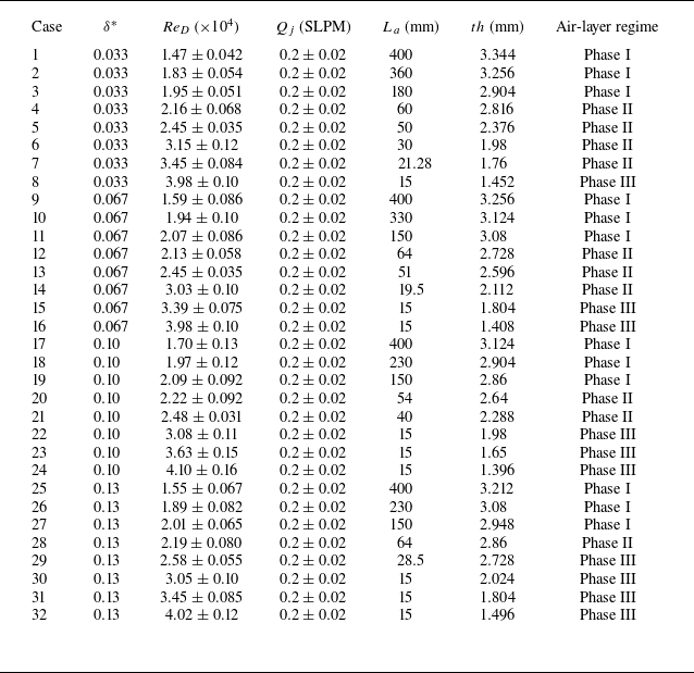

 x∗
 y∗
 th

 η
 th
 δ∗≈0.067,ReD≈2.07×10⁴
 δ∗≈0.13,ReD≈2.01×10⁴
 δ∗≈0.067,ReD≈2.13×10⁴
 Qj=0.2SLPM

 ReD≈(1.5±0.2)×104
 ReD≈(1.8±0.2)×104
 ReD≈(2±0.05)×104
 ReD≈(2.2±0.1)×104
 Qj=0.2SLPM
 λ
 δ

 300

 δBL
 x=Lg/2



