Introduction
Circularly polarized (CP) antennas are employed in many wireless communication systems due to their capabilities to suppress multi-path interference or fading, the ability to reduce the Faraday rotation effect due to the ionosphere, which can change the wave polarization by more than 360∘ [Reference Gao, Luo and Zhu1–Reference Richard and Henry3], and their potential to receive part of the available power from an impinging linearly polarized wave of arbitrary electric field orientation. In satellite communications, for example, a CP antenna is preferred to minimize possible losses caused by polarization mismatch between the incident wave and the receiving antenna. Due to these advantages, CP antennas are used in several applications, such as for space telemetry links. Notably, in the global positioning system (GPS), the requirements for an ordinary GPS antenna are generally (not limited to these): gain in the range of 3–5 dBic, bandwidth of 20.046 MHz in the L1 band and 20.46 MHz in both L2 and L5 bands, and right-hand circular polarization (RHCP). Further specifications may be phase-center stability, cross-polarization decoupling (XPD), and axial ratio (AR) [Reference Teunissen and Montenbruck4].
To enable a GPS antenna array to have an adaptive pattern, beam-forming techniques are essential. The choice of the magnitudes and the phases of the excitation coefficients needed to weight the signals received by the array elements make it possible to achieve beam steering while controlling the sidelobe level (SLL) simultaneously. For problems involving simple beam shapes and SLL control, pattern synthesis can be achieved using well-known techniques like the Fourier transform, Woodward–Lawson, and Dolph–Tschebyscheff. However, these methods typically do not consider mutual coupling and are normally applicable to arrays of isotropic antennas. Due to the complexity to calculate the magnitudes and phases of the excitation coefficients for each array element using analytical methods, global optimization techniques have been introduced. In the open literature, many articles report on the development of heuristic methods for array synthesis, such as the genetic algorithm (GA) [Reference Johnson and Rahmat-samii5], the particle swarm optimization [Reference Schlosser, Tolfo and Heckler6–Reference Abdulqader11], the firefly algorithm [Reference Yoshimoto and Heckler12, Reference Ram, Mandal, Kar and Ghoshal13], the ant colony optimization [Reference Quevedo-Teruel and Rajo-Iglesias14], and the cat swarm optimization [Reference Pappula and Ghosh15] to cite only a few. Some authors combine two optimization techniques to achieve the desired beam shape. Such approach is normally based on the combination of global and local optimization algorithms. In [Reference Ludwig-Barbosa, Schlosser, Machado, Ferreira, Müller Tolfo and Heckler16, Reference Schlosser, Heckler, Machado and Salazar17], the GA and the sequential quadratic programming were used to realize beamshaping and SLL control for linear antenna arrays.
Another heuristic applicable to pattern synthesis is the differential evolution (DE) method, introduced in 1996 by Rainer Storn and Kenneth Price [Reference Storn and Price18]. Due to its effectiveness and robustness for multi-variable optimization, the DE has been used to solve problems in many scientific and engineering fields, such as acoustics, aerodynamics, aeronautics, aerospace, automotive industry, and economics [Reference Qing19]. Many papers report on the use of DE to optimize antennas and antenna arrays. In [Reference Guney and Karaboga20], the DE technique has been applied to optimize the dimensionsof the aperture of a pyramidal horn aiming at gain enhancement. In [Reference Akdagli21–Reference Akdagli23], the synthesis and optimization of microstrip antennas using DE were proposed. The optimization of planar arrays with SLL control using DE was proposed in [Reference Rocha-Alicano, Covarrubias-Rosales, Brizuela-Rodriguez and Panduro-Mendoza24], whereby the array was composed of isotropic antennas and the mutual coupling between the array elements was neglected. In [Reference Yang and Nie25], the DE method was used to compensate for the mutual coupling effect in a linear antenna array. In [Reference Liu, Bai, Zheng, Liao, Ren and Guo26], a combined approach based on DE and the fast Fourier transform via the least-square active element pattern expansion has been applied for beam shaping with SLL control and side-band level of time-modulated antenna arrays. In [Reference Chen, Yang and Nie27], a modified DE strategy (MDES) is applied to synthesize patterns of linear antenna arrays, composed of isotropic elements, with configurations tailored to specific synthesis problems, such as monopulse arrays for sum and difference patterns and unequally spaced arrays. The analysis neglects mutual coupling between array elements, simplifying the design and focusing on pattern synthesis. The MDES, a refined version of the conventional DE, addresses challenges like premature convergence and slow optimization when solving complex, non-convex problems, such as antenna array synthesis. In [Reference Rocca, Oliveri and Massa28], the application of DE optimization strategies to electromagnetics theory is reviewed. Various DE strategies for antenna array pattern synthesis are discussed, focusing on metrics like SLL, beamwidth, directivity, and nulling. The conventional DE (DE/best/1/bin) strategy is highlighted as the most common and widely used approach for minimizing SLL in antenna arrays due to its robustness and efficiency to SLL minimization while maintaining manageable computational complexity. In [Reference Deb, Roy and Gupta29], the study examines different DE algorithms for antenna and antenna array design optimization, comparing DE variants like DEGL, SADE, MDE, and IDE. It benchmarks their performance across four cases: a 2.4 GHz probe-fed microstrip antenna, a cross-aperture-coupled microstrip antenna, an unequally spaced linear array, and a four-element Yagi–Uda antenna array.
An earlier version of this paper was presented at the 18th Conference of Antennas and Propagation (EuCAP 2024) and was published in its Proceedings [Reference Paulena, Vieira, Schlosser and Heckler30]. In this extended version, the conventional DE (DE/best/1/bin) method is applied to enhance beam steering, suppress SLL, and improve XPD. The DE/best/1/bin strategy is particularly well suited for these tasks due to its proven ability to provide robust solutions with manageable computational complexity [Reference Rocca, Oliveri and Massa28]. Notably, the optimization process incorporates mutual coupling and substrate truncation effects, unlike the works described in [Reference Rocha-Alicano, Covarrubias-Rosales, Brizuela-Rodriguez and Panduro-Mendoza24, Reference Chen, Yang and Nie27, Reference Deb, Roy and Gupta29], which assume isotropic array elements and neglected these critical factors. A key innovation in this work is the introduction of an additional pattern specification (mask) for cross-polarization suppression, which effectively enhances the AR while maintaining beam-steering capabilities. The effectiveness of the proposed approach is demonstrated with two different arrays: the first is composed of linearly polarized (LP) rectangular microstrip patches with sequential rotation; and the second comprises microstrip corners-truncated RHCP patches without sequential rotation. The main optimization goals are SLL control and enhancement of XPD while performing precise beam steering. The results obtained are compared to those achieved using the classical progressive phase shift (PP) technique and Dolph–Tschebyscheff distribution.
The paper is organized as follows: the DE algorithm is described briefly in Mathematical background for the Differential Evolution Method. In Optimization of 4×4 planar antenna arrays, the method is applied for the synthesis of planar antenna arrays with beam steering along with cross-polarization suppression. Numerical results are presented in Results. Finally, the conclusions are drawn in Conclusions.
Mathematical background for the DE method
The DE method, proposed by R. Storn and K. Price in 1996, is a stochastic global optimization heuristic, which emerged from attempts to solve a Chebychev polynomial curve fitting problem [Reference Price, Storn and Lampinen31]. This method aims at solving problems through consecutive iterations and differences between vectors, looking for possible solutions in individuals that compose a population. Basically, the method is divided into three steps: mutation, crossover, and selection. In the next subsections, each of these steps are described in detail.
Mutation
Initially, the method creates an initial population of NP parameter vectors  $\textbf{{x}}_{i}^{(G)}$, where G is the generation number and
 $i=1,2,...,N_P$ denotes each ith individual in the population. Each element of
 $\textbf{x}_{i}^{(G)}$ is chosen randomly with uniform distribution, resulting in a matrix with dimension
 $[N_P\times D]$, with D being the number of genes that compose an individual. The mutation process consists of adding a perturbation into the individual
 $\textbf{x}_{r_1}^{(G)}$ by means of the difference between two other individuals
 $\textbf{x}_{r_2}^{(G)}$ and
 $\textbf{x}_{r_3}^{(G)}$. This procedure aims at generating a mutant population and is executed mathematically by
 \begin{equation}
\textbf{m}_{i}^{(G+1)} = \mathbf{x}_{r_1}^{(G)} + F\left(\textbf{x}_{r_2}^{(G)} -\textbf{x}_{r_3}^{(G)}\right),
\end{equation}
where r 1, r 2, and r 3 are individuals selected randomly from the Gth population. For meaningful results, it is mandatory that  $r_1 \neq r_2 \neq r_3$. Therefore, in order to carry out the mutation step, NP must be larger than three and should not be changed throughout the optimization process. The factor F is a real and scalar constant that controls the intensity of the mutation and can be chosen in the range
 $[0,\:2]$ [Reference Storn and Price18]. At the end of the mutation process, each individual from
 $\textbf{m}_{i}^{(G+1)}$ has dimension
 $[1\times D]$.
Crossover
In order to increase diversity between the populations, crossover is included in the algorithm. This process consists of combining genes of two randomly chosen individuals from the Gth population, in order to yield a new generation. The selection criterion is based on a crossover probability Cr that can be set in the range [0,1]. The cross population is formed by
 \begin{equation}
c_{ij}^{(G+1)} = \left \{\begin{matrix} {m}_{ij}^{(G+1)}, & {if}\:\: \operatorname{rand}(j) \lt C_r\:\: {or}\:\: j=k(i) \\ {x}_{ij}^{(G)}, & {if}\:\: \operatorname{rand}(j) \ge C_r\:\: {and}\:\: j\ne k(i) \end{matrix} \right.,
\end{equation}
where  $j = 1,2,...,D$,
 $\operatorname{rand}(j)$ denotes the jth evaluation of a uniformly distributed random value within range
 $[0, 1]$ and k(i) is a randomly selected integer in the range
 $[1, D]$. This last term is inserted in the expression, in order to guarantee that at least one gene from
 $\mathbf{m}_{i}^{(G+1)}$ passes to
 $\textbf{c}_{i}^{(G+1)}$. This crossover method, as originally presented by Storn and Price, is called binomial crossover [Reference Storn and Price18].
Selection
In this step, the initial population  $\textbf{x}_{i}^{(G)}$ is compared to the cross population
 $\textbf{c}_{i}^{(G+1)}$. The greedy criterion is used to perform the selection of individuals that will compose the new population
 $\textbf{x}_{i}^{(G+1)}$. Mathematically,
 \begin{equation}
\textbf{x}_{i}^{(G+1)} = \left \{\begin{matrix} \textbf{x}_{i}^{(G)}, & {if}\:\: f\left(\textbf{c}_{i}^{(G+1)}\right) \geq f\left(\textbf{x}_{i}^{(G)}\right) \\ \textbf{c}_{i}^{(G+1)}, & {if}\:\: f\left(\textbf{c}_{i}^{(G+1)}\right) \lt f\left(\textbf{x}_{i}^{(G)}\right) \end{matrix} \right.,
\end{equation}
where  $f\left(\textbf{c}_{i}^{G+1}\right)$ and
 $f\left(\textbf{x}_{i}^{(G)}\right)$ are the values of the fitness function of each individual, which is related to the individual ability to solve the problem, i.e., in the case of a minimization problem, the lower the individual fitness is, the closer it is to the optimum solution.
Optimization of 4×4 planar antenna arrays
In this section, the DE method is applied to synthesize the radiation pattern of two  $4\times4$ CP microstrip antenna arrays designed to operate at 1.575 GHz (L1 band). The first array, depicted in Figure 1(a), consists of 16 LP rectangular microstrip patches, which are sequentially rotated to allow achieving CP. The main drawback of this array configuration is the generation of significant levels of cross-polarization, if beam steering in directions off the boresight are desired [Reference Gao, Luo and Zhu1]. The second array, shown in Figure 1(b), is composed of 16 singly-fed corners-truncated RHCP microstrip patches. Since the array elements are already CP, no sequential rotation is needed and lower SLLs in the cross-polarization are normally achieved. For both arrays, the aperture is located in the xy-plane; the elements are spaced by 0.5λ 0, whereby λ 0 is the wavelength in free space.
 $4\times4$ Microstrip antenna arrays considered: (a) array with linearly polarized (LP) elements; (b) array with RHCP elements.

The mathematical representation of the total electric field  $(\vec{E}_T)$ radiated by a planar array is given by
 \begin{equation}
\vec{E}_i^{(G)}(\theta,\phi)=\vec{E}_T \left(\theta,\phi,\mathbf{x}_i^{(G)}\right) = \sum_{j=1}^{D} x_{ij}^{(G)}\vec{E}_j(\theta, \phi),
\end{equation}
where D corresponds to the total number of elements that compose the array (in the present cases, D = 16),  $\mathbf{x}_{i}^{(G)}$ corresponds to
 $[I_1\angle{\delta_1} \:I_2\angle{\delta_2}\cdots I_D\angle{\delta_D}]$ where ID and δD are, respectively, the magnitude and the phase of the excitation coefficient that should weight the electric field radiated by the jth antenna, so as to yield the desired radiation pattern. It is important to mention that
 $\vec{E}_j (\theta,\phi)$ in (4) corresponds to the radiated electric field by the jth array radiator in the presence of the other elements (also called embedded element pattern), which must be calculated and extracted with a full-wave simulator. This procedure can be done by exciting the jth element with an incident voltage wave with magnitude equal to 1 V while terminating all others with matched loads. By doing so, the mutual coupling as well as GND and substrate truncation effects are taken into account in the entire optimization process [Reference Pozar32]. In this work, this procedure has been carried out using the electromagnetic simulator ANSYS HFSS for both arrays.
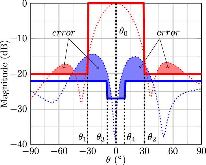
A typical mask used for antenna array synthesis defines the main-lobe region and sets the upper limit for the sidelobes. Such a mask is represented by the continuous red line shown in Figure 2. It specifies the main beamwidth, defined between the angles θ 1 and θ 2, and the beam-steering direction  $(\theta_0,\phi_0)$, where θ 0 represents the main beam direction in the elevation plane and ϕ 0 corresponds the main azimuth plane. The remaining angular regions state the maximum allowed SLL.
Definition of independent masks for co- and cross-polarizations: the mask for the co-polarization is defined by the solid red curve; the mask for the cross-polarization is defined by the solid blue curve.

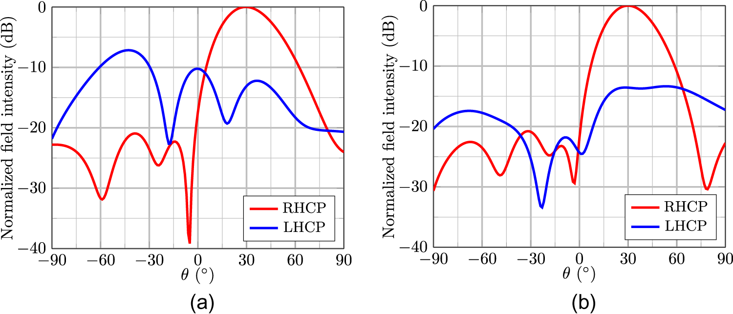
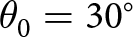
Generally, the optimization is done solely for the co-polarization pattern [Reference Schlosser, Tolfo and Heckler6, Reference Farias, Lemes, Vieira, Heckler and Salazar7, Reference Abdulqader11–Reference Ram, Mandal, Kar and Ghoshal13]. The consequence of that can be verified in Figure 3, which presents synthesized patterns for both arrays with beam steering to  $\left( \theta_0 ,\phi_0\right) = \left( 30^\circ ,0^\circ \right)$ and SLL of 20 dB for both antenna arrays depicted in Figure 1. In Figure 3(a), the optimized pattern of the antenna array composed of LP elements is presented, where the cross-polar component gain is relatively high: for
 $\theta = -47^\circ$, the cross-polar component gain is only 8 dB below the main beam level. Moreover, for both arrays, the XPD, defined as the difference between the co-polar and cross-polar component gains, is lower than 15 dB in the main lobe region. This corresponds to an AR greater than 3 dB, which is considered too high for applications requiring CP antennas.
Pattern optimization without considering the cross-polarization mask: (a) array with LP elements; (b) array with RHCP elements.

Since many modern communication systems demand precise polarization control to optimize their performance, large isolation between co- and cross-polarizations is crucial to ensure high polarization purity. To mitigate polarization degradation during the optimization process, a second mask to manage the cross-polar component gain can be employed, as indicated by the blue line in Figure 2. Specifically, the maximum allowable cross-polar component gain in the main lobe region is defined between the angles θ 3 and θ 4 to enhance the XPD, resulting in improved polarization purity, reduced AR and also a broader AR beamwidth.
With the red and blue masks defined in Figure 2, the purpose of the optimization process is to minimize the individual’s fitness function ( $\operatorname{fit}$), which is used to compute the deviation of the synthesized pattern from the desired one (mask). Mathematically,
 \begin{align}
& {fit}_i^{(G)}=f\left(\mathbf{x}_i^{(G)}\right)\nonumber\\
& = \sum _{b=1}^{N_\theta} w \left(\left | \left| {E}_{RH,i}^{(G)}(\theta_b,\phi_0) \right|_{\text{dB}} -\left|E_{RH,\text{mask}}(\theta_b,\phi_0) \right |_{\text{dB}}\right| +\ldots\right. \nonumber\\
& \left. \ldots \left | \left| E_{LH,i}^{(G)}(\theta_b,\phi_0)\right|_{\text{dB}} -\left|E_{LH,\text{mask}}(\theta_b,\phi_0) \right |_{\text{dB}} \right|\right),
\end{align}
where θb is the discrete value of θ within the range  $-90^\circ \le \theta \le 90^\circ$, thus
 $N_\theta=180$ and ϕ 0 is the steering plane. The subscripts RH and LH denote the right- and left-hand polarizations, respectively, of the synthesized electric fields and the radiation masks. For the correct application of (5), the fields
 ${E}_{RH,i}^{(G)}$ and
 ${E}_{LH,i}^{(G)}$, which are complex values, must be expressed in decibels. In contrast, the variables
 $E_{RH,\text{mask}}$ and
 $E_{LH,\text{mask}}$, representing the amplitude bounds for the desired radiation pattern, are purely real values provided in decibels. The parameter w can be set to weight the error obtained when the maximum direction of the synthesized patterns is different from the desired, i.e.,
 $E_{RH,i}^{(G)}(\theta_{0},\phi_0)~\neq~0$ dB,
 $w=2\times10^3$; on the other hand, when
 $\theta_{b}\neq\theta_{0}$,
 $w~=~1$. This ensures that the main beam will be steered precisely to the desired direction
 $(\theta_0,\phi_0)$. The fields
 ${E}_{RH,i}^{(G)}$ and
 ${E}_{LH,i}^{(G)}$ are calculated applying (4) with the following modifications
 \begin{equation}
{E}_{RH,i}^{(G)}(\theta,\phi) = {E}_{RH,T}^{(G)}\left(\theta,\phi,\mathbf{x}_{i}^{(G)}\right)= \sum_{j=1}^{D} x_{ij}^{(G)}{E}_{RH,j}(\theta, \phi),
\end{equation}
 \begin{equation}
{E}_{LH,i}^{(G)}(\theta,\phi) = {E}_{LH,T}^{(G)}\left(\theta,\phi,\mathbf{x}_{i}^{(G)}\right)= \sum_{j=1}^{D} x_{ij}^{(G)}{E}_{LH,j}(\theta, \phi),
\end{equation}
where  ${E}_{RH,j}(\theta,\phi)$ and
 ${E}_{LH,j}(\theta,\phi)$ correspond, respectively, to the RHCP and LHCP active field (embedded pattern) components extracted from HFSS.
For this work, the application of (5) will be based on the masks for RHCP and LHCP patterns defined, respectively, as
 \begin{equation}
\left|E_{RH,{mask}}(\theta,\phi)\right|_{{dB}} = \begin{cases}
-20~\text{dB}, & -90^\circ \lt \theta \lt \theta_1 \\
0~\text{dB}, & \theta_1 \lt \theta \lt \theta_2 \\
-20~\text{dB}, & \theta_2 \lt \theta \lt 90^\circ \\
\end{cases}
\end{equation}
 \begin{equation}
\left|E_{LH,{mask}}(\theta,\phi)\right|_{{dB}} = \begin{cases}
-20~\text{dB}, & -90^\circ \lt \theta \lt \theta_3 \\
-25~\text{dB}, & \theta_3 \lt \theta \lt \theta_4 \\
-20~\text{dB}, & \theta_4 \lt \theta \lt 90^\circ. \\
\end{cases}
\end{equation}
Results
In this section, the results obtained for both arrays illustrated in Figure 1(a) and (b) using the DE method along with the dual-mask approach are presented. The results are compared to those obtained using PP and Dolph–Tschebyscheff method with progressive phase shift (DTPP). In both cases, the radiation patterns are steered to four directions in the  $\phi_0=0^\circ$ and
 $\phi_0=45^\circ$ planes. The latter has been chosen, since it is the most challenging case for cross-polarization suppression.
For both arrays, the DE algorithm was configured with 100 individuals, maximum number of iterations equal to 3000,  $F~=~0.1$ and
 $C_r = 0.5$. Table 1 lists the mask parameters used for different beam-steering directions. The desired SLL was set to 20 dB below the main lobe for all cases and the cross-polar component gain was set to 25 dB between the angles θ 3 and θ 4, to ensure high CP purity.
Mask parameters used in the optimizations

Optimization of a 4×4 LP microstrip antenna array with sequential rotation
The simplest and well-known method to steer the main lobe of an antenna array is based on the application of PP between the elements. However, a drawback of this approach is that it can yield patterns with large SLL, because it does not optimize the amplitude distribution across the array aperture. In Figures 4 and 5, the results obtained using this scanning principle are shown by the dotted red lines. Deviations from the desired steering direction at large angles off from the boresight can be seen in the calculated patterns. For the steering directions  $\theta _0 = 20^\circ$ and
 $\theta _0 = 30^\circ$, a main lobe squint of 2∘ was observed. For
 $\theta _0 = 40^\circ$ and
 $\theta _0 = 50^\circ$, the respective deviations are 3∘ and 7∘. This occurs because each element in the array exhibits its unique embedded pattern. Moreover, it leads to increased SLLs, thereby reducing the efficiency and accuracy of the beam pointing [Reference Balanis33]. The use of DTPP has been also tested for SLL suppression and the results are shown in dash-dotted lines. The technique yields acceptable results for steering angles close to the boresight. However, for large scanning angles, the specifications for both SLL and XPD are not fulfilled.
Comparison between the optimized radiation patterns in the  $\phi_0=0^\circ$ plane for the
 $4\times4$ planar array composed of LP patches with PP (dotted lines), DTPP (dash-dotted lines), and DE (solid lines): (a)
 $\theta _0 = 20^\circ$; (b)
 $\theta _0 = 30^\circ$; (c)
 $\theta _0 = 40^\circ$; (d)
 $\theta _0 = 50^\circ$.

Comparison between the optimized radiation patterns in the  $\phi_0=45^\circ$ plane for the
 $4\times4$ planar array composed of LP patches with PP (dotted lines), DTPP (dash-dotted lines), and DE (solid lines): (a)
 $\theta _0 = 20^\circ$; (b)
 $\theta _0 = 30^\circ$; (c)
 $\theta _0 = 40^\circ$; (d)
 $\theta _0 = 50^\circ$.

The DE method was applied to minimize the main lobe squint, control the SLL, and minimize cross-polarization levels, especially in the main beam region. The results indicated by the continuous lines in Figure 4 show that the optimization process successfully yields patterns with the main beam steered to the desired directions in three cases. For  $\theta_0=50^\circ$, a deviation of only 1∘ was observed. Furthermore, the optimized patterns respected the boundaries imposed by the masks for both polarizations, XPD values greater than 25 dB in the main beam direction were achieved in all cases. The SLL was controlled at 20 dB below the main beam, as defined in (8)–(9) and Table 1. However, for
 $\theta_0=50^\circ$, the SLL was not effectively controlled at the edge directions, which can be attributed to the limitations imposed by the physics of the array factor. When comparing DTPP and DE, it is evident that optimizing both amplitude and phase enables effective beam steering over a wide range while keeping high XPD and controlled SLL simultaneously.
Figure 5 shows the radiation patterns for beam steering in the  $\phi_0 = 45^\circ$ plane, using the PP, DTPP, and DE. As the main beam is steered toward angles increasingly distant from the boresight, the cross-polarization level tends to rise significantly using PP and DTPP. This increase in cross-polarization leads to a degradation in polarization purity and can negatively impact the overall performance, especially in applications requiring high polarization purity. The results obtained with DE using the proposed dual-mask approach exhibit large XPD, ensuring high polarization purity, along with effective control of the sidelobes levels and cross-polarization component across the entire
 $\phi_0 = 45^\circ$ plane. These results ensure improved CP purity and higher overall array performance, even when the beam is steered far away from the boresight. The beam-forming coefficients obtained with DE to steer the main lobe toward
 $\theta_0=50^\circ$ and
 $\phi_0=45^\circ$, as listed in Table 2, yield the radiation pattern depicted by the continuous lines in Figure 5(d).
Normalized excitation coefficients optimized to point the main beam to  $\theta_0 = 50^\circ$ and
 $\phi_0 = 45^\circ$ with SLL
 $\leq-20$ dB

Optimization of a 4×4 RHCP microstrip antenna array
The second antenna array considered to demonstrate the proposed approach based on independent masks for co- and cross-polarizations is composed of RHCP patches without sequential rotation. As observed in Figure 6, the criteria for SLL and XPD are not fulfilled with DTPP, especially when the beam is steered away from the boresight. This outcome occurs because the Dolph–Tschebyscheff technique is based on the classical array theory, which considers only isotropic elements [Reference Balanis33]. Additionally, it fails because mutual coupling and the truncation of GND and substrate are present in realistic microstrip antenna arrays. This highlights the limitation of the Dolph–Tschebyscheff method for beam-steering applications.
Comparison between the optimized radiation patterns in the  $\phi_0=0^\circ$ plane for the
 $4\times4$ planar array composed of RHCP patches with DTPP (dash-dotted lines) and DE (solid lines): (a)
 $\theta _0 = 20^\circ$; (b)
 $\theta _0 = 30^\circ$; (c)
 $\theta _0 = 40^\circ$; (d)
 $\theta _0 = 50^\circ$.

The results obtained with DE are shown by the continuous lines in Figure 6. They demonstrate that effective control of the SLL and significant improvement in XPD could be achieved with the proposed technique.
Figure 7 compares the performance of the tested methods for beam steering in the  $\phi_0=45^\circ$ plane. As shown, there is a significant difference in cross-polarization performance: while the DTPP method resulted in a low SLL, it failed to maintain the XPD above the desired value. On the other hand, the DE algorithm achieved enhanced performance with XPD levels exceeding 25 dB. This improvement also led to a broader AR beamwidth in the
 $\phi_0=45^\circ$ plane, hence indicating better polarization purity across a wider angular range. The optimized excitation coefficients to steer the main lobe toward
 $\theta_0=50^\circ$ and
 $\phi_0=45^\circ$ are listed in Table 3. These coefficients produce the radiation pattern depicted by the continuous lines in Figure 7(d).
Comparison between the optimized radiation patterns in the  $\phi_0=45^\circ$ plane for the
 $4\times4$ planar array composed of RHCP patches with DTPP (dash-dotted lines) and DE (solid lines): (a)
 $\theta _0 = 20^\circ$; (b)
 $\theta _0 = 30^\circ$; (c)
 $\theta _0 = 40^\circ$; (d)
 $\theta _0 = 50^\circ$.

Normalized excitation coefficients optimized to point the main beam to  $\theta_0 = 50^\circ$ and
 $\phi_0 = 45^\circ$ with SLL
 $\leq-20$ dB

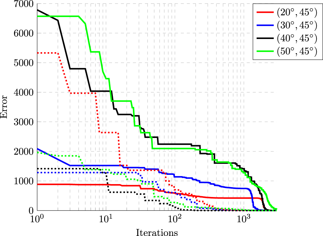
Table 4 summarizes the XPD levels and AR beamwidths obtained in the main beam directions using the PP, DTPP, and DE methods for each antenna array. The AR beamwidth is defined as the angular range where the AR remains below 3 dB. Figure 8 presents the evolution curves of the error function at each iteration for the steering cases in the  $\phi_0=45^\circ$ plane. Since the optimization method is based on a stochastic process, each curve has different initial and final values for the error function. Despite this variability, the method achieved favorable outcomes, hence demonstrating its robustness to minimize the error function.
Error evolution curves for beam-steering cases to  $\phi_0=45^\circ$ for array composed of LP elements (solid lines) and array composed of RHCP elements (dotted lines).

Comparison between XPD and AR beamwidth obtained at the main beam direction

* Cases that the axial ratio level in the main lobe region is greater than 3 dB.
Conclusions
This paper demonstrated the use of the DE method for optimizing two  $4\times 4$ planar antenna arrays, each composed of different types of microstrip patch antennas. The extension proposed in this paper was based on the use of independent pattern masks for co- and cross-polarizations.
The synthesized patterns obtained with the proposed approach exhibited superior performance in comparison to results yielded by two other classical excitation methods, particularly in terms of XPD in the steering direction, thereby enhancing the AR beamwidth. The optimization strategy has been tested successfully for four steering directions in two different planes ( $\phi_0=0^\circ$ and
 $\phi_0=45^\circ$).
It is evident that for the antenna array with LP elements, the XPD is significantly degraded when the beam is steered away from the boresight direction unless an optimization method is employed. For the antenna array with RHCP elements, the DTPP method achieves satisfactory results in terms of SLL control; however, as the main beam is steered away from the boresight, the XPD is not effectively managed. In contrast, the DE algorithm achieves consistent results for both antenna arrays, since it allowed steering the main beam effectively while maintaining SLL and XPD within the mask constraints and improving the AR beamwidth.
All the simulations presented could be done in less than 3 minutes running a MATLAB code on a PC with Intel(R) Core(TM) i3-5005U CPU @ 2.00 GHz processor and 8 GB RAM. Therefore, the use of DE allowed achieving excellent results with fast convergence and low computational cost.
Acknowledgements
This work has been partially supported by the Coordenação de Aperfeiçoamento de Pessoal de Nível Superior (CAPES) (Finance Code 001) and by the National Council for Scientific and Technological Development (CNPq) under grants 300060/2023-8, 305654/2022-5, 407245/2022-7, and 406517/2022-3 (INCT-Signals).
Competing interests
The authors declare none.

Juner M. Vieira was born in Alegrete, Brazil, in 1984. He received the B.Sc. degree in telecommunications engineering from the Universidade Federal do Pampa (Unipampa), Brazil, in 2017, the M.Sc. degree in electrical engineering from the same institution in 2019, and his Ph.D. in electronics engineering focusing on microwave and optoelectronics from the Aeronautics Institute of Technology (ITA), Brazil, in 2023. He is currently a Technological Development fellowships holder within the Space Electronics and Computing Division at National Institute for Space Research (INPE), Brazil. His research interests include microwave circuits, microstrip antennas, and antenna arrays.

Edson R. Schlosser was born in Santa Rosa, Brazil, in 1989. He received the B.Sc. and M.Sc. degrees in electrical engineering from Universidade Federal do Pampa, Brazil, in 2011 and 2014, respectively, and the Ph.D. degree from Pontifícia Universidade Católica do Rio de Janeiro, Brazil, in 2020. Since 2013, he is professor at Universidade Federal do Pampa, Alegrete, Brazil. His current research interests are the design of microstrip antennas, arrays and reflectarrays, synthesis of radiation patterns using meta-heuristics, and design of passive microwave devices based on lumped elements.

Gabriel P. Paulena was born in Mogi das Cruzes, Brazil, in 2000. He received the B.Sc. degree in telecommunications engineering from the Universidade Federal do Pampa (Unipampa) in 2023. He is currently an MS student in Electrical Engineering (Communication Systems) at the same institution. His main research interests are the design of dielectric resonator antenna and arrays for telemetry applications and the implementation of optimization heuristics for beamforming.

Marcos V. T. Heckler was born in Rio Grande, Brazil, in 1978. He received the B.Sc. degree in electrical engineering (emphasis in electronics) from the Universidade Federal de Santa Maria (UFSM), Brazil, in 2001, the M.Sc. degree in electronic engineering (microwaves and optoelectronics) from Instituto Tecnológico de Aeronáutica (ITA), Brazil, in 2003, and the Dr.-Ing. (Ph.D.) degree from the Technische Universität München, Munich, Germany, in 2010. From April to August 2003, he worked as a Research Assistant with the Antennas and Propagation Laboratory, ITA, Brazil. From October 2003 to June 2010, he worked as a Research Associate with the Antenna Group, Institute of Communications and Navigation, German Aerospace Center (DLR), Oberpfaffenhofen, Germany. Since 2010, he is professor at Universidade Federal do Pampa, Alegrete, Brazil. His current research interests are the design of microstrip antennas and arrays and the development of numerical techniques for microstrip antennas.