

1 Introduction
Inequality is an important factor in today’s globalization of the world economy and one of the underlying causes of income inequality — educational inequality — is at the core of the debate. Educational inequality is in many cases difficult to measure because micro surveys, which are not normally comparable across countries and periods, are necessary. This contribution uses the numeracy difference between occupational groups as a measure of inequality for the period from the 18th to the early 20th centuries, and the difference in years of schooling between the taller and shorter half of the female population as a measure for late 20th century educational inequality. For the earlier period we concentrate on Latin America, a region where 20th century income inequality is famously high, and for the latter period we compare the countries of this region with less developed countries (LDCs) and medium-income countries elsewhere.
The relationship between globalization and educational inequality is one of today’s major issues. Is it possible that the current globalization will fail, just as the previous globalization tendency in the period 1850-1914 did, because inequality stimulates anti-integration forces? Timmer and Williamson (Reference Timmer and Williamson1998) found that during the 19th century, inequality in new world countries such as the United States, Brazil, Argentina, Canada and Australia provoked anti-immigration policies that led to the disintegration of Atlantic labor markets. Rising inequality could also decrease the legitimation of international integration, so that those groups that normally benefit from it (e.g. the well educated in rich countries and world inhabitants in general) might not give it their full support.
There are other reasons why the study of educational inequality determinants is important. First, inequality is now often considered as a component of the standard of living. Being at the bottom of the income distribution is much harder to bear if the distance to the wealthier part of the economy is large, and educational inequality is a determinant of later income inequality. This also applies to the inequality of schooling (Castello and Domenech Reference Castello and Domenech2002; Thomas et al. Reference Thomas, Wang and Fan2001).
Wood (Reference Wood1997) argued that for the 1980s and 1990s more open trade increased wage inequality in some parts of the world, particularly in Latin America (Wood Reference Wood1997; UN 1995; Cepal 2004). His studies have focused on the 1980s and 1990s. The question is whether the relationship of globalization and inequality holds before the 1980s. In our study, we are not restricted to only two decades. We are able to analyze the relationship for three centuries and will assess the difference between educational inequality in the «First Era of Globalization Period», as O’Rourke and Williamson (Reference O’Rourke and Williamson1999) defined it — namely, the 1850-1913 period — with the early phases. For the second study period, 1945-1984, we will use the openness indices of Sachs and Warner (Reference Sachs and Warner1995) as well as trade shares to assess whether openness increased educational inequality. Inequality, though, is a complex phenomenon and many potential determinants should be taken into account as well as globalization. We will therefore control for as many other potential determinants as possible.
Why should openness matter for educational inequality? Most research in this field has focused on income inequality in OECD countries, arguing that imports of goods mainly produced with unskilled labor could decrease the demand for unskilled labor within the rich OECD countries, depressing unskilled wages and increasing inequality. However, factor endowments and relative scarcities in developing countries (LDCs) differ fundamentally (Wood Reference Wood1994, Reference Wood1997, Reference Wood1998).
Our expectation is that openness in fact increases inequality in countries with abundant land, and lowers inequality if unskilled labor, relative to potential trading partners, is the abundant factor. In the absence of unusual complementarities between factor inputs and other counteracting forces, poor countries will increase their exports of unskilled labor-intensive products during globalization periods because their abundant factors and their comparative advantage are likely to be in this segment. Increasing production with unskilled labor should increase unskilled labor demand and wages, and the opposite should be true for land-rich countries. If labor demand rises (falls), even children of unskilled workers should receive some schooling (or less), although in most cases not enough to move into the upper half of income recipients.
Now, Latin America was clearly a land-rich region between the 18th and early 20th centuries (Prados de la Escosura Reference Prados de la Escosura2007). Therefore, the expectation would be a rise in inequality during the «First Era of Globalization» (1850-1913; O’Rourke and Williamson Reference O’Rourke and Williamson1999). Does the expectation also hold for the broader sample of developing countries during the 1945-1984 period? It is somewhat less clear as some were already industrializing during the period and land became less important.
A number of scholars have studied the influence of globalization and de-globalization on within-country income inequality worldwide (Lindert and Williamson Reference Lindert and Williamson2001). Bourguignon and Morrison (2002) found a strong decline of within-country inequality during the de-globalization phase of 1914-1945, whereas within-country inequality rises during globalization phases. Prados de la Escosura (Reference Prados de la Escosura2007) finds increasing Latin American income inequality during this period. In section 5, we will assess whether educational inequality also increases with growing openness.
2 Years Of Schooling, Age Heaping, Occupations And Inequality
We will first discuss the general idea of the age-heaping method in this section, before discussing our measures for inequality of human capital. Age heaping is often used nowadays as a basic numeracy indicator. The share of people who are able to report their exact age rather than a rounded age has been found to be strongly correlated with numerical abilities (Crayen and Baten Reference Crayen and Baten2010a). A widely used measure for age heaping is the ABCC index, as suggested by A’Hearn et al. (2009), which divides the number of people who reported non-preferred ages (i.e. ages that are not a multiple of five) by the total number of peopleFootnote 1. The index ranges from 0 to 100. If everybody reports the correct age, ABCC has a value of 100. Here, we restrict the evidence to the age groups 23-32, 33-42, 43-52 and 53-62 years, because ABCCs of younger and older individuals might be biased. Only units that have at least thirty cases per skill and age group are studied. The ABCC index can best be understood by considering an example. If we have 100 people with unskilled occupations of a specific age group reporting age in the census of, say, 1870, we would expect twenty of them to report an age ending in zero or five (because two of ten ages end in zero or five). For the remaining eighty individuals, the question is: do they report other ages or do they also choose an age ending in zero or five? If twenty do the latter, then one-quarter (of the eighty remaining persons) report probably a wrong age, and the ABCC is then 75 per cent (one minus one-quarter). If the people with skilled occupations in the same country and birth decade have an ABCC of 85 per cent, then the social difference of numeracy between those occupational groups is ten (85-75 per cent)Footnote 2.
It is important, however, to countercheck whether the census-takers or recruitment officers did explicitly ask for the age (and did not «correct» the reported ages afterward). In the case of the samples studied here, we have good reasons to believe that the people were actually asked for their age, and the number of corrections made afterward was not large. Otherwise, the relatively high level of age heaping that we observed in the data would probably not have occurredFootnote 3.
How close is the relationship between age heaping and other human capital indicators such as literacy and schooling? A’Hearn et al. (Reference A’Hearn, Crayen and Baten2009) used the large US census sample to perform a very detailed analysis of this relationship. They subdivided by race, gender, high and low educational status and other criteria. In each case, they obtained a statistically significant relationship. The fact that the coefficients are relatively stable between samples is also noteworthy, that is, a unit change in age heaping is associated with similar changes in literacy across the various tests. The correlation was both statistically and economically significant for any country studied so far that had substantial age heapingFootnote 4.
Some uncertainty remains about whether age heaping in the sources contains information about the numeracy of the responding individual or, rather, about the diligence of the reporting personnel who wrote down the statements. A potential bias always exists if more than one person is involved in the creation of a historical source. For example, if literacy is measured by analyzing the share of signatures in marriage contracts, there might have been priests who were more or less interested in obtaining real signatures, as opposed to just crosses or other symbols. We find it reinforcing that we estimate generally much more age heaping (and less numeracy) for the lower social strata, and among the half of the sample population that had lower anthropometric values. Moreover, the regional differences of age heaping are similar to regional differences in illiteracy.
We conclude that the age-heaping method is now a well-established indicator for numeracy of groups, but the problem regarding how upper and lower group members can be distinguished from each other for historical populations for which we typically have no individual income data remains. Occupations have often been used to classify upper- vs. lower-income group individuals and we will apply this criterion to Latin American data until the 20th century (similarly to Crayen and Baten Reference Crayen and Baten2010b). Of course, occupations such as «day laborer» or «agricultural worker» typically yielded a low income, whereas professionals, noblemen, factory owners and skilled craftsmen had higher incomes. As a caveat to this method, it should be noted that some occupations represent a wide income range (e.g. farmers).
For the study of the 1945-1984 period, we also use an alternative, similarly rough proxy to distinguish between social groups, based on human stature as Crayen and Baten (Reference Crayen and Baten2010b) have suggested. This involves contrasting the number of years of schooling of the taller and shorter 50 per cent of the sample. Almost all anthropometric studies that considered occupational or income groupings found that the well-off strata of society were tallerFootnote 5. A second, very interesting aspect of this strategy is that tall individuals are much less likely than short individuals to have suffered from infant protein deficiency syndrome, which reduces learning abilities to a certain extent. The syndrome was widespread during the 1945-1984 period in the poorest countries of the world, when malnutrition was so common that most populations were severely stunted (with adult males being shorter than 170 cm on average). Support for this claim comes from biologists and psychologists who have conducted experiments on the influence of protein malnutrition in childhood and intellectual ability later in life (Paxson and Schady Reference Paxson and Schady2007).
One caveat to the proposed anthropometric method is clearly that there is also genetic height variation (especially on the individual level, see Magnusson et al. Reference Magnusson, Rasmussen and Gyllenstein2006). Nonetheless, we are confident that most individual variation can be averaged out by means of sufficiently large sample sizes.
Why do we use such a special method to measure inequality of education? Are there not other data sets available that contain some social classification criterion (such as occupation or income), as well as educational measures for the 1945-1985 period? To the best of our knowledge, for such a large number of countries as used here (forty-two countries), consistent data sets of this type do not existFootnote 6.
3 Data Sources, Selectivities And Representativeness
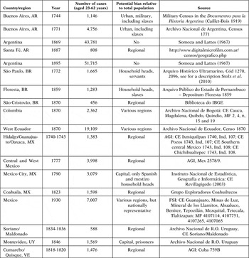
Many population counts were carried out in colonial Latin America, aiming at an overview of the population, taxpayers and the military potential. Most early counts were focused on limited regions or cities within a country. Larger censuses were carried out after the mid-18th century, covering a higher share of the national population (Table 1; Manzel and Baten Reference Manzel and Baten2010). For the post-colonial period, censuses of the republics were carried out mostly after the mid-19th century, while the early 19th century is clearly less documented. The Latin American countries currently have the best source situation of historical population enumerations among today’s developing countries (Platt Reference Platt1998, p. 7). Our samples cover Argentina, Brazil, Colombia, Ecuador, Mexico, Uruguay and VenezuelaFootnote 7 and therefore represent a large part of this world region. All in all, the countries under study today represent around 80 per cent of the Latin American population. An important question is whether our various sources are representative of the whole society during the period under study. This issue has been studied intensively by Manzel and Baten (Reference Manzel and Baten2010) who used mostly the same sources to study long-term trends. The population enumerations were supposed to have universal coverage in the whole area considered as well as in all social strata. Manzel and Baten have assessed many potential weaknesses of the data, such as social and regional biases. For example, one potential criticism of the padrones of the 18th century is under-enumeration. The government wanted to know the population number and age structure in order to learn about the potential of taxpayers. One could imagine that this stimulated avoidance behavior among the richer part of the population. However, it was not easy for the rich and well-educated strata to avoid being included in the census. We find them in large numbers in our census lists, as is evident from the occupations listed.
Another potential caveat is the problem regarding who really answered the question about age. Is it possible that perhaps only the head of the household answered for the whole house? Manzel and Baten (Reference Manzel and Baten2010) applied an indirect method by calculating the age-heaping indices for household heads and other members of the household. The expectation was that the head knew his exact age more often than the age of other household members. The difference between the two groups, however, was not very large. Other scattered evidence comes from remarks of the census officials about heads and other household members. In both cases, there were statements such as «she did not know her age», combined with an age statement of a preferred age. This can be interpreted as evidence that other household members were also actually questioned.
Ethnic composition is important for Latin America. Were Indios or slaves of African origin sometimes omitted from the padrones? The direct comparison of population structure by ethnic group given in the literature and the composition of 18th century padronesFootnote 8 revealed that the bias was limited Manzel and Baten (Reference Manzel and Baten2010; Table 3). In some Mexican censuses, there was some under-representation of American Indios and in one of the Buenos Aires padrones there was some under-representation of African Americans, but in general the samples were quite representative in terms of ethnicity.
Regional bias is another issue that we need to address. Clearly, the early samples in particular were more often concentrated on the population of the capital (Tables 1 and 2). Large cities tend to have higher levels of inequality (Baten Reference Baten1999), and hence we expect higher inequality values for the 18th century. We will assess this effect with appropriate dummy variables below.
DATA SOURCES FOR THE EARLY PERIOD

AGI: Archivo General de Indias, AR: Argentina, BR: Brazil, CE: census of; FSI: family search indexing project, MF: microfilm; MX: Mexico, UY: Uruguay, VE: Venezuela.
Sources: adapted from Manzel and Baten (Reference Manzel and Baten2010), plus other sources as explained in column «Source».
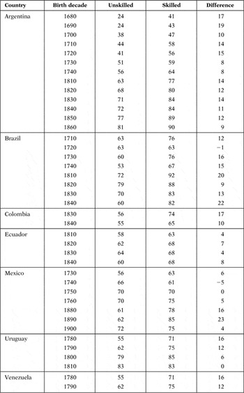
ABCC INDICES IN SEVERAL LATIN AMERICAN COUNTRIES BY BIRTH DECADE AND OCCUPATIONAL GROUPS

Notes: «Skilled» refers to occupational groups that were skilled, or professionals. «Unskilled» refers to those with unskilled or only semi-skilled occupations.
Finally, an important point for Latin America in particular is whether migrants should be included in the individual samples. Here, we are mainly interested in the educational inequality of countries and migrants who contributed to this inequality. Therefore, we decided to include migrants as wellFootnote 9.
While the sources for the study of Latin American educational inequality during the 18th to early 20th centuries deserve the most scrutiny, the later 20th century evidence, which we are employing for our second study period, is easier to use. The Macro International Inc. performs surveys of child health and health-related behavior in order to create a solid and representative database for improving child health (among other aims). They recorded years of schooling and heights of women mostly born between 1945 and 1984 in many developing countries. We included only those aged 20-50 years in many developing countries. As the height of adults is mostly determined in the 3 years after birth, the height of the mother can shed light on the development of status differences in this period after birth. One potential lacuna in our data is the environmental influence on growth at later ages, especially during the adolescent growth spurt. However, Baten (2000) finds that this effect is negligible compared to the impact of the first 3 years, as long as individuals have reached their final height when measured. Second, there could be survivor bias effects, but Moradi and Baten (Reference Moradi and Baten2005) and Guntupalli and Baten (Reference Guntupalli and Baten2006) rejected this possibility in detailed studiesFootnote 10.
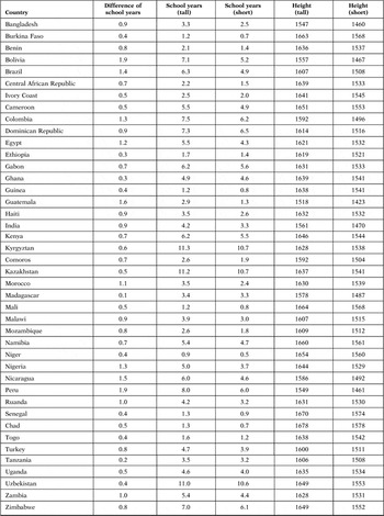
We consider here the difference in years of schooling of the taller 50 per cent compared with the shorter half, and organize the data by individual country and birth decade. It is remarkable that in most cases taller women had more years of schooling (Table 3). Small differences refer to cases such as Ghana, Madagascar or Tanzania, in which the urban centers of education differed from the regions of tallest heights, which were sometimes characterized by specialization in cattle farming (Moradi and Baten Reference Moradi and Baten2005). In Latin America, some of the strong educational inequalities by height group are partly determined by the Indio vs. European ancestor difference. It is difficult to disentangle socio-economic differences from nutritional habit differences (and perhaps genetic ones) here. Hence, we will rely on fixed effect regressions below, which control for country-specific characteristics.
DIFFERENCES OF SCHOOL YEARS BY HEIGHT (BIRTH YEARS 1945-1984)

Notes: «Tall» is defined here as the tallest 50%; «short» as the shortest 50%. The difference in school years is the number of school years of the taller minus the shorter 50%. Female height is reported in millimetres.
4 Development Of Educational Inequality
We would expect levels of educational inequality in the various countries of Latin America to be quite different because the institutional and economic structures were so varied. For example, Mesoamerica and the Andes had large shares of indigenous or mestizo populations, who received less schooling and other public goods compared with the middle and upper strata of European origin. In these regions, the inequality heritage of land distribution in favor of the Spanish conquerors and later European immigrants might have been strongest (Lambert Reference Lambert1968, p. 581)) Similarly, strong differences might have prevailed in the countries that kept slavery until the late 19th century and whose population component of African origin was disadvantaged. In contrast, the population of the Southern Cone was more homogeneous in ethnicity-related aspects, because the Indio population share was smaller and slavery was abolished earlier. However, ethnicity, slavery and colonial heritage were not the only factors at work. O’Rourke and Williamson (Reference O’Rourke and Williamson1999) argued convincingly that the Southern Cone countries had strongly increasing inequality during the late 19th century globalization movement.
Going further back in time, how might inequality have differed between colonial times and post-independence Latin America? Unfortunately, today we have little evidence for the pre-independence inequality history of Latin America. Williamson (Reference Williamson2009) and Dobado and Garcia (Reference Dobado and Garcia2009) have recently raised some doubts about the early colonial heritage hypothesis (of continuously high inequality). Dobado and Garcia argued that real wages were quite high in some parts of Bourbon Latin America, whereas average income was lower than in Europe. Hence, inequality might actually have been lower than in Europe. The question is, of course, whether this wage evidence is representative and can inform us about the situation of other poorer strata, which did not earn wages (such as the population majority of peasants). Williamson (Reference Williamson2009) considered the fact that especially the low population density of the 17th and early 18th centuries might have generated relatively low inequality, compared with Europe. In times of labor scarcity, wages tend to be higher and even the nutrition and general treatment of slaves and indigenous bound labor might be slightly less terrible. Recent study on Uruguay suggests that in the Southern Cone during the 18th century, inequality might also not have been very pronounced (Vicario Reference Vicario2010).
Economic policy differences certainly also mattered for country-specific differences. For example, the famous Mexican dictatorship era of Porfirio Díaz (1877-1911) increased average income and education, but had a reputation for bringing about sharp increases in inequality (Tutino Reference Tutino2001, pp. 700-701). In sum, during the 19th century the variation of inequality between countries was probably large. Pre-independence inequality history is largely unexplored, but some authors have recently argued for a modest inequality level relative to Europe.
In the following, we first compare numeracy of the upper and lower occupational strata in Latin American countries for the early period. For Argentina, we have some data for Buenos Aires for the birth decades until 1740 and some representative national data after this date. The ABCC index increased from 24 to 56 for the lower-income groups in Buenos Aires from the late 17th to the mid-18th centuries (Table 2). The upper-income groups started with a level above 40 per cent age numeracy in the 1680s, but grew to just 64 per cent in the 1740s. The fact that the early evidence on Argentina covers only Buenos Aires is certainly a caveat. The gap for the 19th century was large and relatively constant, declining only slightly from a 14 per cent difference in the 1820s to a 9 per cent difference in the 1860s.
Second, we have long-term data on Mexico covering sufficient observations to study both social groups between the 1730s and 1760s, and between the 1880s and 1900s. The latter evidence is nationally representative, while the former relates to some Mexican regions, including Mexico City. In short, social differences in age numeracy were small and in one case even negative in 18th century Mexico. This is consistent with the observation of Tanck de Estrada (Reference Tanck de Estrada1999) that the Bourbon reforms of the 18th century had some positive impact even on school building in Indio villages, that is, for the poorest Mexicans. However, the late 19th century saw a highly stratified society with large differences. This fits with available evidence on the Porfiriato.
We have more scattered data for a number of other Latin American countries (Table 2). In Brazil, the highest educational inequality levels were reached in the 1840s, which are the latest values we haveFootnote 11. In Uruguay, inequality was declining, but this might have been caused by the fact that the later birth cohorts were based on data from prisons. Venezuela and Colombia had quite high inequality, whereas in poor Ecuador even the skilled groups had low levels of numeracy. Summing up, we can document a number of Latin American countries, but the cases for which we have sufficient numbers of observations are somewhat distributed over the different centuries. Most striking in Table 2 is the fact that, of the forty cases studied, only two have negative values for the difference between the skilled and unskilled groups.
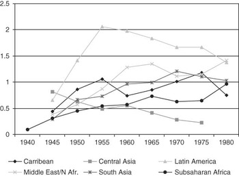
Now we move to the birth cohorts of the mid-to-late 20th century. We studied the difference of school years, subtracting the figure for the taller half from that of the shorter half (Figure 1). The years of schooling are a better measure for the mid-to-late 20th century than age heaping, which had already disappeared in many countries by then. It should be noted that there are many African countries in the sample, a few Latin American ones, but fewer countries from other regions. One important result from these samples is that the taller half of the population (those who probably came from more advantaged family backgrounds) always had higher or equal school year values, which tended to be lower among the shorter half of the populationFootnote 12. Latin America had the highest difference (which means the largest educational inequality), whereas Soviet Central Asia had the lowest value (Figure 1).
SCHOOL-YEAR DIFFERENCE (VERTICAL AXIS) IN SEVERAL WORLD REGIONS BY BIRTH YEARS
Notes: Difference in years of schooling, value of tallest 50 per cent minus the shortest 50 per cent (women). Years refer to the beginning year of a 5-year birth cohort. Central Asia includes only the former Soviet Republics.

5 Openness And Other Potential Determinants Of Inequality
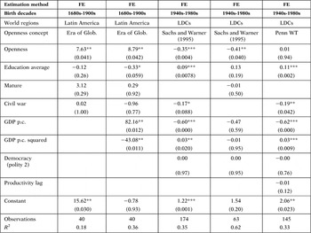
We first describe the explanatory variables in Table 4 that we include in the regressions and then discuss the results.
DETERMINANTS OF EDUCATIONAL INEQUALITY

FE: fixed effects, LDCs: less developed countries, Glob.: globalization, WT: World Tables, p.c.: per capita.
Sources: Maddison (Reference Maddison2001). Where GDP was lacking, it was linearly interpolated. Ecuador was assumed to have had the average GDP per capita of Peru and Brazil. In columns 1 and 2, civil war data are collected from Clodfelter (Reference Clodfelter2002), the share of mature was calculated from the age distributions in the censuses, see Table 1, and the same applies to the education average (using age heaping). For the explanatory variables in columns 3-5, see the Appendix (see footnote 1).
Notes: P-values are given in parentheses. *, ** and *** refer to significance levels of 1%, 5% and 10%, respectively. Dependent variable in columns 1 and 2: difference in numeracy, skilled vs. unskilled occupations. Dependent variable in columns 3-5: difference of school years, tallest 50% vs. shortest 50% (calculated as the difference between the two groups). As usual with fixed effects regressions, we reported the «R 2 within». The models were also estimated including a prison dummy, but there was almost no difference in the other coefficients. We also checked regressions with a capital city dummy, with almost no change in the other coefficients. In columns 3-5, we included time-fixed effects. GDP per capita is expressed in units of $1000 (Geary Khamis $).
5.1 Openness
How can we measure «openness»? Given the importance of this variable, much study has been done in this field. Most economists agree that simple trade shares of GDP are insufficient by themselves to capture the degree of openness of an economy. If two neighboring free-trade countries have exactly the same factor endowments, it is possible that their trade is relatively low in spite of their openness simply because production is so similar. On the other hand, two highly protected countries can experience high trade shares if their endowments are sufficiently different. One alternative measure is the openness index of Sachs and Warner (Reference Sachs and Warner1995) for seventy-nine countries. These authors consider high tariffs, important tariff barriers, plus state monopolies of major commodity exports, a high black market premium for national currencies and a socialist economic system. This variable is coded as a binary variable. Rodriguez and Rodrik (Reference Rodriguez and Rodrik1999) criticized the fact that two factors in particular, the state monopoly and currency black market premium, might measure other economic characteristics rather than just a lack of openness. The currency value distortion also indicates other macroeconomic problems. However, if there is no perfect measure of openness, it is a promising strategy to use both this one and the trade share. In spite of our conceptual skepticism against the trade share of GDP as a measure of «openness», we will also test this variable below.
5.2 Kuznets Curve Effects
Kuznets (Reference Kuznets1955) found that inequality first rises and then declines with economic development. He explained his inverted U curve by labor–market disequilibria: since technological progress initially favors the rewards for some specialized skills, demand for unskilled labor decreases and its wage falls. Therefore, inequality rises initially. The diffusion of skills and economic policies serve as egalitarian forces that reduce inequality. We therefore add Kuznets variables by adding real GDP per worker in linear and quadratic forms and expect a positive coefficient of the former and a negative effect for the latterFootnote 13.
5.3 Democracy
Li et al. (Reference Li, Squire and Zou1998) also emphasized the importance of political freedom for income equality. If dictatorship provides privileges to certain groups in society, this might lead to higher inequality. The research project «POLITY IV», at the University of Maryland, created comprehensive surveys on the democratic or autocratic behavior of governments in recent history, approximating democracy with a numerical score.
5.4 Demographic Effects (Mature)
Did competition reduce the wages of baby boomers? Demographic effects could have an influence on inequality. According to the normal life cycle effect of income, people receive their highest income in their 40s and 50s. Teenagers and young adults between age 15 and 40 years earn less on average, and beyond the age of 60 years income starts to decline again. If «fat» cohorts (e.g. the «baby boom» generation of the 1960s) enter the labor market, we would expect a rise in inequality because the supply of «young» labor is very large, whereas the share of the richer «mature» age group is relatively smaller. Higgins and Williamson (Reference Higgins and Williamson1999) found a robust influence of both cohort sizes in the mature age groups. We include cohort size effects by taking the share of the mature population (aged 40-59 years), relative to the total population of the age groups 15-69 years (working age), using the same specification as Higgins and Williamson (Reference Higgins and Williamson1999).
5.5 Speed of Structural Change
How much did agricultural productivity lag? Agricultural productivity, and therefore agricultural incomes, might lag behind industry and services and this could lead to rising inequality (Baten and Fraunholz Reference Baten and Fraunholz2004).
5.6 Civil War
Civil war is one of the strongest determinants of welfare and educational development in developing countries. Civil war has a very destructive effect on average schooling levels, but it is less clear whether this terrible military nightmare increases or decreases the inequality of schooling. In some cases, the better-off population might be able to flee to quiet parts of the country and their children might continue attending school. On the other hand, the destruction of expected human capital returns in the future might particularly affect those strata that otherwise would have invested a lot in the schooling of their children. Hence, it is an empirical question whether this variable increased or decreased educational inequalityFootnote 14.
5.7 Results for the Early Period
All regression models are estimated as fixed effects in order to control for unobservable characteristics, such as cultural or geographic factors. In the regressions for the early period, we employed a dummy variable for the «First Era of Globalization» (1850-1913) as an indicator for openness. For the 18th to early 20th centuries, there is insufficient evidence to reconstruct the trade share or political protectionism, except perhaps for the last few decades of our study period (and for this period alone the number of observations would be too small). We find the regressions to have a positive coefficient of the first era of globalization dummy variable (Table 4).
The absolute level of numeracy might reduce the inequalities in this period slightly (only significant in column 2). The «baby boom effect» of the «mature» variable is not visible in this period. Civil war did not have strong and significant effects on early inequality.
In the second regression, we also included GDP per capita as well as its squared term. The value of the former was large and positive while the latter had a large negative value. The former term is larger than the latter and has a greater effect on the observed valuesFootnote 15. Hence, for this early period the Kuznets curve was on the rise.
5.8 Results for the 1945-1984 Period
We compare three regression models for the later period (Table 4, columns 3-5). Openness actually reduced educational inequality in this period. The coefficients of Sachs and Warner (Reference Sachs and Warner1995) openness are statistically significant, although the values of the coefficients are not very large. In column 5 of Table 4, we also included an alternative measure of openness, the trade share as reported in the Penn World Tables. However, this alternative measure is not significant (after adjustment for population size, it remains insignificant).
In contrast, GDP per capita and its squared term are significant, except in column 4, which records a much smaller number of cases. The coefficient of the non-squared GDP term is much larger than the squared term. This implies that educational inequality declines with increasing income during this period. At very high levels, the decline stops. The results are also quite robust over different specifications.
The level of average education increases the gap in less-developed countries, which is quite the contrary to what we might have expected. In contrast, civil war mostly reduces educational inequality — it appears that the richer strata do not send their children to school during a civil war either. Finally, there are no obvious effects of democracy, productivity lags or the «baby boom» effect (i.e. the «mature» variable). The explanatory power of these models is in general quite large.
Is openness endogenous here? The question is whether the lower educational inequality of children born in a specific birth decade would cause more openness. One could imagine that — based on the general Stolper–Samuelson view — labor-abundant countries with high inequality would open their economies during a globalization period to profit from more demand and therefore higher wages in that sector or vice versa. This might at least be the case if unskilled workers have sufficient political power. On the other hand, especially among richer countries, there might be an economic or psychological effect of higher inequality leading to less openness. Baltzer and Baten (Reference Baltzer and Baten2008) tested these hypotheses and provided evidence that low inequality in Latin American countries in the mid-to-late 20th century did not lead to more openness. Hence, we tentatively conclude that endogeneity is not a major problem here.
6 Conclusion
We explored inequality of numeracy and education by studying school years and numeracy of the rich and poor, as well as of tall and short individuals. To estimate numeracy, the age-heaping method was used. In this study, we mobilized a large body of new evidence on inequality, going back to the 18th century and covering a number of Latin American countries, namely Argentina, Brazil, Colombia, Ecuador, Mexico, Uruguay and Venezuela. Looking at the time trend of educational inequality, Mexico displays only modest numeracy advantage for the skilled groups in the 18th century, but the gaps between the upper and lower strata increased strongly until the 19th century. Similarly, Argentina suffered substantial educational inequality during the 19th century. In a regression analysis, the «First Era of Globalization» was mostly confirmed as having higher inequality than earlier periods.
We studied many developing countries in the period from the 1940s to the 1980s, looking at the schooling difference between the taller half of the population and the shorter half. One remarkable finding was that the taller half always had more years of schooling. This applied to forty-two different countries without exception. Latin America had the greatest educational inequality in this period, which is certainly one of the reasons for its high income inequality today.
Testing the hypothesis that globalization might have increased inequality of education, we found evidence that 20th century globalization had positive effects by reducing educational inequality. Moreover, we found strong evidence for Kuznets’s inverted U hypothesis, which was on the rise during the 18th and 19th centuries in Latin America and tended to fall in the second half of the 20th century in the developing world.