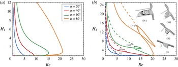
1 Introduction
Film flows, which are driven by a body force (such as gravity or the centrifugal force), the motion of the substrate itself or even by surface tension gradients, can be encountered in various engineering applications (Craster & Matar Reference Craster and Matar2009) such as spin coating (Stillwagon & Larson Reference Stillwagon and Larson1990), gravure printing (Yin & Kumar Reference Yin and Kumar2006; Grau et al. Reference Grau, Cen, Kang, Kitsomboonloha, Scheideler and Subramanian2016) or flows in two-phase heat exchangers and absorption or distillation columns using structured packings (Argyriadi, Vlachogiannis & Bontozoglou Reference Argyriadi, Vlachogiannis and Bontozoglou2006). In practice, however, the substrates encountered are never completely flat since they may contain well-defined features in the form of sharp steps, trenches, pillars, corrugations, etc. while irregularities may also arise due to the presence of arrested drops and particles on the substrate. Besides thickness variations of the coated layer, the presence of these topographic features may also lead to air entrapment inside them under certain conditions, e.g. for very deep trenches or trenches with enhanced hydrophobicity, which, in turn, may affect significantly the flow dynamics as well as the resulting coating quality of the solid surface.
The flow of a liquid film over topographical features has drawn the attention of many researchers over the years; an informative review of the literature can be found in Lampropoulos, Dimakopoulos & Tsamopoulos (Reference Lampropoulos, Dimakopoulos and Tsamopoulos2016). The most studied case is the one that corresponds to the desired arrangement in many coating applications where the liquid fully wets the solid structure; this wetting state is also known as the Wenzel state. A number of theoretical (Kalliadasis, Bielarz & Homsy Reference Kalliadasis, Bielarz and Homsy2000; Mazouchi & Homsy Reference Mazouchi and Homsy2001; Gaskell et al. Reference Gaskell, Jimack, Sellier, Thompson and Wilson2004; Wierschem & Aksel Reference Wierschem and Aksel2004; Bontozoglou & Serifi Reference Bontozoglou and Serifi2008; Heining et al. Reference Heining, Bontozoglou, Aksel and Wierschem2009; Nguyen & Bontozoglou Reference Nguyen and Bontozoglou2011) as well as experimental works (Decre & Baret Reference Decre and Baret2003; Argyriadi et al. Reference Argyriadi, Vlachogiannis and Bontozoglou2006) have demonstrated that the presence of topographic features leads to thickness variations of the coated layer due to the effect of the capillary and inertia forces. The stability of Newtonian film flow over a step-down has been reported to linear two-dimensional (2-D) disturbances by Kalliadasis & Homsy (Reference Kalliadasis and Homsy2001) or through nonlinear transient simulations by Bielarz & Kalliadasis (Reference Bielarz and Kalliadasis2003). In applications the flowing material is often a polymer solution or a suspension of particles and its non-Newtonian properties introduce interesting phenomena affecting the flow arrangement, the film shape and the stability of the liquid flow, but such studies have only recently appeared. The first attempt has been made by Saprykin, Koopmans & Kalliadasis (Reference Saprykin, Koopmans and Kalliadasis2007), who introduced small liquid elasticity and used the long-wave approximation, while more detailed analyses have appeared more recently (Pavlidis, Dimakopoulos & Tsamopoulos Reference Pavlidis, Dimakopoulos and Tsamopoulos2010; Pavlidis et al. Reference Pavlidis, Karapetsas, Dimakopoulos and Tsamopoulos2016).
As was mentioned above, a fully wetting state cannot always be achieved and in many cases air may become entrapped inside the topographical features, i.e. during the filling process. This often poses significant problems when for example it is desired to coat with a uniform photoresist layer a wafer surface with significant topography structures (Huang & Wang Reference Huang and Wang2014) or during cell filling with ink in gravure printing (Grau et al. Reference Grau, Cen, Kang, Kitsomboonloha, Scheideler and Subramanian2016). On the other hand, air entrapment can be highly desired in applications where drag reduction is required and one characteristic example is the flow over a super-hydrophobic surface (Ou & Rothstein Reference Ou and Rothstein2005). It is well known that the remarkable water repellent properties of these surfaces may not be caused by their surface chemistry alone, but also by the micro- or nanoscale surface structures (Cottin-Bizonne et al. Reference Cottin-Bizonne, Barrat, Bocquet and Charlaix2003; Quéré Reference Quéré2008; Bhushan, Jung & Koch Reference Bhushan, Jung and Koch2009). The presence of gas pockets trapped inside these structures leads to limited contact between the liquid and the solid surface enhancing the mobility of the liquid; this wetting state is known as the Cassie–Baxter state. As a result, when liquid flows over such surfaces the apparent slip length may become significantly enhanced; see the informative review by Rothstein (Reference Rothstein2010). It has been shown experimentally and theoretically that the Cassie state reduces the drag force on the liquid (Ou, Perot & Rothstein Reference Ou, Perot and Rothstein2004; Moulinet & Bartolo Reference Moulinet and Bartolo2007; Bonn et al. Reference Bonn, Eggers, Indekeu, Meunier and Rolley2009).
Theoretical efforts to account for the presence of air in the microstructure have focused mainly on idealized situations where it is often assumed that the liquid–gas interface is perfectly flat and/or pinned at the edges of the microstructure, i.e. assuming an ideal Cassie–Baxter state (Busse et al. Reference Busse, Sandham, Mchale and Newton2013; Park et al. Reference Park, Park, Lim and Kim2013; Hodes et al. Reference Hodes, Lam, Cowley, Enright and Maclachlan2015). Using this approach, factors such as the effect of the direction of flow with respect to structure topography have been investigated by examining grooves arranged either transversely or longitudinally to the flow (Davies et al. Reference Davies, Maynes, Webb and Woolford2006; Maynes et al. Reference Maynes, Jeffs, Woolford and Webb2007; Belyaev & Vinogradova Reference Belyaev and Vinogradova2010). Such idealized considerations, however, only reveal part of the story and in many cases may simply not be sufficient, e.g. due to the non-negligible effect of a curved liquid–gas interface or due to the partial penetration of the liquid in the microstructure; this is supported both by experimental observations (Tsai et al. Reference Tsai, Peters, Pirat, Wessling, Lammertink and Lohse2009) and numerical studies (Gao & Feng Reference Gao and Feng2009; Teo & Khoo Reference Teo and Khoo2010). The shape of the meniscus over the trench can be significantly affected, e.g. by the absolute pressure in the microchannel (Dilip, Bobji & Govardhan Reference Dilip, Bobji and Govardhan2015). Moreover, the meniscus stability, as well as the longevity of the gas pockets, were found by Byun et al. (Reference Byun, Kim, Ko and Park2008) to be very sensitive, under the same flow conditions, to the various geometrical characteristics. It has also been suggested that the longevity of the gas pockets can be affected by possible gas dissolution in the liquid phase (Lv et al. Reference Lv, Xue, Shi, Lin and Duan2014; Xiang et al. Reference Xiang, Xue, Lv, Li and Duan2016).
In order to examine the conditions leading to partially or fully non-wetted topographical features (Mazouchi, Gramlich & Homsy Reference Mazouchi, Gramlich and Homsy2004) studied the gravity-driven viscous flow over a flat plane with a moving contact line, while (Gramlich, Mazouchi & Homsy Reference Gramlich, Mazouchi and Homsy2004) investigated the time-dependent 2-D flow of a Newtonian film over orthogonal trenches. These authors assumed Stokes flow and produced flow maps of the various coating patterns which were found to depend on the trench width and depth as well as the substrate wettability. More recently, Lampropoulos et al. (Reference Lampropoulos, Dimakopoulos and Tsamopoulos2016) examined the same problem, albeit using the volume-of-fluid (VOF) method which enabled the investigation of cases with more complex dynamics, such as film pinching and merging or liquid impact on the solid wall in addition to perfect Cassie and Wenzel states, while taking fully into account the effect of liquid inertia. This work was extended by Karapetsas et al. (Reference Karapetsas, Lampropoulos, Dimakopoulos and Tsamopoulos2017), who reported coating patterns over three-dimensional topographical features via 3-D transient simulations. Here the flow maps are significantly affected also by the transverse dimension of the trench and the transverse distance between trenches. Both Lampropoulos et al. (Reference Lampropoulos, Dimakopoulos and Tsamopoulos2016) and Karapetsas et al. (Reference Karapetsas, Lampropoulos, Dimakopoulos and Tsamopoulos2017) found that, for deep enough trenches and depending on the substrate hydrophobicity, the film fails to wet the bottom of the trench. Moreover, these geometries arise in microelectromechanical devices (MEMs), in which experiments reveal that the liquid fails to cover completely the trench during spin coating, for example, and as a result air is entrapped inside this topography (Qianwen, Cui & Zheyao Reference Qianwen, Cui and Zheyao2012).
Transient simulations are quite expensive and unable to cover adequately the multidimensional parameter space in this problem. This can be remedied by steady-state calculations. These will also definitively demonstrate that the widely used ideal Cassie state is not the only possible or the preferred arrangement, something that has been routinely assumed, especially when the substrate is hydrophobic. To this end, we will develop a more accurate solution methodology to compute the interface not only outside the slit, but also the second interface inside it, irrespective of the often large deformations that it undergoes and the space it provides for developing multiple zones of liquid recirculation. Thus, we will determine complete families of steady solutions and their dependence on all the parameters of this problem. In most cases a hydrodynamic hysteresis will be found for specific values of the Weber number. This is similar to the findings by Kistler & Scriven (Reference Kistler and Scriven1994), who examined the teapot effect, but is unrelated to the well-known contact angle hysteresis. The resulting family of shapes indicates that abrupt changes in the flow patterns are possible via small changes in the relevant parameter and, equally importantly, that certain predicted stable steady states may be attainable only via careful inception of flow. Another objective of this work is to examine whether the Gibbs inequality limits the extent of solution families in the presence of this flow. This numerical effort has been supplemented by simplified force balances, which provide the correct scales and help in determining conditions under which critical points in the solution families collapse, irrespective of the liquid or the contact angle employed. With this procedure we will examine in more detail the possible arrangements of a liquid film flowing over an inclined substrate featuring a slit. The slit does not have a bottom or its bottom may be at large enough distance from the outer substrate surface, as in porous materials and superhydrophobic surfaces, so that it is not wet by the liquid. In this way the liquid may wet at any distance the slit without the positive or negative action of the bottom.
This paper is organized as follows. In § 2 the problem formulation along with the governing equations is given, and the numerical implementation is briefly presented in § 3. The discussion of the results from our numerical simulations for either hydrophilic or hydrophobic surfaces follows and the effects of inertia, viscous, capillary and gravitational forces along with substrate orientation and slit width are presented in § 4. Conclusions are drawn in § 5.
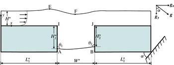
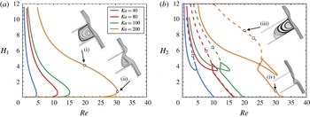
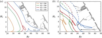
Cross-section of the film flowing over a substrate inclined with respect to the horizontal by an angle
 $\unicode[STIX]{x1D6FC}$
and featuring a slit.
 $L_{1}^{\ast }$
and
 $L_{2}^{\ast }$
are the entrance and exit lengths before and after the slit, respectively,
 $W^{\ast }$
is the slit width,
 $H^{\ast }$
is the film height at the inlet,
 $H_{1}^{\ast }$
and
 $H_{2}^{\ast }$
are the distances from the respective corners of the contact lines along the upstream and downstream slit walls, E and F are the locations of the maximum and minimum outer film interface, if they arise.

2 Problem formulation
We consider the steady, free-surface flow of a liquid film driven by gravity along a planar solid substrate featuring a slit normal to the main flow direction. The liquid is Newtonian and incompressible, with constant density
 $\unicode[STIX]{x1D70C}$
, dynamic viscosity
 $\unicode[STIX]{x1D707}$
and interfacial tension
 $\unicode[STIX]{x1D70E}$
. A cross-section of the substrate and the film is given in figure 1, which also depicts the geometric characteristics of the substrate and the film. The primitive flow input is the volumetric flow rate per unit length normal to the cross-section,
 $Q^{\ast }$
. In what follows, a superscript ‘*’ will indicate a dimensional quantity. Under gravity, the liquid film flows downward along the substrate and may partially enter the slit, forming two interfaces with the air: the usual one over the substrate and outside the slit and a second one inside it. Under these conditions, the air inside the slit is at ambient pressure. Both free surfaces are taken as shear free, i.e. the dynamic effect of the adjacent gas phase is negligible. The inner interface intersects the side walls of the slit defining two horizontal contact lines. In the depicted cross-section, the two contact lines are represented by the two points, A and B. Their locations are determined by liquid properties and flow conditions along with the apparent contact angles
 $\unicode[STIX]{x1D703}_{1}$
and
 $\unicode[STIX]{x1D703}_{2}$
, respectively. These are the angles between the solid wall and the visible free surface at a putative contact line. Hence, each contact line can translate along each side of the slit up to the corresponding slit edge. At the contact line, a sudden change occurs from adherence at a solid surface to no shear along a free surface inducing a local logarithmic singularity, which is proved to be integrable (Michael Reference Michael1958; Richardson Reference Richardson1970). So the apparent contact angle is accepted as an overall measure of the solid wettability (Kistler & Scriven Reference Kistler and Scriven1994).
We take a Cartesian coordinate system with origin in the flow entrance and the
 $x$
-axis in the direction parallel to the wall and the
 $y$
-axis outward pointing and normal to the wall, as indicated in figure 1. The two-dimensional steady-state flow is governed by conservation equations for mass, equation (2.1), and momentum, equation (2.2), which, in dimensionless form, are given by,
 $$\begin{eqnarray}\displaystyle & \displaystyle \unicode[STIX]{x1D735}\boldsymbol{\cdot }\boldsymbol{v}=0, & \displaystyle\end{eqnarray}$$
 $$\begin{eqnarray}\displaystyle & \displaystyle Re(\boldsymbol{v}\boldsymbol{\cdot }\unicode[STIX]{x1D735}\boldsymbol{v})+\unicode[STIX]{x1D735}P-\unicode[STIX]{x1D6FB}^{2}\boldsymbol{v}-St\,\boldsymbol{g}=0, & \displaystyle\end{eqnarray}$$
where
 $\boldsymbol{v}=(v_{x},v_{y})^{\text{T}}$
and
 $P$
are the dimensionless velocity vector and the pressure, and
 $\boldsymbol{g}=(\sin \unicode[STIX]{x1D6FC},-\text{cos}\unicode[STIX]{x1D6FC})^{\text{T}}$
is the unit vector in the direction of gravity. In the above and heretofore, the velocity and length scales are the average velocity
 $U^{\ast }$
and the film thickness
 $H^{\ast }$
at the entrance, respectively. In general the viscous scale (
 $\unicode[STIX]{x1D707}U^{\ast }/H^{\ast }$
) is used for scaling pressure. Thus, the dimensionless groups that arise are the Reynolds and the Stokes numbers,
 $$\begin{eqnarray}Re\equiv \frac{\unicode[STIX]{x1D70C}U^{\ast }H^{\ast }}{\unicode[STIX]{x1D707}},\quad St\equiv \frac{\unicode[STIX]{x1D70C}gH^{\ast 2}}{\unicode[STIX]{x1D707}U^{\ast }}.\end{eqnarray}$$
Considering that in applications a sequence of parallel slits arises, we impose flow periodicity between the inlet and the outlet of the examined domain. Therefore, the flow at the entrance and exit is not necessarily a Nusselt flat film flow, so
 $U^{\ast }$
cannot be directly related to
 $H^{\ast }$
or
 $Q^{\ast }$
. On the other hand, provided that the entrance and exit lengths are long enough, so that the outer interface is flat there, irrespective of the size of the slit and flow and liquid parameters, the Nusselt flat film flow would be approached there and thus the velocity and length scales would approximate the characteristic Nusselt scales,
 $$\begin{eqnarray}U_{N}^{\ast }=Q^{\ast 2/3}\left(\frac{\unicode[STIX]{x1D70C}g\sin (\unicode[STIX]{x1D6FC})}{3\unicode[STIX]{x1D707}}\right)^{1/3},\quad H_{N}^{\ast }=Q^{\ast 1/3}\left(\frac{3\unicode[STIX]{x1D707}}{\unicode[STIX]{x1D70C}g\sin (\unicode[STIX]{x1D6FC})}\right)^{1/3}.\end{eqnarray}$$
If the Nusselt length and velocity scales had been used,
 $St_{N}=3/\text{sin}(\unicode[STIX]{x1D6FC})$
. Here however,
 $St$
is determined by imposing the dimensionless flow rate at the entrance or the dimensionless mean velocity to be unity,
 $$\begin{eqnarray}Q\equiv \int _{0}^{1}v_{x}\,\text{d}y=1.\end{eqnarray}$$
For the simulation that will be presented below, we have chosen the domain inlet and outlet lengths to be large enough, typically
 $L_{1}=L_{2}=20$
, and the Nusselt film flow is expected to hold at the entrance and exit planes. If a small deviation of
 $St$
from its Nusselt value,
 $St_{N}$
, arises, it indicates the extent to which the presence of the slit has affected the inflow and outflow boundaries.
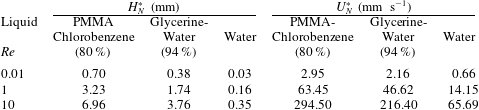
Properties of typical liquids.

Along the two air–liquid interfaces we apply a normal stress balance, between capillary force and viscous stress, while we impose a zero tangential stress. We set the ambient air pressure,
 $P_{a}$
, equal to zero as the datum pressure,
 $$\begin{eqnarray}\boldsymbol{n}\boldsymbol{\cdot }\unicode[STIX]{x1D64F}=-P_{a}\,\boldsymbol{n}+\frac{2H_{\text{m}}}{Ca}\,\boldsymbol{n},\end{eqnarray}$$
In the above, the total stress tensor is defined as
 $\unicode[STIX]{x1D64F}=-P\unicode[STIX]{x1D644}+(\unicode[STIX]{x1D735}\boldsymbol{v}+(\unicode[STIX]{x1D735}\boldsymbol{v})^{\text{T}})$
,
 $\boldsymbol{n}$
is the unit vector normal to either air–liquid interface pointing outward with respect to the film, the mean curvature is
 $2H_{m}=-\unicode[STIX]{x1D735}_{s}\boldsymbol{\cdot }\boldsymbol{n}$
, with
 $\unicode[STIX]{x1D735}_{s}=(\unicode[STIX]{x1D644}-\boldsymbol{n}\boldsymbol{n})\boldsymbol{\cdot }\unicode[STIX]{x1D735}$
. The capillary number,
 $Ca\equiv \unicode[STIX]{x1D707}U^{\ast }/\unicode[STIX]{x1D70E}$
, arises naturally in (2.6), but it is dropped in favour of the Kapitza number,
 $$\begin{eqnarray}Ka=\frac{\unicode[STIX]{x1D70E}\unicode[STIX]{x1D70C}^{1/3}}{g^{1/3}\unicode[STIX]{x1D707}^{4/3}}=\left(\frac{l_{c}^{\ast }}{l_{v}^{\ast }}\right)^{2},\end{eqnarray}$$
because the latter depends exclusively on liquid properties or, equivalently, the ratio of the capillary length,
 $l_{c}^{\ast }$
, to the viscous length,
 $l_{v}^{\ast }$
, defined as
 $$\begin{eqnarray}l_{c}^{\ast }\equiv \left(\frac{\unicode[STIX]{x1D70E}}{\unicode[STIX]{x1D70C}g}\right)^{1/2},\quad l_{v}^{\ast }\equiv \left(\frac{\unicode[STIX]{x1D707}^{2}}{\unicode[STIX]{x1D70C}^{2}g}\right)^{1/3}.\end{eqnarray}$$
We should mention here that the Kapitza number varies primarily due to variations in liquid viscosity, because surface tension and density of most common liquids vary in a much shorter range, see also table 1. Clearly
 $Ka$
is not an independent number, but is related to the previously defined dimensionless quantities via the expression
 $$\begin{eqnarray}Ka=Ca^{-1}St^{-1/3}Re^{2/3}.\end{eqnarray}$$
In the results section it will become clear that two more dimensionless numbers are relevant for the analysis. One is the Weber number, which is a measure of liquid inertia to its capillary force. Based on the chosen characteristic scales, it is defined as,
 $$\begin{eqnarray}We=\frac{\unicode[STIX]{x1D70C}U^{\ast 2}H^{\ast }}{\unicode[STIX]{x1D70E}}\equiv Re\,Ca\end{eqnarray}$$
and the other is the Bond number, which is a measure of the gravitational to capillary force, defined as,
 $$\begin{eqnarray}Bo=\frac{\unicode[STIX]{x1D70C}gH^{\ast 2}}{\unicode[STIX]{x1D70E}}=St\;Ca.\end{eqnarray}$$
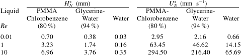
Noting that the flow examined can appear in a variety of applications ranging from film coating with polymeric solutions to water flow over superhydrophobic surfaces, we present in table 1 the properties, and
 $l_{c}^{\ast }$
,
 $l_{v}^{\ast }$
,
 $Ka$
for three typical liquids. Combining these properties with a flow rate determines Re via (2.3) and the Nusselt film thickness,
 $H_{N}^{\ast }$
, and the mean velocity,
 $U_{N}^{\ast }$
, via (2.4), which are given in table 2 or alternatively the film thickness in the entrance via the expression
 $(H^{\ast }/l_{v}^{\ast })^{3}=Re\;St$
.
Variation of Nusselt thickness and velocity for the three liquids for different
 $Re$
, at
 $\unicode[STIX]{x1D6FC}=60^{\circ }$
.
Under steady-state conditions, the two gas–liquid interfaces are impenetrable and obey the reduced kinematic condition,
 $$\begin{eqnarray}\boldsymbol{u}\boldsymbol{\cdot }\boldsymbol{n}=0.\end{eqnarray}$$
At the two intersections of the inner interface (its unit normal vectors denoted as
 $\boldsymbol{n}_{s1}$
,
 $\boldsymbol{n}_{s2}$
) with the two side walls of the slit (their unit normal vectors denoted as
 $\boldsymbol{n}_{w1}$
,
 $\boldsymbol{n}_{w2}$
), the contact angles are imposed allowing the corresponding contact lines to find their static positions,
 $$\begin{eqnarray}\displaystyle & \displaystyle \boldsymbol{n}_{w1}\boldsymbol{\cdot }\boldsymbol{n}_{s1}=\cos \unicode[STIX]{x1D703}_{1}, & \displaystyle\end{eqnarray}$$
 $$\begin{eqnarray}\displaystyle & \displaystyle \boldsymbol{n}_{w2}\boldsymbol{\cdot }\boldsymbol{n}_{s2}=\cos \unicode[STIX]{x1D703}_{2}, & \displaystyle\end{eqnarray}$$
In the results section, it will become apparent that the flow inside the slit is much slower than the film flow (often the velocity magnitude in the slit is orders of magnitude smaller) and that one or more counter-rotating vortices may arise there. Hence, the contact angles at points A and B may have the tendency to be either receding or advancing, albeit with a very small velocity in their vicinity. Therefore, it is reasonable to neglect this tendency and assume them to have the same value
 $\unicode[STIX]{x1D703}$
, characterizing the specific solid/liquid pair, i.e. we set
 $\unicode[STIX]{x1D703}_{1}=\unicode[STIX]{x1D703}_{2}=\unicode[STIX]{x1D703}$
. This also reduces the number of parameters in our analysis. Moreover, the no-slip and no-penetration conditions are imposed along the solid boundary. Unless stated otherwise, throughout the paper the dimensionless width of the slit is set at
 $W=5$
, noting that its corresponding dimensional value will vary proportionally to the film thickness at the entrance, which has been chosen as the length scale.
3 Numerical implementation
In order to solve numerically the above set of equations we have chosen the mixed finite element method to discretize the velocity and pressure fields combined with a quasi-elliptic grid generation scheme for the tessellation of the deformed physical domain.
3.1 Elliptic grid generation
The grid generation scheme consists of a system of quasi-elliptic partial differential equations, capable of generating a boundary fitted tessellation of the deforming domain occupied by the liquid. Here we will only present our adaptation of its essential features to the current problem. The interested reader may refer to Dimakopoulos & Tsamopoulos (Reference Dimakopoulos and Tsamopoulos2003) for further details. With this scheme the physical domain
 $(x,y)$
is mapped onto a computational one
 $(\unicode[STIX]{x1D709},\unicode[STIX]{x1D702})$
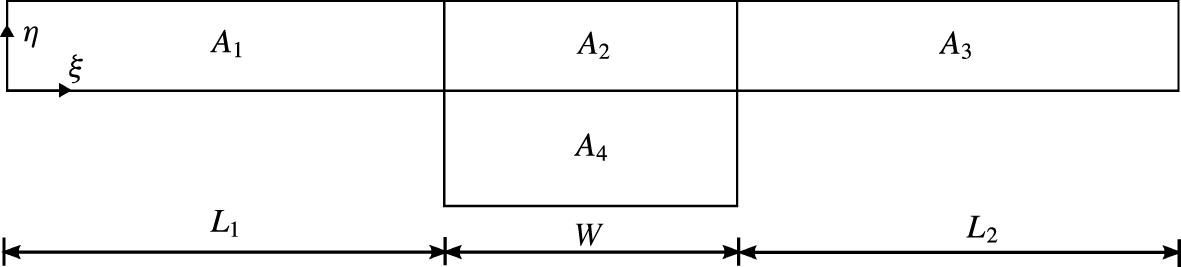
. A fixed computational mesh is generated in the latter domain while, through the mapping, the corresponding mesh in the physical domain follows its deformations. As computational domain we choose here the entire volume that would be occupied by the liquid, if the two interfaces were flat, see figure 2.
The computational domain is decomposed into four subdomains,
 $A_{1},A_{2},A_{3}$
corresponding to the outer film and
 $A_{4}$
corresponding to the liquid inside the slit. This decomposition allows us to strongly enforce the location of the nodes in their common boundaries and their adjustment depending on the liquid penetration in the slit.

This mapping is based on the solution of the following system of quasi-elliptic partial differential equations
 $$\begin{eqnarray}\displaystyle & \displaystyle \unicode[STIX]{x1D735}\boldsymbol{\cdot }\left\{\left[\unicode[STIX]{x1D700}\sqrt{\frac{x_{\unicode[STIX]{x1D702}}^{2}+y_{\unicode[STIX]{x1D702}}^{2}}{x_{\unicode[STIX]{x1D709}}^{2}+y_{\unicode[STIX]{x1D709}}^{2}}}+(1-\unicode[STIX]{x1D700})\right]\unicode[STIX]{x1D735}\unicode[STIX]{x1D709}\right\}=0, & \displaystyle\end{eqnarray}$$
 $$\begin{eqnarray}\displaystyle & \displaystyle \unicode[STIX]{x1D6FB}^{2}\unicode[STIX]{x1D702}=0, & \displaystyle\end{eqnarray}$$
the unknowns of which are the coordinates of the nodes in physical space
 $\boldsymbol{x}=(x,y)$
, subscripts denote differentiation with respect to the indicated variable and
 $\unicode[STIX]{x1D700}$
is a parameter that controls the smoothness of the mapping relative to the degree of orthogonality of the mesh lines; here
 $\unicode[STIX]{x1D700}=0.1$
. In order to solve the above system of differential equations, appropriate boundary conditions must be imposed; see Dimakopoulos & Tsamopoulos (Reference Dimakopoulos and Tsamopoulos2003). To prevent larger element distortion, we split the domain into the four subdomains shown in figure 2 and we impose node equidistribution on the boundaries between the subdomains
 $A_{1}-A_{2},\;A_{2}-A_{3}$
and
 $A_{2}-A_{4}$
. The rectangular elements generated with this procedure are further split in half, producing triangular elements, because the latter conform better to the large deformations of the physical domain and can sustain larger distortions than the rectangular ones.
3.2 Mixed finite element method
We approximate the velocity and position vector, with 6-node Lagrangian basis functions in the triangular elements,
 $\unicode[STIX]{x1D719}^{i}$
, and the pressure with 3-node Lagrangian basis functions,
 $\unicode[STIX]{x1D713}^{i}$
:
 $$\begin{eqnarray}\boldsymbol{v}=\mathop{\sum }_{k=1}^{6}\boldsymbol{v}_{k}\unicode[STIX]{x1D719}^{k}(\unicode[STIX]{x1D709},\unicode[STIX]{x1D702}),\quad \boldsymbol{x}\,=\mathop{\sum }_{k=1}^{6}\boldsymbol{x}_{k}\unicode[STIX]{x1D719}^{k}(\unicode[STIX]{x1D709},\unicode[STIX]{x1D702}),\quad P\,=\mathop{\sum }_{l=1}^{3}p_{l}\unicode[STIX]{x1D713}^{l}(\unicode[STIX]{x1D709},\unicode[STIX]{x1D702}).\end{eqnarray}$$
For the momentum and mass balances as well as the mesh generation equations we employ the finite element/Galerkin method, which after applying the divergence theorem reduces them into their corresponding weak forms. The number of the residuals of the resulting equations equals the number of the nodal unknown variables
 $v_{x}^{i},\;v_{y}^{i},\;P^{i},\;x^{i}$
and
 $y^{i}$
(denoted by a global unknown vector
 $\boldsymbol{q}$
). The unknowns are computed via the Newton–Raphson method and the Jacobian matrix is numerically evaluated by first-order finite difference approximation.
As will become apparent in the results section, multiple steady solutions may arise for the same parameter value, which are connected via limit points. This precludes using the zeroth- or first-order continuation method to trace such a solution family. To do so, the pseudo arclength continuation technique is incorporated into the finite element code (Fraggedakis et al.
Reference Fraggedakis, Pavlidis, Dimakopoulos and Tsamopoulos2016). Given a solution,
 $\boldsymbol{q}_{0}$
, at an initial parameter value, say
 $\unicode[STIX]{x1D706}_{0}$
, the value of the parameter
 $\unicode[STIX]{x1D706}$
, for the next computation is determined as a function of the pseudo arclength,
 $s$
, along the curve of solutions. In order to determine
 $\unicode[STIX]{x1D706}$
, an additional equation is obtained by projecting the increment of the augmented solution vector
 $(\boldsymbol{q}-\boldsymbol{q}_{0},\unicode[STIX]{x1D706}-\unicode[STIX]{x1D706}_{0})^{\text{T}}$
on its initial tangent
 $(\dot{\boldsymbol{q}}_{0},\dot{\unicode[STIX]{x1D706}}_{0})^{\text{T}}$
, where the derivatives are taken with respect to the parameter
 $s$
. The product is set equal to a specified arclength
 $\unicode[STIX]{x0394}s$
resulting in the additional equation (3.4),
 $$\begin{eqnarray}G(\boldsymbol{q},\unicode[STIX]{x1D706};\unicode[STIX]{x0394}s):=\dot{\boldsymbol{q}}_{0}^{\text{T}}\boldsymbol{\cdot }(\boldsymbol{q}-\boldsymbol{q}_{0})+\dot{\unicode[STIX]{x1D706}}_{0}(\unicode[STIX]{x1D706}-\unicode[STIX]{x1D706}_{0})+\unicode[STIX]{x0394}s=0.\end{eqnarray}$$
In summary, we need to solve the following augmented system of equations (3.5) and (3.6) for the augmented solution vector
 $(\boldsymbol{q},\unicode[STIX]{x1D706})^{\text{T}}$
,
 $$\begin{eqnarray}\displaystyle & \displaystyle \boldsymbol{F}(\boldsymbol{q},\unicode[STIX]{x1D706})=0, & \displaystyle\end{eqnarray}$$
 $$\begin{eqnarray}\displaystyle & \displaystyle G(\boldsymbol{q},\unicode[STIX]{x1D706};\unicode[STIX]{x0394}s)=0, & \displaystyle\end{eqnarray}$$
where
 $\boldsymbol{F}$
is the system of weighted governing and mesh generating equations, including the extra equation (2.5). The extended solution is first predicted as follows,
 $$\begin{eqnarray}\displaystyle & \displaystyle \boldsymbol{q}=\boldsymbol{q}_{0}+\unicode[STIX]{x0394}s\,\dot{\boldsymbol{q}}_{0}, & \displaystyle\end{eqnarray}$$
 $$\begin{eqnarray}\displaystyle & \displaystyle \unicode[STIX]{x1D706}=\unicode[STIX]{x1D706}_{0}+\unicode[STIX]{x0394}s\,\dot{\unicode[STIX]{x1D706}}_{0}, & \displaystyle\end{eqnarray}$$
and then the system of equations is solved by the Newton–Raphson iteration method. The Jacobian of the system of equations is a sparse matrix that can be stored by three single-index arrays following the compressed sparse row (CSR) format and solved with a sparse matrix solver (Gupta 2000), except for the two extra equations (2.5) and (3.4), which produce more entries in the Jacobian and in different locations. This destroys the sparsity and structure of the Jacobian in the CSR format, if incorporated into the previous system and solved simultaneously. The way out is to apply the special algebraic procedure described in Zacharioudaki et al. (Reference Zacharioudaki, Kouris, Dimakopoulos and Tsamopoulos2007) to solve first for the two extra global variables, which are the Stokes number and the unknown value of the parameter in the arclength continuation.
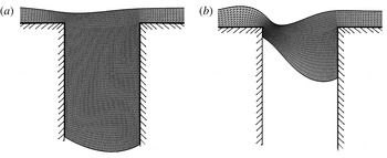
Close-up views of the mesh in the vicinity of the slit, demonstrating the quality of the structured mesh that is produced. The widely different interface shapes obtained during parameter continuation require adjusting the number of elements in the slit and interpolating the variables to the new mesh to keep the high mesh quality, with a low computational cost: (a) large liquid penetration in the slit with
 $Re=3$
; (b) smaller liquid penetration with
 $Re=15.25$
. The other parameter values are
 $\unicode[STIX]{x1D703}=120^{\circ }$
,
 $Ka=100,W=5$
and
 $\unicode[STIX]{x1D6FC}=60^{\circ }$
.

Another crucial feature of this partial liquid penetration problem is that the physical domain is not confined, but it freely expands or shrinks inside the slit during parameter continuation and the two contact points translate quite independently. When the wetting distance increases, the number of elements inside the slit should increase proportionately. For example, the number of elements in the
 $y$
-direction for the part of the computational domain inside the slit gradually changes from 60 quadrilateral elements for a deep wetting in figure 3(a) to 16 quadrilateral elements for shallow wetting with quite distorted inner interface in figure 3(b). In order to take these deformations into account, we split the computational domain into two parts: a rectangular one, mapping the outer flow (subdomains
 $A_{1},A_{2},A_{3}$
in figure 2), and another one for the liquid inside the slit, which is resolved by adapting the mesh to its variations (subdomain
 $A_{4}$
). When the wetting length along the upstream wall vanishes and contact point A coincides with the upstream corner, the same decomposition into subdomains is used, but the side corresponding to the upstream slit wall in the computational domain is used to describe part of the inner free surface. When both wetting lengths vanish, subdomain
 $A_{4}$
is not used. Despite the high quality of the mesh for a given set of parameter values, the large variations of slit wetting results in large deformations of the mesh in physical space. To deal with the large aspect ratios of the elements, a remeshing procedure was developed along with the domain decomposition method during which elements are added to or subtracted from subdomain
 $A_{4}$
, following the ideas in Dimakopoulos & Tsamopoulos (Reference Dimakopoulos and Tsamopoulos2009), Papaioannou et al. (Reference Papaioannou, Giannousakis, Dimakopoulos and Tsamopoulos2014). Parameter continuation is halted and complete mesh reconstruction is performed, when mesh deformation exceeds a certain level. The remeshing procedure is summarized in the following steps: (i) the last converged film shape is retained and a new selection of node positions in the inner interface is made with nodes that are equidistributed along the inner boundary curve. (ii) The new mesh is generated in the bulk of the film with essential conditions the previously determined nodes on the boundaries. (iii) The flow variables (velocities and pressure) are calculated on the new nodes of the physical domain from the old ones using search and finite element interpolation techniques.
The usual tests of solution convergence with mesh refinement have been performed to determine the optimum mesh to use in terms of computational accuracy and cost. In this regard, attention has been paid in the accuracy achieved in calculating the pressure variable close to the points it is expected to be singular, i.e. the entrance and exit corners to the slit and the contact points. For example, according to Dean & Montagnon (Reference Dean and Montagnon1949) pressure is singular at a
 $270^{\circ }$
corner (the entrance and exit slit corners), where the strongest singularity is
 $r^{-0.456}$
, where
 $r$
is the distance from the corner. It has been shown by Georgiou, Schultz & Olson (Reference Georgiou, Schultz and Olson1990) that this singularity affects the solution only locally and can be treated either by special ‘singular’ elements or by mesh refinement. We have verified that with the mesh we have chosen pressure oscillations are confined to only 2–3 elements away from each corner, i.e. up to
 ${\sim}0.1$
radius around the corner, but do not affect the rest of the solution in any way.
4 Results and discussion
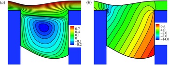
Figure 4 depicts representative flow and pressure fields and especially their part inside and around the slit. The minimum in the outer interface appears close to the upstream corner, locally decreasing the flow cross-section and contributing to the larger flow intensification there in comparison to that in the downstream corner. The pressure variation inside the slit increases the curvature of the inner surface closer to contact point B, but does not change its sign in this case. The contours of both variables are smooth, even close to the slit corners or the contact points, attesting to the accuracy of the computations.
Close-up views of the streamlines (a) and pressure field (b) for
 $Re=7$
,
 $Ka=100$
,
 $\unicode[STIX]{x1D703}=120^{\circ }$
, at inclination angle
 $\unicode[STIX]{x1D6FC}=60^{\circ }$
and slit width
 $W=5$
. Flow is from left to right.

The streamlines indicate that there is a region close to the inner interface, where
 $v_{x}$
is negative, while
 $v_{y}$
changes from positive near the upstream wall to negative near the downstream wall indicating a recirculation. This reverse flow is bounded in this case between the inner interface and a curve intersecting the two slit walls near their respective corners. The recirculation keeps the liquid within this region and detaches it from the film flowing along the outer interface. Hence, the liquid inside the slit can be separated into two zones: the one closer to the outer interface, which has positive
 $v_{x}$
and its motion is driven by Nusselt-type flow upstream and downstream the slit and the other up to the inner interface, which undergoes recirculation. Note that, because of the recirculation, the liquid motion near the contact point A would promote liquid receding, while near the contact point B liquid advancing, i.e. opposite to what would prevail without recirculation. Moreover the velocity magnitude in the recirculation region is often more than an order of magnitude smaller than in the outer film (see figure 4 and results to follow). These are the reasons we took
 $\unicode[STIX]{x1D703}_{1}=\unicode[STIX]{x1D703}_{2}=\unicode[STIX]{x1D703}$
. In the pressure contours, (figure 4
b), we observe a maximum value of pressure near the contact point B and a minimum one at the step-in corner. For the most part, the contours of pressure inside the slit are normal to the direction of gravity. This implies that the pressure of the liquid inside the slit is mainly hydrostatic, which should have been anticipated given the very slow flow there.
An important classification of the results that will follow is based on this observation about the pressure inside the slit, which indicates that the flow intensity is considerably reduced resulting in subdominant viscous stresses with respect to the pressure. This allows simplification of the force balance on the inner interface, equation (2.6), to the hydrostatic Young–Laplace equation, which relates the pressure difference between the two adjacent phases to the curvature of the interface:
 $$\begin{eqnarray}\unicode[STIX]{x0394}P^{\ast }=2\unicode[STIX]{x1D70E}H_{m}^{\ast }\equiv \unicode[STIX]{x1D70E}\left(\frac{1}{R_{1}^{\ast }}+\frac{1}{R_{2}^{\ast }}\right),\end{eqnarray}$$
where
 $R_{1}^{\ast }$
and
 $R_{2}^{\ast }$
are the two radii of curvature. Under the assumption of constant curvature, which is valid for narrow enough slits,
 $R_{1}^{\ast }$
is related to the slit width,
 $W^{\ast }$
, and the contact angle via
 $R_{1}^{\ast }=(W^{\ast }/2)\,1/\cos (\unicode[STIX]{x1D703})$
, whereas
 $R_{2}^{\ast }=\infty$
in this Cartesian geometry. This pressure difference is balanced by the liquid weight inside the slit. The inclination of the substrate with respect to gravity will cause only a small difference between the two wetting lengths
 $H_{1}^{\ast }$
and
 $H_{2}^{\ast }$
, when
 $W^{\ast }$
is small. Hence, we can introduce, the average penetration of the liquid flow inside the slit as:
 $$\begin{eqnarray}h^{\ast }(a,\unicode[STIX]{x1D703})\equiv \frac{H_{1}^{\ast }+H_{2}^{\ast }}{2}=-\frac{\unicode[STIX]{x1D70E}}{\unicode[STIX]{x1D70C}g}\left(\frac{1}{W^{\ast }/2}\right)\frac{\cos (\unicode[STIX]{x1D703})}{\cos (\unicode[STIX]{x1D6FC})}.\end{eqnarray}$$
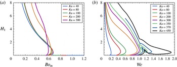
This equation, based on a force balance, indicates that, instead of the definition in (2.11), it is more appropriate to introduce the modified Bond number as follows:
 $$\begin{eqnarray}Bo_{m}=\frac{\unicode[STIX]{x1D70C}gH^{\ast }W^{\ast }}{\unicode[STIX]{x1D70E}}=Bo\;W\approx -\frac{\cos (\unicode[STIX]{x1D703})}{\cos (\unicode[STIX]{x1D6FC})}.\end{eqnarray}$$
According to (4.2)
 $h^{\ast }$
depends on the liquid properties, geometry and orientation of the substrate and finally its hydrophobicity and predicts that wetting is possible when the fraction
 $\cos (\unicode[STIX]{x1D703})/\text{cos}(\unicode[STIX]{x1D6FC})$
is negative. So, the inclination angle spectrum can be split into two groups. For inclination angles less than
 $90^{\circ }$
wetting is possible for hydrophobic substrates, while for inclination angles greater than
 $90^{\circ }$
finite wetting is possible for hydrophilic substrates.
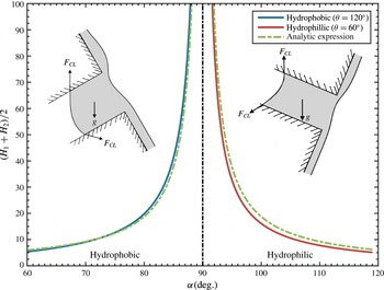
In figure 5 we present the computed dimensionless average wetting penetration as a function of the inclination angle for both hydrophobic and hydrophilic substrates for
 $Ka=100,Re=5$
and
 $W=5$
, in comparison to the analytical predictions of (4.2). Both for hydrophobic and hydrophilic substrates very good quantitative agreement is observed, especially for large penetration depths. Larger deviations arise when the penetration depth decreases, because in such cases the film in the slit interacts more strongly with the outer film flow and the assumption of hydrostatic pressure and very weak flow breaks down. Moreover, the wetting depth approaches infinity asymptotically when the inclination angle approaches
 $90^{\circ }$
. Clearly the same asymptote separates solutions over hydrophobic from those over hydrophilic substrates.
Average liquid penetration for hydrophobic surfaces (blue continuous line) and hydrophilic surfaces (red continuous line) in comparison with analytical expression from hydrostatics (green discontinuous lines). Flow parameters:
 $Ka=100$
,
 $Re=5$
,
 $W=5$
. Computing this very deep wetting required several remeshing and interpolation cycles during parameter continuation and, when the inclination angle approached
 $90^{\circ }$
, a very large number of elements in subdomain
 $A_{4}$
.

The physical interpretation of the asymptotic increase of the wetting length goes as follows: as the substrate tends to become vertical, the
 $y$
-component of gravity towards the slit becomes weaker. The vertical position, at
 $\unicode[STIX]{x1D6FC}=90^{\circ }$
, corresponds to capillary imbibition without any restraining force. Similarly, when the slit width decreases, the same capillary force can still balance the same liquid mass, which is obtained by increasing the wetting length. It is important to note that this analysis is based on the existence of a quasi-hydrostatic force balance. This balance cannot be satisfied, (i) for hydrophilic surfaces and
 $\unicode[STIX]{x1D6FC}<90^{\circ }$
, when both capillarity and gravity promote liquid penetration and are not balanced by any other force leading to continuous leaking of the liquid through the slit and (ii) for hydrophobic surfaces and
 $\unicode[STIX]{x1D6FC}>90^{\circ }$
, when both capillarity and gravity prevent liquid penetration leading to no wetting of the slit. These observations necessitate studying separately the wetting of hydrophobic from hydrophilic substrates.
In the following we will focus our presentation on film shapes inside and around the slit, quantify them via the depths of the two contact points and the variation of the outer surface and will discuss the flow field in particular cases via the corresponding streamline patterns.
4.1 Hydrophilic surfaces
4.1.1 General pattern
As explained previously, finite slit wetting of hydrophilic substrates takes place only for inclination angles larger than
 $90^{\circ }$
; here we discuss
 $\unicode[STIX]{x1D6FC}=100^{\circ }$
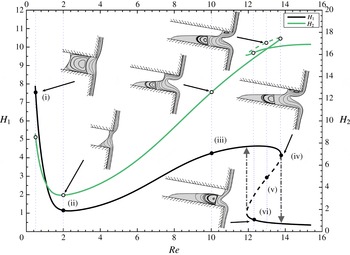
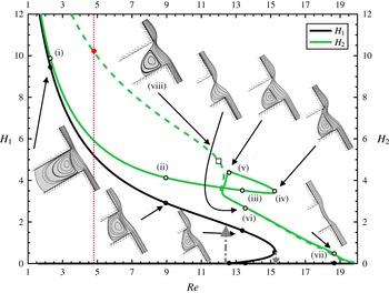
, as a base case. Figure 6 presents the effect of increasing the flow rate, via the proportionately increasing Reynolds number, on steady film flow along a substrate with contact angle
 $\unicode[STIX]{x1D703}=60^{\circ }$
for liquids with
 $Ka=15$
. The variation of the two wetting lengths,
 $H_{1}$
and
 $H_{2}$
, is shown along with a few representative film shapes and streamline patterns given as insets. The film entering the slit area generates a stagnation point in the downstream slit wall, which, through the locally increased pressure, forces the liquid either to change course exiting the slit or to get entrapped producing an eddy.
Dependence of the wetting lengths
 $H_{1}$
(black line, points marked
 $\bullet$
) and
 $H_{2}$
(green line, points marked
 $\circ$
) on the Reynolds number for
 $\unicode[STIX]{x1D703}=60^{\circ }$
and
 $Ka=15$
, at inclination angle
 $\unicode[STIX]{x1D6FC}=100^{\circ }$
. Continuous and discontinuous lines indicate stable and unstable solutions, respectively. The same curve types are used in similar figures that follow. The arrows indicate the ‘jumps’ in
 $H_{1}$
, when
 $Re$
exceeds the respective values at the two limit points forming the hysteresis loop.

First, we examine film flow with
 $Re\leqslant 2$
. Given that the material,
 $\unicode[STIX]{x1D703}$
and
 $\unicode[STIX]{x1D6FC}$
(hence
 $St$
and
 $Ka$
) remain constant, decreasing
 $Re$
to so small values means not only that inertia inside the slit decreases with respect to the viscous forces there, but also, through (2.9), that
 $Ca$
decreases as well and, hence, viscous forces decrease with respect to capillarity. Therefore, the only remaining force trying to maintain the liquid from draining out of the slit is capillarity. Its combined effect, through the curvature of the inner interface and the contact points, is balanced only by the small (due to the chosen inclination angle)
 $y$
-component of gravity. This makes
 $Bo_{m}$
the relevant parameter and the pressure variation hydrostatic in this range of
 $Re$
. All these indicate that the film shape should resemble the capillary rise in a slit, see inset (i) in figure 6. Decreasing
 $Re$
, decreases
 $H^{\ast }$
and, hence,
 $Bo_{m}$
, enabling capillarity to pull the liquid further inside the slit. The outer film surface exhibits a local maximum and minimum, 2–3 film thicknesses upstream (point E in figure 1) and 1 film thickness downstream from the slit entrance (point F in figure 1), respectively. Neither one seems to affect even the line dividing the recirculation region. On the contrary, it appears that liquid from the film is pulled inwards up to this line by the previously described mechanism, before it continues its flow past the slit. This force balance prevails for
 $Re<2$
or some equivalent critical
 $Bo_{m}$
, as we will discuss later on.
This phenomenon at low
 $Re$
resembles the increased wetting by a liquid curtain underneath the spout of a teapot or a sharp corner, when the flow rate decreases; a flow extensively studied by Kistler & Scriven (Reference Kistler and Scriven1994) and Duez et al. (Reference Duez, Ybert, Clanet and Bocquet2010). From the kinematics point of view, when the outer flow rate decreases in this range of
 $Re$
, the eddy intensity inside the slit decreases as well. The direction of the main recirculation is such that it tends to push the liquid outward in the upstream slit wall and pull it inward in the opposite wall. The latter tendency is opposed by gravity. So, when this eddy gets weaker, the wetting lengths increase, as seen in figure 6. Moreover, the decreased flow intensity allows the line dividing the recirculation region from the rest of the film as well as the inner interface to become nearly symmetric with respect to the midplane between the slit walls. Both lines span the entire slit width. Two much smaller and weaker eddies exist next to the two contact points, which counter-rotate with respect to the main one, but they are not visible in the inset and do not affect the dynamics.
In figure 6 and shape (ii) with
 $Re=2.01$
we observe that the increased
 $Re$
and
 $Ca$
have eliminated the dominance of capillarity on the inner interface and pulled it very close to the slit entrance. In fact, for this value of
 $Re$
, both
 $H_{1}$
and
 $H_{2}$
are minimized almost simultaneously, while
 $H_{2}$
remains larger than
 $H_{1}$
, as always, due to gravity. Moreover, it has become necessary for the outer interface to contribute more to liquid deflection towards the slit by exhibiting a larger maximum and closer to the slit entrance (point E), producing an additional capillary pressure. The decreased depth of the liquid shrinks the recirculation region so much that it takes place only very close to contact point B.
When
 $Re$
increases above 2, inertia increases with respect to viscous forces, while capillary and gravity forces remain important. The increasing flow rate pushes the liquid more effectively towards the downstream slit wall. At the stagnation point more liquid is trapped to the left of it, because liquid spreading is accommodated by the hydrophilic surface. The increased inner surface curvature further decreases the liquid pressure close to the inner interface, forcing the liquid to enter deeper in the slit and reversing the previous trend with increasing
 $Re$
up to
 ${\sim}2$
. This not only generates a stronger minimum in the outer surface to counterbalance the negative pressure from the inner interface and eliminates the need for a capillary ridge before the upstream corner, but also increases both
 $H_{1}$
and
 $H_{2}$
for
 $Re$
up to
 ${\sim}12.49$
, when
 $H_{1}$
is maximized. This part of the solution family is represented in figure 6 by shape (iii) with
 $Re=10.02$
. Here an additional, but weaker lip vortex appears, which with increasing
 $Re$
, eventually extends all along the wetted part of the upstream wall. This configuration type ends with shape (iv) at
 $Re=13.73$
. The highly distorted inner interface induces a recirculation confined between it and the downstream wall. In fact, towards contact point B, there is a sequence of counter-rotating ‘Moffatt’ eddies in the vicinity of the downstream wall, but they are not depicted, because the flow is extremely weak there. They are of the type formed between a solid wall and a free surface. Moffatt (Reference Moffatt1964) has predicted that, in their ideal arrangement where both these boundaries are flat, each subsequent eddy intensity decreases by a factor of approximately 5000, which makes it impossible to accurately capture them here. In both shapes (iii) and (iv), the outer interface exhibits no maximum, but a very deep minimum, which is closer to the upstream slit wall in shape (iii) than in shape (iv). This is another consequence of the increased inertia, which gives the liquid near the outer interface a ballistic trajectory (Tsouka, Dimakopoulos & Tsamopoulos Reference Tsouka, Dimakopoulos and Tsamopoulos2016). The substrate before the topographical feature can be considered as the ejection platform for the liquid. The increasing
 $Re$
determines the increase in the distance that the liquid can travel before it ‘lands’ somewhere over the cavity. This downward displacement of the minimum provides the space to increase the vortex extent and intensity near the upstream wall in shape (iv). These two effects interact to pull the contact point A towards the upstream corner, slightly decreasing
 $H_{1}$
. On the other hand, the same displacement of the minimum squeezes liquid in the downstream wall, increasing
 $H_{2}$
. Both patterns change abruptly at
 $Re=13.73$
, where this transition region ends. The minimum in the outer interface creates a minimum in the film cross-section in approximately the same location. Besides maximizing the velocity magnitude, this smooth stenosis prevents a recirculation there.
The tendency of the minimum of the outer interface to move further downstream with increasing
 $Re$
is inhibited by the pressure generated at the stagnation point, when this gets close enough to this minimum. Hence, the previous flow pattern cannot be sustained and similar solutions with
 $Re$
larger than 13.73 are not obtained. Instead, a turning point arises in both solution families making possible a new pattern, which is represented by shape (v) at a smaller
 $Re=12.97$
. Now the minimum in the outer interface approaches the midplane between the two slit walls. Its increased distance from the upstream wall promotes an abrupt pulling of point A towards the upstream entrance corner by the nearby recirculating liquid. This causes a sharp decrease in
 $H_{1}$
. On the contrary,
 $H_{2}$
is only slightly affected because the local minimum in the flow cross-section prevents the upstream change from been felt past this minimum. Given that
 $Re$
has not changed all that much from shape (iv), a similar force balance generates similar flow kinematics closer to the downstream wall. The new flow pattern continues with further decreasing
 $Re$
, until, as observed in shape (vi) with
 $Re=12.27$
, the upstream wall is almost completely dewetted, the nearby lip vortex ceases to exist and the film is only slightly affected by the entrance corner continuing its nearly uniform downward flow. Even so, the flow closer to the downstream wall remains nearly unaffected. For a slightly smaller
 $Re$
a second turning point has occurred, with the minimum in the outer interface having surpassed the slit midplane and the first ‘Moffatt’ eddy coming much closer to it, has intensified and vertically expanded. The dewetting of the upstream wall reduces the drag force on the film. The second turning point signals the initiation of the ‘inertia–gravity’ region.
The existence of two successive turning points creates a hysteresis loop. Despite our thorough search, we have found no other steady solutions connected or not with those reported already. Also, it is well known that arrangements such as shape (i) have been observed when the slit is vertical. Hence this shape and the branch it belongs to should be stable, the intermediate branch unstable and the one at higher
 $Re$
also stable. The above remain to be fully verified by a thorough stability analysis, which will allow the possibility of time-periodic solutions as well. These ideas are reinforced by the similarity of our solution family structure with that in figure 22 of Kistler & Scriven (Reference Kistler and Scriven1994). Hence, in our case, while increasing
 $Re$
along the first branch trying to surpass shape (iv), solutions with much smaller
 $H_{1}$
are obtained,
 $H_{1}\approx 0.5$
, as indicated by the arrow, whereas starting from arrangements with very small
 $H_{1}<0.5$
and decreasing the flow rate and
 $Re$
, from say 20, solutions with much higher
 $H_{1}\approx 4$
are obtained. So, an abrupt change in the flow field and film shape takes place leading from partial wetting at the upstream wall to practically no wetting and vice versa.
4.1.2 Effect of substrate wettability
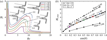
In figure 7, we present the effect of substrate wettability on the wetting length of the upstream wall, keeping the rest of the liquid properties fixed and the inclination angle at
 $a=100^{\circ }$
. It is possible to create substrates with contact angle in the range from
 $5^{\circ }$
to
 $175^{\circ }$
(Duez et al.
Reference Duez, Ybert, Clanet and Bocquet2010). Clearly, the more hydrophilic the substrate, the larger the force applied on the contact point,
 $F_{CL}=\unicode[STIX]{x1D70E}\cos (\unicode[STIX]{x1D703})$
, trying to increase the wetting length. In figure 7(a), we observe that
 $H_{1}$
exhibits the same variation with
 $Re$
as in figure 6, irrespective of the particular value of
 $\unicode[STIX]{x1D703}$
. Moreover
 $H_{1}$
decreases monotonically with increasing
 $\unicode[STIX]{x1D703}$
for the same
 $Re$
. In less hydrophilic substrates, the contact line force decreases and the transition to the inertia–gravity region is less drastic, see figure 7(a), curve (iv). All curves exhibit a hysteresis loop, except for the curve with
 $\unicode[STIX]{x1D703}=80^{\circ }$
. At even slightly higher
 $\unicode[STIX]{x1D703}$
,
 $H_{1}=0$
for
 $Re$
around 1.5 and larger than 10. Finally at
 $\unicode[STIX]{x1D703}\sim 89.5^{\circ }$
(not shown) the maximum wetting length becomes zero for all
 $Re$
, except for
 $Re\approx 0$
where it approaches infinity as expected from (4.2). We present film shapes and streamline patterns at the
 $H_{1}$
-maximum for each
 $\unicode[STIX]{x1D703}$
-curve as insets. They make clear that with increased hydrophilicity not only
 $H_{1}$
, but also
 $H_{2}$
increases and that the minimum in the outer surface is always located around the midplane between the slit walls. For
 $\unicode[STIX]{x1D703}=70^{\circ }$
and more so for
 $\unicode[STIX]{x1D703}=80^{\circ }$
,
 $H_{2}$
decreases so much that the number of ‘Moffatt’ vortices decreases considerably. In fact, Moffatt (Reference Moffatt1964) has shown that, when the two surfaces bounding the corner are flat, no eddy can appear for
 $\unicode[STIX]{x1D703}\geqslant 78.2^{\circ }$
.
(a) The liquid wetting length on the upstream wall versus the Reynolds number for different values of contact angle
 $\unicode[STIX]{x1D703}$
, (b) the maximum penetration of the liquid flow in the transition region as a function of the contact angle, for different
 $Ka$
and at inclination angle
 $a=100^{\circ }$
. Calculations in (b) have been made in increments of
 $5^{\circ }$
. The slopes of the interpolating lines are 2.66 for
 $Ka=5$
, 4.17 for
 $Ka=10$
and 6.05 for
 $Ka=15$
, indicating an almost linear increase with
 $Ka$
.

In figure 7(b) we present the maximum penetration of the liquid at the upstream wall, which occurs at intermediate
 $Re$
, as a function of
 $\cos (\unicode[STIX]{x1D703})$
, which is a measure of the contact line force, for different values of
 $Ka$
. We observe that
 $H_{1,max}$
depends almost linearly on both
 $\cos (\unicode[STIX]{x1D703})$
and
 $Ka$
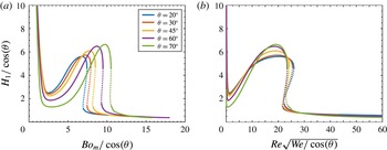
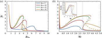
. This observation along with the discussion of figure 6, call for examining whether the critical points in these curves would collapse by appropriately rescaling the axes in figure 7(a). The required different scalings in various parameter ranges to obtain satisfactory approximations of the wetting lengths will be discussed in § 4.1.6.
4.1.3 Effect of
 $Ka$

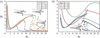
Figure 8 presents the dependence of
 $H_{1}$
on the Reynolds number for different values of the Kapitza number. As the flow rate increases, all liquids exhibit the same pattern of a minimum in
 $H_{1}$
and a hysteresis loop, except for those with the highest viscosity
 $(Ka\leqslant 5)$
, which do not exhibit a hysteresis. In such liquids, although
 $H_{1}$
varies non-monotonically, it remains small for all flow rates. In figure 8(b) we observe that for larger
 $Ka$
the hysteresis does take place in a short range of
 $Re$
. As
 $Ka$
increases, due to the increase of both the capillary force on the inner interface and the force at the contact points
 $(F_{CL}=\unicode[STIX]{x1D70E}\,\cos (\unicode[STIX]{x1D703}))$
or the decrease in liquid viscosity, wetting increases for almost all
 $Re$
. Moreover, the critical Reynolds values of the minimum and the two turning points shift to greater values. At
 $Ka\sim 15.6$
a new solution family appears in the form of an isola and as such it introduces two additional branches of solutions. It is depicted in figure 8(a) in the range
 $13.3<Re<20.3$
, for
 $Ka=16$
. In the upper branch of the isola, the main vortex spans the entire width of the slit and the first Moffatt eddy is visible (shape ii). In the lower branch, the smaller
 $H_{1}$
prevents the main vortex from reaching the upstream wall and a vortex of very small extent appears next to the upstream corner. The outer region penetrates deeper into the slit in comparison to the previous configuration (shape iii). A steady configuration arises at a similar value of
 $Re$
, but in the original branch of solutions (shape i). Here
 $H_{1}$
is much larger, a lip vortex covering the entire upstream wall arises along with the Moffatt eddies and the outer interface exhibits a much deeper minimum.
The liquid wetting length on the upstream wall of the slit for different liquids in terms of
 $Re$
for (a)
 $Ka\leqslant 16$
and (b)
 $Ka\geqslant 18$
, with
 $\unicode[STIX]{x1D703}=60^{\circ }$
and at inclination angle
 $a=100^{\circ }$
.

At
 $Ka\sim 17.95$
the part of the original solution family up to a region between the two limit points merges with the upper branch of the isola and its remaining part merges with the lower branch of the isola via a transcritical bifurcation. The new family structure is given in figure 8(b) for
 $Ka=18$
with curves indicating their stability as inferred from continuity in parameter space from those before the bifurcation. This restructuring forms a new isola starting at
 $Re\sim 14$
and a new branch extending from very small to large
 $Re$
, but with
 $H_{1}$
not approaching zero for the
 $Re$
values examined. The new solution families are populated by liquid arrangements resembling the ones in the corresponding original branches, as expected (Seydel Reference Seydel2010). Interestingly, the new open branch again has two limit points and exhibits a hysteresis loop for
 $18\leqslant Ka\leqslant 30$
, but this hysteresis vanishes for
 $Ka=45$
. As the Kapitza number increases, the wetting length along the upstream wall increases so that the vortex attached to it connects with the first Moffatt vortex and the minimum in the outer interface increases considerably. Shape (i) in figure 8(b) depicts this arrangement just before the two vortices merge into a larger one. As the Kapitza number increases liquid penetration increases and the vortices merge at lower values of the Reynolds number. Moreover, in figure 8(b) we observe that as
 $Ka$
increases the new isola decreases in size and finally at
 $Ka\sim 26$
it vanishes. For even higher
 $Ka$
only the upper branch remains void of hysteresis or other interesting phenomena. The sections of all four families in figure 8(b) decrease linearly with
 $Re$
for
 $Re>18$
, denoting that inertia, which is the dominant force in this regime, tries to dewet the upstream wall.
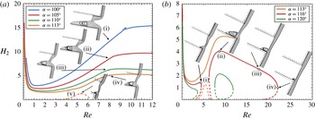
Wetting length on the downstream wall as a function of
 $Re$
for different values of the inclination angle (a)
 $\unicode[STIX]{x1D6FC}=100^{\circ },105^{\circ },110^{\circ },113^{\circ }$
, (b)
 $\unicode[STIX]{x1D6FC}=113^{\circ },116^{\circ },120^{\circ }$
for a liquid with
 $Ka=10$
at contact angle
 $\unicode[STIX]{x1D703}=60^{\circ }$
.

4.1.4 Effect of inclination angle
In figure 9 we present the effect of the orientation of the substrate wall on the wetting length at the downstream wall for different
 $Re$
. The inclination angle affects not only the gravity component driving the flow, but also its secondary component, which opposes liquid entering the slit. By increasing
 $\unicode[STIX]{x1D6FC}$
, always above
 $90^{\circ }$
, the
 $y$
-component of gravity increases, decreasing monotonically
 $H_{2}$
, as shown in figure 9(a).
 $H_{1}$
decreases also remaining always smaller than
 $H_{2}$
, as observed in the shapes (i)–(iv). As the inclination angle increases the space available for the Moffatt eddies decreases and the minimum in the outer interface decreases and translates downstream for the same
 $Re$
. For values above
 $\unicode[STIX]{x1D6FC}\sim 102^{\circ }$
this gravity component is large enough so that liquid arrangements do not exhibit hysteresis making the transition to the inertia–gravity region smooth. For
 $\unicode[STIX]{x1D6FC}=113^{\circ }$
in addition to the original family of solutions, a second family is observed, albeit for a very limited range of
 $Re$
, where even
 $H_{2}$
is greatly diminished; see shape (v) in figure 9(a). At this point the stability of this new family cannot be inferred and will be deduced subsequently.
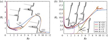
Wetting lengths (a)
 $H_{1}$
and (b)
 $H_{2}$
as a function of
 $Re$
for different values of the width of the slit
 $W=5,\;8,\;9,\;9.1,\;12,\;18$
, for substrate inclination
 $\unicode[STIX]{x1D6FC}=110^{\circ }$
, for a liquid with
 $Ka=10$
at contact angle
 $\unicode[STIX]{x1D703}=60^{\circ }$
.

Examining closer the dual solution families with
 $\unicode[STIX]{x1D6FC}\geqslant 113^{\circ }$
in figure 9(b), we find that the distance between them decreases and finally for
 $\unicode[STIX]{x1D6FC}\sim 114^{\circ }$
they intersect each other forming a transcritical bifurcation (Seydel Reference Seydel2010). Subsequently, two new solution families re-emerge, in a way that for
 $\unicode[STIX]{x1D6FC}=116^{\circ }$
the first one exists for
 $Re<4.5$
and the second one for
 $6<Re<22$
. No other solutions were found for the same inclination angle. The first solution family exhibits a limit point and then
 $H_{2}$
decreases monotonically to zero as
 $Re$
decreases. This turning point occurs for a
 $Re$
larger than that for which the minimum in figure 6 (shape ii) or when liquid inertia has started to play a role. The second family has the shape of an isola. At all solutions on the isola,
 $H_{1}$
remains almost constant and very small
 ${\sim}0.05$
, while
 $H_{2}$
varies up to 4 in the upper branch and down to zero in the lower branch. It is the first time that such liquid arrangements have appeared with almost invisible
 $H_{1}$
and even more so in the lower isola branch where
 $H_{2}>H_{1}$
. For
 $Re>22$
at
 $\unicode[STIX]{x1D6FC}=116^{\circ }$
, only the Cassie–Baxter state seems to occur, with both contact points pinned at the edge of the slit. As the inclination angle increases the isola shrinks very fast, see figure 9(b) for
 $\unicode[STIX]{x1D6FC}=120^{\circ }$
, and for
 $\unicode[STIX]{x1D6FC}\sim 121.6^{\circ }$
this solution family vanishes, while only the first solution family at low values of
 $Re$
remains. The increased gravity component opposing liquid from entering the slit leads to the development of solution branches that turn both
 $H_{1}$
and
 $H_{2}$
toward zero values. As observed in figure 9(b) (shape i) the solution near the turning point reveals that the effect of gravity is to pull most of the liquid outside the slit. As the inclination angle increases the
 $y$
-component of the gravity increases further and the turning point shifts to even lower values of
 $Re$
, see figure 9(b) for
 $\unicode[STIX]{x1D6FC}=120^{\circ }$
. At
 $Re$
for which no similar steady solutions could be found it is possible that perfect Cassie–Baxter shapes arise or the liquid starts dripping as soon as it arrives at the upstream corner of the slit.
The new connectivity of the solution families in figure 9(b) can be used to infer their stability (Iooss & Joseph Reference Iooss and Joseph1990; Seydel Reference Seydel2010). Given that the original branch with
 $Re\rightarrow 0$
is stable, it is deduced that the branch after the limit point with
 $\unicode[STIX]{x1D6FC}=116^{\circ }$
is unstable as indicated by the dashed line. Proceeding in this way, the stability of all the remaining solution branches is deduced and shown in figure 9.
4.1.5 Effect of slit width
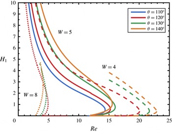
Figure 10 presents the effect of increasing the width of the slit from
 $W=5$
, which is the value we used so far. For the same
 $Re$
, the variation of
 $H_{1}$
, when
 $W$
increases from 5 to 8 and even to 9 is rather small as can be seen in figure 10(a), because the lines overlap for the most part, while the variation of the consistently much larger
 $H_{2}$
is somewhat more affected. The usual local minimum followed by the hysteresis loop can be seen in these three cases. Some typical film shapes for
 $W=8$
are given as insets in figure 10(a). Two Moffatt eddies can be seen for
 $Re\sim 4.5$
in spite of the small value of
 $H_{2}$
. Both penetration distances increase at
 $Re\sim 8.5$
, but only one eddy can be seen because of the reduced intensity of the others.
At
 $Re\sim 10$
, the increased inertia assists in dewetting the upstream wall and the intensified ‘splashing’ of the liquid on the downstream slit wall increases
 $H_{2}$
. Observing closely figure 10(b), we find that for
 $W=8$
and 9 new solution families arise for
 $3.5<Re<5.5$
with smaller values of
 $H_{2}$
compared to the original families. For
 $Re\sim 4.5$
the two families with
 $W=9$
have approached each other and a very small increase of
 $W$
to 9.1 induces rearrangement of the families similar to the one we observed in figure 9(b). This creates two new families with limit points at
 $Re\sim 4.2$
and 4.7. The first family evolves towards smaller
 $Re$
and can be seen for
 $W=12$
and 18, while the second one evolves towards larger
 $Re$
and quickly relocates to much higher
 $Re$
, so it is not depicted in figure 10(b). In the same figure we give as insets film shapes above the slit, when
 $H_{2}$
attains a local maximum. As
 $W$
increases the local maximum occurs at smaller
 $Re$
value and the film becomes progressively thinner. It is possible that for so large slit widths the film will break as observed in our transient simulations (Lampropoulos et al.
Reference Lampropoulos, Dimakopoulos and Tsamopoulos2016). On the contrary, its segments closer to the two slit walls do not vary considerably. Curves corresponding to the new families with small
 $H_{2}$
cannot be seen in figure 10(a) and after the change in the connectivity of families only the branches for smaller
 $Re$
can be identified.
4.1.6 Scaling laws
Bontozoglou & Serifi (Reference Bontozoglou and Serifi2008) have studied film flow over a trench of finite depth, under the assumption that the liquid completely fills the trench. They have concluded that, depending on the forces dominating the flow, its patterns can be split into 3 types: patterns determined by the ‘capillary–gravity’ balance, for low values of
 $Re$
, those determined by the ‘inertia–gravity’ balance for high values of
 $Re$
and those in a transition region in between, where capillarity competes with inertia and gravity. We will extend their ideas and those reported previously by Kalliadasis et al. (Reference Kalliadasis, Bielarz and Homsy2000) and Mazouchi & Homsy (Reference Mazouchi and Homsy2001) in order to investigate the interplay of the forces acting in this quite more complicated problem. First we will examine the dependence of
 $H_{1}$
on these forces for different values of
 $Re$
. Subsequently we will examine the dependence of
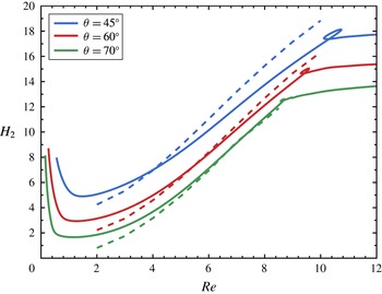
 $H_{2}$
on the same parameters.
In the capillary–gravity regime, as already discussed in relation to figures 5 and 6, the variation of
 $H_{1}$
for low
 $Re$
(up to its minimum value) is determined by
 $Bo_{m}$
. It is anticipated, therefore, that by plotting
 $H_{1}$
versus
 $Bo_{m}$
these minima will arise for the same value of
 $Bo_{m}$
. We will now turn our attention in the regime where the effect of inertia becomes important.
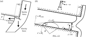
(a) Sketch that presents the part of the film near the upstream corner including the upstream wetting length. We indicate the main applied forces and the extent over which the capillary force is effective resulting in a curved inner interface denoted by
 $L^{\ast }$
. (b) Sketch that defines the scales for the part of the film near the downstream wall. The origin of the local coordinates
 $(x^{\prime },\;y^{\prime })$
is set at the entrance of the film that wets the downstream wall while the film height in that region is denoted by
 $L^{\prime }$
.

In order to assist in the examination of the dominant force balance, we have prepared figure 11. First, we will focus our attention in the part of the inner interface close to the upstream wall (see figure 11
a). For moderate to high values of the Reynolds number, the deformed interface is characterized by the length
 $L^{\ast }$
, beyond which the liquid does not feel the presence of the wall and becomes flat. In other words,
 $L^{\ast }$
is the length scale of the capillary features in the streamwise direction. The combined effect of inertia and gravity act as to drive the liquid in the streamwise direction tending to decrease
 $H_{1}^{\ast }$
. This action is opposed by capillarity which drives liquid along the upstream wall and, thus, the following simplified momentum balance holds:
 $$\begin{eqnarray}\unicode[STIX]{x1D70C}g+\frac{\unicode[STIX]{x1D70C}U^{\ast 2}}{L^{\ast }}\approx \frac{\unicode[STIX]{x1D70E}H_{1}^{\ast }}{L^{\ast 3}},\end{eqnarray}$$
where
 $\unicode[STIX]{x1D70C}g$
is the gravity force, the second term in the left-hand side characterizes the inertia force and, finally, the capillary pressure has been approximated as
 $p^{\ast }\approx \unicode[STIX]{x1D70E}\;\unicode[STIX]{x2202}^{2}h^{\ast }/\unicode[STIX]{x2202}x^{\ast 2}\Rightarrow \unicode[STIX]{x2202}p^{\ast }/\unicode[STIX]{x2202}x^{\ast }\approx \unicode[STIX]{x1D70E}\;\unicode[STIX]{x2202}^{3}h^{\ast }/\unicode[STIX]{x2202}x^{\ast 3}\sim \unicode[STIX]{x1D70E}\,H_{1}^{\ast }/L^{\ast 3}$
; the viscous effects are taken implicitly into account through the definition of the characteristic velocity based on the Nusselt film flow. The key in this expression is the determination of
 $H_{1}^{\ast }$
, which can also be considered as a measure of the bending of the inner interface by surface tension forces, in terms of the Nusselt thickness
 $H^{\ast }$
. First it should be noted that the wetting length
 $H_{1}^{\ast }$
should depend on the level of the force applied on the contact point,
 $F_{CL}=\unicode[STIX]{x1D70E}\cos (\unicode[STIX]{x1D703})$
. Hence, it is reasonable to expect that
 $H_{1}^{\ast }$
should be also proportional to
 $\cos \unicode[STIX]{x1D703}$
and
 $Ka$
, which is a measure of the surface tension with respect to the viscous forces. This latter dependence of
 $H_{1}^{\ast }$
on the wettability and
 $Ka$
has also been observed in figure 7(b). Therefore for the purpose of the scaling arguments, we will assume that
 $H_{1}^{\ast }\approx H^{\ast }Ka\;\cos \unicode[STIX]{x1D703}$
is the proper scale for
 $H_{1}^{\ast }$
. Introducing this expression in (4.4) we obtain:
 $$\begin{eqnarray}\unicode[STIX]{x1D70C}g+\frac{\unicode[STIX]{x1D70C}U^{\ast 2}}{L^{\ast }}\approx \frac{\unicode[STIX]{x1D70E}H^{\ast }}{L^{\ast 3}}Ka\cos (\unicode[STIX]{x1D703}).\end{eqnarray}$$
In the high
 $Re$
regime, balancing inertia to capillarity and neglecting for now the effect of gravity we obtain:
 $$\begin{eqnarray}L^{\ast }\approx \frac{\cos ^{1/2}(\unicode[STIX]{x1D703})Ka^{1/2}}{Re^{1/2}Ca^{1/2}}H^{\ast }.\end{eqnarray}$$
When the transition from the capillary–gravity region to the inertia–gravity region has taken place, all three terms in (4.5) must balance each other yielding:
 $$\begin{eqnarray}Re\frac{We^{1/2}}{\cos ^{1/2}(\unicode[STIX]{x1D703})}\approx St/Ka^{1/2}.\end{eqnarray}$$
This expression indicates that, for constant inclination angle and the same liquid (i.e.
 $St,\;Ka$
constant), its left-hand side must remain constant. On the other hand, if
 $Ka$
varies and the contact angle remains constant, the following expression must remain constant:
 $$\begin{eqnarray}Re^{1/6}We=\text{const}.\Rightarrow We\approx \text{const}.\end{eqnarray}$$
To check how our scaling analysis compares against our numerical results we show in figure 12(a,b) the dependence of
 $H_{1}/\text{cos}(\unicode[STIX]{x1D703})$
either on
 $Bo_{m}/\text{cos}(\unicode[STIX]{x1D703})$
or on
 $Re\sqrt{We/\text{cos}(\unicode[STIX]{x1D703})}$
, respectively. Indeed this figure demonstrates that the minimum of all curves occurring for low
 $Re$
arises in a very short range
 $2.50\leqslant Bo_{m}/\text{cos}(\unicode[STIX]{x1D703})\leqslant 2.75$
and that the two limit points at high
 $Re$
arise also in a very short range
 $21.5\leqslant Re\sqrt{We/\text{cos}(\unicode[STIX]{x1D703})}\leqslant 23$
. Clearly these critical points vary in a much wider range of
 $Re$
in figures 6 and 7. Having scaled the effect of wettability, this observation verifies again that at the local minimum of
 $H_{1}^{\ast }$
a balance between capillary and gravity forces prevails and that hysteresis arises because of an interplay between inertia and gravity forces. It should be noted that since
 $Bo_{m}=W\cdot Ca\cdot St$
and the Stokes number is constant in figure 12(a),
 $Ca$
also varies in a short range.
The rescaled liquid wetting length on the upstream wall,
 $H_{1}/\text{cos}(\unicode[STIX]{x1D703})$
, versus (a)
 $Bo_{m}/\text{cos}(\unicode[STIX]{x1D703})$
and (b)
 $Re\sqrt{We/\text{cos}(\unicode[STIX]{x1D703})}$
for different values of contact angle
 $\unicode[STIX]{x1D703}$
, while
 $Ka=10$
and
 $a=100^{\circ }$
.

To examine if the scaling arguments presented above are valid for different materials, we plot
 $H_{1}$
as a function of either
 $Bo_{m}$
or
 $We$
for different values of
 $Ka$
, in figure 13. In figure 13(a) we observe that all families exhibiting a sharp minimum for small
 $Re\,(Ka=10,15,16)$
, it arises for almost the same Bond number
 $Bo_{m}\sim 1.25$
or
 $Ca\sim 0.09$
. Beyond this value, liquid inertia starts playing a more significant role in the force balance. Then, figure 13(b) demonstrates that the second turning point arises at constant Weber number
 $We\sim 2.8$
. In the inset of figure 13(b) we rescale the
 $y$
-axis as suggested earlier and we observe a gratifying collapse of their maxima. This collapse of the critical points and of the maxima in these families should be compared with the wide range of
 $Re$
for which they arise in figure 8(a).
Next we turn our attention in the part of the inner interface that wets the downstream wall (see figure 11
b) and perform an approximate analysis to determine the dependence of
 $H_{2}^{\ast }$
on the various problem parameters. For the purposes of this analysis, we will consider the indicated set of local coordinates
 $(x^{\prime },y^{\prime })$
, the origin of which lies at the position of maximum height of the film that wets the downstream wall and denote the new dimensional variables by ‘
 $^{\prime }$
’. We also denote the film height in that region by
 $L^{\prime }$
, while the distance to the contact line is denoted by
 $H_{2}^{\prime }$
. It can be seen in figure 6 that for a wide range of
 $Re$
values the film that wets the downstream wall can be largely divided into two different regions. One region near the contact line where the shape of the interface is highly curved and a second region far from the contact line where the interface can be considered as nearly flat. In the contact line region (
 $H_{2}^{\prime }\geqslant x^{\prime }\geqslant X_{m}^{\prime }$
) the surface tension effects become dominant and thus it is reasonable to assume that the shape of the interface will acquire the shape of spherical cap with radius
 $R^{\prime }$
and centre
 $(x_{o}^{\prime },y_{o}^{\prime })=(H_{2}^{\prime }-R^{\prime }\sin \unicode[STIX]{x1D703}^{\prime },-R^{\prime }\cos \unicode[STIX]{x1D703}^{\prime })$
. Thus we assume that the interface in this region can be described by the following equation
 $$\begin{eqnarray}y^{\prime }=\sqrt{R^{\prime 2}-(x^{\prime }-H_{2}^{\prime }+R^{\prime }\sin \unicode[STIX]{x1D703}^{\prime })^{2}}-R^{\prime }\cos \unicode[STIX]{x1D703}^{\prime }.\end{eqnarray}$$
The liquid wetting length on the upstream wall in terms of (a)
 $Bo_{m}$
and (b)
 $We$
, for different liquids using a liquid with
 $\unicode[STIX]{x1D703}=60^{\circ }$
and at inclination angle
 $a=100^{\circ }$
.

Far from the contact line (
 $0\leqslant x^{\prime }\leqslant X_{m}^{\prime }$
) the interface can be considered nearly flat and therefore it can be described by
 $$\begin{eqnarray}y^{\prime }=-\frac{L^{\prime }}{H_{2,max}^{\prime }}x^{\prime }+L^{\prime }.\end{eqnarray}$$
It can be seen in figures 6 and 7 that
 $L^{\prime }$
is approximately constant for a wide range of
 $Re$
and thus for our analysis we will assume that
 $L^{\prime }\approx W^{\ast }/2$
.
 $H_{2,max}^{\prime }$
, on the other hand, denotes the theoretical limit that the liquid would reach in the absence of contact line effects, e.g. in the case of a prewetted solid surface (
 $\unicode[STIX]{x1D703}^{\prime }=0$
), due to the effect of inertia that would be counterbalanced by the effect of gravity. It is possible to provide an estimate for
 $H_{2,max}^{\prime }$
by considering that the hydrostatic pressure at
 $x^{\prime }=0$
should be balanced by the dynamic pressure in that region which leads to the following pressure balance
 $$\begin{eqnarray}\frac{\unicode[STIX]{x1D70C}U^{\ast 2}}{2}\approx \frac{\unicode[STIX]{x1D70C}g_{x^{\prime }}H_{2,max}^{\prime }}{2}=-\frac{\unicode[STIX]{x1D70C}gH_{2,max}^{\prime }}{2}\cos a.\end{eqnarray}$$
For the estimation of the dynamic pressure we assume that the average velocity in the narrowest part of the film, i.e. the velocity at which the film impacts the downstream wall, is approximately equal to the Nusselt velocity. This assumption is justified by the fact that the cross-section of the neck can be considered approximately equal to the Nusselt film height (see figures 6 and 7). From (4.11) we derive the following expression for
 $H_{2,max}^{\prime }$
 $$\begin{eqnarray}H_{2,max}^{\prime }=-\frac{Re}{St\cos a}H^{\ast }.\end{eqnarray}$$
Due to the fact, however, that the solid is partially wetted, the contact line actually equilibrates at
 $H_{2}^{\prime }<H_{2,max}^{\prime }$
.
 $H_{2}^{\prime }$
can be evaluated by realizing that the capillary pressure due to the curved liquid–air interface near the contact line should compensate for the reduced hydrostatic pressure due to the missing liquid beyond the contact line leading to the following pressure balance
 $$\begin{eqnarray}\frac{\unicode[STIX]{x1D70E}}{R^{\prime }}\approx -\frac{\unicode[STIX]{x1D70C}g\left(H_{2,max}^{\prime }-H_{2}^{\prime }\right)}{2}\cos a,\end{eqnarray}$$
and thus
 $$\begin{eqnarray}H_{2}^{\prime }\approx H_{2,max}^{\prime }+\frac{2}{R^{\prime }}\frac{H^{\ast 2}}{Bo\cos a}.\end{eqnarray}$$
The slopes and height of the interface should match at the boundary of the two regimes, i.e. at
 $x^{\prime }=X_{m}^{\prime }$
, and from this matching we can evaluate the radius of curvature,
 $R^{\prime }$
, as follows
 $$\begin{eqnarray}R^{\prime }=\frac{L^{\prime }(H_{2,max}^{\prime }-H_{2}^{\prime })}{\sqrt{{H_{2,max}^{\prime }}^{2}+L^{\prime 2}}-L^{\prime }\sin \unicode[STIX]{x1D703}^{\prime }-H_{2,max}^{\prime }\cos \unicode[STIX]{x1D703}^{\prime }}.\end{eqnarray}$$
By combing (4.14) and (4.15) we derive the following analytical expressions for
 $R^{\prime }$
 $$\begin{eqnarray}R^{\prime }=\left[\frac{-2L^{\prime }}{Bo\cos a\left(\sqrt{{H_{2,max}^{\prime }}^{2}+L^{\prime 2}}-L^{\prime }\sin \unicode[STIX]{x1D703}^{\prime }-H_{2,max}^{\prime }\cos \unicode[STIX]{x1D703}^{\prime }\right)}\right]^{1/2}H^{\ast },\end{eqnarray}$$
which can be introduced in (4.14) to compute
 $H_{2}^{\prime }$
. Subsequently
 $H_{2}^{\ast }$
can be evaluated by noting that the entrance of the film that wets the downstream wall is located approximately at the same position where the contact line in the upstream wall resides (see figure 6) and thus
 $H_{2}^{\ast }\approx H_{1}^{\ast }+H_{2}^{\prime }$
.
We plot the latter semi-analytical expression in figure 14 and compare it against our numerical computations for three different values of the contact angle. As it is shown, our scaling analysis can capture very well the overall dependence of the wetting length of the downstream wall for a wide range of parameter values. The agreement is indeed remarkable for the highest value of the contact angle and somewhat deteriorates with increasing hydrophilicity of the solid surface. The latter could be attributed to some extent to the fact that the neck cross-section of the film that impacts the downstream wall becomes thicker with decreasing
 $\unicode[STIX]{x1D703}$
(see figure 7) which would result in deceleration of the flow, i.e. lower velocity than the Nusselt velocity. This effect has not been accounted for in (4.11) and may lead to an overestimation of
 $H_{2,max}^{\prime }$
for lower values of
 $\unicode[STIX]{x1D703}$
.
Wetting length of the downstream wall
 $H_{2}$
, as a function of the Reynolds number for different values of the contact angle
 $\unicode[STIX]{x1D703}$
for a liquid with
 $Ka=10$
and at inclination angle
 $a=100^{\circ }$
. The solid and dashed lines present our numerical calculations and the results from scaling analysis, respectively.

4.2 Hydrophobic surfaces
4.2.1 General pattern
In figure 15 we present the wetting lengths for a liquid having
 $Ka=$
100 on a hydrophobic surface, which can occur only for inclination angles less than
 $90^{\circ }$
, otherwise no slit wetting is possible, as explained previously. Here the direction of gravity and capillarity is inverted, the
 $y$
-component of gravity pushes the liquid inwards, but capillarity and hydrophobicity oppose it, see (4.2). The flow kinematics are similar to the hydrophilic case, except for the significant difference that with a contact angle above
 $90^{\circ }$
, the formation of Moffatt eddies is disallowed (Moffatt Reference Moffatt1964). Indeed in the liquid inside the slit only a single vortex appears, if any, which is not of the Moffatt type. As the flow rate and
 $Re$
tend to zero, this vortex increases in size, but decreases in strength, leaving capillarity as the only remaining force to maintain the liquid from leaking. Hence, the velocity pointing outward from the slit in the upper contact point diminishes the tendency of the wetting length to increase; compare shapes (i)–(iii) in figure 15. This mechanism is similar to the one producing the teapot effect as
 $Re$
decreases (Kistler & Scriven Reference Kistler and Scriven1994). In contrast to figure 6, here no local minimum arises in either
 $H_{1}$
or
 $H_{2}$
curve, but both decrease monotonically until the first limit point. The reason for this major difference is that here the increase in
 $Re$
and the flow rate, although it increases the approach velocity to the downstream slit wall, it cannot spread the liquid there because of its hydrophobic character. Instead, the increased velocity in the vicinity of the contact point A tends to pull the liquid out of the slit. This increased resistance to liquid penetration necessitates the increase in the capillary rise in (point E in figure 1) of the outer interface (compare shapes i–iv before the slit entrance) in order to counter-balance it. Because a fluid particle ejected from the plane in the outer region lands further away from the upstream corner as
 $Re$
increases, the inner free surface is at an angle with respect to the outer one and the vortex assumes a nearly triangular shape, see figure 15(iii–iv).
Dependence of the wetting lengths
 $H_{1}$
(black line, points marked
 $\bullet$
) and
 $H_{2}$
(green line, points marked
 $\circ$
) on
 $Re$
at contact angles
 $\unicode[STIX]{x1D703}=120^{\circ }$
, for a liquid with
 $Ka=100$
at inclination angle
 $a=60^{\circ }$
and slit width
 $W=5$
. The continuous and discontinuous green lines have been obtained by parameter continuation allowing
 $H_{1}$
to be finite when possible or zero, respectively. The same curve types are used in similar figures that follow. The arrows indicate the ‘hysteresis jumps’ in
 $H_{1}$
, when
 $Re$
exceeds the respective values at the two limit points forming the hysteresis loop. Film shapes for
 $Re$
less than that in the vertical dotted line have an inner interface which deep inside the trench intersects the upstream wall. Solutions to the left of the one indicated with the empty square form contact angles with the upstream wall, which do not satisfy inequality (4.17).

The previous pattern cannot continue, because the decreasing
 $H_{1}$
forces the vortex to detach from the upstream wall. This brings about a limit point at
 $Re$
slightly above 15.2, see shape (iv) in figure 15. Interestingly, at this point
 $Bo^{\ast }=$
0.6, indicating that although the gravitational force has been increasing along with
 $Re$
, it has not yet balanced capillarity. As
 $Re$
starts to decrease after the limit point, recirculation is pushed away from the upstream wall. Its approach to the downstream wall forces contact point B to advance along the downstream wall. These two effects result in a decrease in
 $H_{1}$
and a small increase in
 $H_{2}$
, a trend which continues until
 $Re\sim 12.6$
, typical is the shape (v) in figure 15. Shortly after this value of Reynolds the upstream wall is completely dewetted and contact point ‘A’ gets pinned at the upstream corner. Now it is not necessary for the contact angle with the upstream wall to equal
 $120^{\circ }$
, but it is free to adjust to the flow kinematics and dynamics. This signals a second turning point, with
 $Re$
increasing again. In this new branch, shape (vi) in figure 15 indicates that in fact the film seems to be ejected straight from the plane wall, as its inner interface follows a straight path and the capillary rise in its outer interface decreases. The latter effect decreases the capillary pressure from the outer interface, which becomes insufficient to push the fluid to the downstream wall. Dewetting of the downstream wall starts, while the recirculation close to contact line B vanishes; see shape (vi) in figure 15. Further increase of
 $Re$
leads to complete dewetting of the slit; see shape (vii) in figure 15. Finally at
 $Re\sim 20$
an ideal Cassie–Baxter state appears. This family of solutions is depicted with continuous lines in figure 15.
Considering the stability of the film shapes just presented, one could argue that, when
 $Re$
is small enough, the inner interface has a constant curvature. Then the capillary force that holds the liquid column is constant, but gravity varies with the penetration depth. If the interface moves slightly down, gravity prevails, more liquid moves towards the slit and the flowing film raptures. In the opposite direction, if the interface moves slightly up, capillarity wins and the liquid is ejected out of the slit. Therefore these equilibrium shapes are unstable. However, the transition from shapes of rather constant curvature in the inner interface to shapes with highly variable curvature as
 $Re$
increases is smooth; see figure 15. This transition seems to occur between shapes (ii) and (iii) and makes it unclear when the constant curvature assumption is a safe one. To remedy this problem we decided to retain all the previously computed shapes without indicating their stability along each family and we proceeded to add to this family a second family in which the contact point in the upstream wall is pinned at the respective corner of the substrate and the corresponding contact angle may adjust freely to almost any value, while the position of the contact point ‘B’ is still determined by fixing the contact angle there. It seems that this new family extends from very low
 $Re$
values to the second limit point of the first family. It is depicted by the dashed line in figure 15 and a typical film arrangement is inset (viii). Here the inner surface closer to the upstream corner is nearly flat, but bends sharply as it approaches the downstream wall to adjust its contact angle there. For values of
 $Re$
larger than this limit point the two families merge, because both are populated with film shapes in which
 $H_{1}=0$
and
 $H_{2}$
is adjusted so that the contact line condition is satisfied.
In the new solution family we observe that below a specific value of
 $Re$
which is
 ${\sim}5$
, the calculated width of the inner interface deep inside the trench becomes larger than the width of the trench. Then, the inner interface intersects the upstream wall for a second time. This corresponds to the case depicted in figure 2(f) in Kistler & Scriven (Reference Kistler and Scriven1994). We considered such shapes to be beyond the scope of the present analysis and terminated the respective family at that
 $Re$
value, as indicated by the vertical dotted line. Moreover, we have calculated the angle that the inner interface forms with the upstream wall at the corner. We found that the angle varies from
 $260^{\circ }$
at
 $Re=3$
to
 $210^{\circ }$
in a region close to the second turning point to
 $185^{\circ }$
at
 $Re=20$
. Kistler & Scriven (Reference Kistler and Scriven1994) refer to the Gibbs (Reference Gibbs1906) inequality that describes with simple geometric conditions whether a pinned point will be detached or not. They noted that, if
 $\unicode[STIX]{x1D6FE}$
is the angle of the substrate (in our case
 $\unicode[STIX]{x1D6FE}=90^{\circ }$
), the contact point remains pinned at the corner, if the calculated angle
 $\unicode[STIX]{x1D703}_{p}$
follows the inequality:
 $$\begin{eqnarray}\unicode[STIX]{x1D703}_{p}<\unicode[STIX]{x1D703}+\unicode[STIX]{x1D6FE},\end{eqnarray}$$
where
 $\unicode[STIX]{x1D703}$
is the wettability of the substrate. In the new family of shapes, expression (4.17) holds for
 $Re>12$
, which is a region a little to the left of the second turning point. The discriminating point is indicated by an ‘open square’. Then, solutions with fixed contact point at the upstream corner with
 $Re\leqslant 12$
do not obey it, indicating that wetting of the upstream wall is preferable. This occurs, even for
 $Re$
values larger than those for which the inner interface intersects twice the upstream wall. We could not find another family of static solutions with partial wetting for low values of Reynolds, except of course, for the ideal Cassie–Baxter state with both contact points pinned at the corners of the slit, as long as inequality (4.17) is satisfied. The stability of all three families, when they arise, must be determined by a linear stability analysis or transient simulations. Then, it will become clear which family exists for each
 $Re$
.
4.2.2 Effect of
$Ka$

In figure 16 we present the two wetting lengths in terms of the Reynolds number for different liquids. The previously examined case is included in figure 16(a). In figure 16(a), the new base solution cannot be identified here because in it
 $H_{1}=0$
. On the contrary in figure 16(b), we present both the original (with continuous curves) and the new (with dashed curves) family. In figure 16 along a vertical line with, say
 $Re=10$
, increasing
 $Ka$
requires decrease in the flow rate, which, in turn, decreases liquid recirculation inside the slit and, because of this, it increases the wetting length. In effect the change in the flow kinematics with increasing
 $Ka$
is not different from what takes place as
 $Re$
decreases along a curve with constant
 $Ka$
. The shapes of all curves in figure 16(a) follow the same pattern: a monotonic, sharp decrease of
 $H_{1}$
as
 $Re$
increases until the first limit point, followed by a second limit point leading to the final branch with
 $H_{1}=0$
for all larger
 $Re$
, i.e. inertial hysteresis takes place prior to complete dewetting of both slip wall in all liquids shown in this figure.
(a)
 $H_{1}$
, (b)
 $H_{2}$
versus
 $Re$
for different liquids with
 $Ka=40$
, 80, 100, 200, while
 $\unicode[STIX]{x1D703}=120^{\circ }$
and at inclination angle
 $a=60^{\circ }$
. Solutions to the left of the ones indicated with the empty squares form contact angles with the upstream wall, which do not satisfy inequality (4.17).

For lower
 $Ka$
the hysteresis occurs at smaller Re and its successive limit points are closer together in terms of their Re. For example, they are at
 $Re=4.48$
and 4.15 for the liquid with
 $Ka=40$
; and at
 $Re=30.80$
and 24.10 for
 $Ka=200$
. For the latter value of
 $Ka$
, the film is quite distorted, especially in its outer surface, where the deeper minimum is preceded by standing capillary waves, see inset (i–ii) in figure 16(a). Although the value of
 $Re$
at the turning point is affected drastically by changing
 $Ka$
, we will see below that this is not the case when the dependence of these families on the Bond number or the Weber number is examined. Finally, the new solution family is presented in figure 16(b) (dashed lines). For
 $Ka=200$
, for instance, this family follows the same pattern discussed in figure 15. In the insets (iii–iv) we observe the transition of the solution curve from partial wetting of the downstream wall to almost non-wetting. The contact angle in these insets at the pinned contact point has been calculated as
 $230^{\circ }$
and
 $187^{\circ }$
, respectively. The ‘open squares’ indicate the
 $Re$
values below which the calculated angle at the pinned contact point is below to
 $210^{\circ }$
(
 $=90^{\circ }+120^{\circ }$
). Therefore, inset (iii) is an acceptable solution because the inner interface lies inside the side walls of the slit, but not acceptable because the contact angle does not satisfy inequality (4.17). In other words, for this
 $Re$
, the contact point on the upstream wall should be de-pinned and wetting of the upstream wall should be allowed. This would lead to the steady solution in the other family indicated by the continuous line and the shape is given as inset (i) in figure 16(a). On the contrary, inset (iv) is an acceptable solution.
At
 $Ka=310$
, a new solution family in the form of an isola is observed close to the base solution. Its size rapidly increases with
 $Ka$
. In figure 17(a) for
 $Ka=350$
, we present the base solution family and the isola being very close to each other. They merge at
 $Ka=362$
, through a transcritical bifurcation (Seydel Reference Seydel2010), and the new type of solution family is abruptly extended to higher
 $Re$
, where it exhibits an increase in the velocity, up to the new limit point. In shapes (i)–(iii) of figure 17(a) we present film shapes and streamlines for
 $Ka=450$
. They carry the properties of either the base solution family or the isola.
(a)
 $H_{1}$
, (b)
 $H_{2}$
versus
 $Re$
for different liquids with
 $Ka=200$
, 300, 350, 450, while
 $\unicode[STIX]{x1D703}=120^{\circ }$
and inclination angle
 $a=60^{\circ }$
. Solutions to the left of the ones indicated with the empty squares form contact angles with the upstream wall, which do not satisfy inequality (4.17).

The wetting length is large enough and the recirculation strong enough that in shape (i) of figure 17(a) we can observe even a second vortex near the downstream contact point. Along this family, as
 $Re$
increases, the recirculation inside the slit shrinks, as usual. An abrupt change in slope is seen at
 $Re\sim 52$
(shape ii), reminding us the merging of the two solution families. Its outer interface has characteristics similar to those of shape (ii) in figure 17(a). For higher values of
 $Re$
, the film and flow patterns resemble the corresponding ones of the shapes in the former isola. The solution patterns follow the ballistic-type effect, as we have already discussed. The magnitude of
 $Re$
determines the distance the fluid particle can travel before it lands somewhere between the slit walls. At low
 $Re$
the fluid particle lands closer to the step-in edge of the slit, while as
 $Re$
increases, the ballistic effect shifts the fluid particle closer to the middle of the slit, while the existence of high pressure at the downstream wall pushes the fluid particles outside the slit, compare shapes (ii)–(iii) in figure 17(a). Furthermore, we observe that the wetting of the downstream wall in the new steady-state branch increases as Kapitza increases in figure 17(b). The curves tend to be more vertical with increasing
 $Ka$
, while the ‘squares’ pinpoint the position in which the contact angle is equal to
 $210^{\circ }$
. With further increasing the Reynolds number the two families merge after the second turning approaching the ideal Cassie state (see shapes (vi)–(viii)).
As we already mentioned for smaller
 $Ka$
the hydrophilic wetting family (figure 13) can be split into three regions depending on the dominant force balance in each region. For
 $Bo_{m}\geqslant 1.25$
the capillary–gravity region exists, while for
 $We>2.8$
the inertia–gravity region exists initiated by the hysteresis loop and between them the transition region exists. In hydrophobic surfaces however, this pattern is not followed. No minimum in the wetting lengths appears before the first turning point, which occurs at
 $Bo_{m}\sim 0.6$
and the capillary rise at point E (in figure 1) is prominent at intermediate values of
 $Re$
. Comparing the wetting lengths in figures 6 and 15 and in spite of the somewhat different
 $Ka$
, we can generally state that in hydrophobic surfaces, they are larger for
 $Re<6$
, but quite smaller for
 $Re>6$
. Moreover, examining the wetting length dependence on
 $Re$
in figure 16, we find that it does not provide a characteristic value as to where the hysteresis loop arises. On the contrary, if we examine their dependence on
 $Bo_{m}$
or
 $We$
things change dramatically, as can be seen in figure 18. In figure 18(a) we observe that the first limit point occurs in the range
 $0.625<Bo_{m}<0.675$
, when
 $Ka\geqslant 200$
. Indicatively we also give the corresponding family for
 $Ka=300$
to demonstrate that for higher
 $Ka$
the critical
 $Bo_{m}\sim 0.585$
and the previous pattern is not followed. Instead, figure 18(b) shows that the first limit point arises for
 $1<We<1.05$
, when
 $Ka\geqslant 300$
, but for much smaller and widely varying
 $We$
when
 $Ka<300$
. When the isola appears and even merges with the original family for
 $Ka=362$
the limit point abruptly moves to much larger values of
 $We$
. From these observations we can conclude that in liquids with
 $Ka<300$
, the Bond number determines the flow arrangement via a balance between gravity and capillarity, while inertia and viscous forces are subdominant. On the contrary, in liquids with
 $Ka\geqslant 300$
, the Weber number determines the flow arrangement via a balance between inertia and capillarity, while gravitational and viscous forces are secondary.
(a)
 $H_{1}$
versus
 $Bo_{m}$
for lower values of
 $Ka$
and (b)
 $H_{1}$
versus
 $We$
for higher values of
 $Ka$
, with
 $\unicode[STIX]{x1D703}=120^{\circ }$
and at inclination angle
 $a=60^{\circ }$
.

The abrupt jump of
 $We$
at
 $Ka>362$
can be explained by examining the variation of the dimensionless numbers with the flow rate,
 $Q$
. Increases in
 $Ka$
correspond primarily to decreases in liquid viscosity, which become more important when
 $Q$
increases. The latter causes an increase in the relevant dimensionless numbers as
 $Re\sim Q$
,
 $Bo_{m}\sim Q^{2/3}$
and
 $We\sim Q^{5/3}$
. In other words,
 $We$
increases much faster than the other two numbers. There is a critical value of
 $Ka_{c}=362$
, in which
 $We>1$
at the limit point before
 $Bo_{m}$
acquires its critical value of 0.125. This value of
 $We$
is large enough so that the inertia starts to thrive on the fluid flow (Bontozoglou & Serifi Reference Bontozoglou and Serifi2008; Marston et al.
Reference Marston, Thoroddsen, Thompson, Blyth, Henry and Uddin2014). This is translated in a transcritical bifurcation and henceforth inertia starts dominating all the other forces before gravity balances capillarity and the fluid flow abruptly jumps from a capillary–gravity regime to an inertia–gravity regime.
4.2.3 Effect of slit width and substrate inclination
In figure 19 we present the dependence of
 $H_{1}$
on the Reynolds number for various contact angles. If we recall the expression (4.2) as the hydrophobic contact angle increases, the penetration length inside the slit increases as well, in the limit of hydrostatic conditions. Indeed in figure 19 and for
 $W=5$
when
 $Re$
tends to zero, the penetration is deeper for the larger contact angles. However, as Reynolds increases this trend is not maintained. For contact angles
 $\unicode[STIX]{x1D703}=110^{\circ }$
–
 $130^{\text{o}}$
the critical Re for which the limit point appears increases, while when
 $\unicode[STIX]{x1D703}$
increases further the critical Re decreases. This is a geometric effect caused by the interplay between the inner free surface and the width of the groove, as explained next.
The wetting length in the upstream wall versus the Reynolds number for different values of contact angle
 $\unicode[STIX]{x1D703}$
for liquid with
 $Ka=100$
, at inclination angle
 $a=60^{\circ }$
and for different slit widths
 $W=4$
, 5 and 8.

To this end, we consider two limiting cases, one with narrower (
 $W=4$
) and the other with wider (
 $W=8$
) slits. For a smaller width the fluid arrangement is governed by the balance between capillarity and gravity according to (4.2) and the wetting lengths increase as the hydrophobicity increases. In figure 19 we observe this case for
 $W=4$
, as the higher the contact angle is, the greater the wetting length and the critical Re at the limit increases monotonically. In the other limit with a larger slit width, the capillary force cannot maintain a constant curvature over the entire inner surface and, although the contact angle increases, a smaller wetting length can be supported by capillarity because additionally the volume of the liquid in the slit has increased. This is observed in figure 19 for
 $W=8$
. Finally, intermediate widths carry the properties of these two limits, which means that non-monotonicity will be observed in the critical value of Reynolds number for different contact angles, an example of that is at figure 19 for
 $W=5$
. Comparing the results for the different widths we conclude that in wider slits finite wetting lengths exist for smaller
 $Re$
and within a narrower range of values for different contact angles. In other words, the flow rate must decrease in order for the film to penetrate a wider slit. On the contrary, as the slit width decreases the wetting length increases and for very narrow slits (
 $W<1$
) the liquid always wets the groove. This is an extension of (4.2). More generally, as the width of the slit increases, the solution families become steeper.
The wetting lengths (a)
 $H_{1}$
and (b)
 $H_{2}$
versus
 $Re$
for different values of inclination angle
 $\unicode[STIX]{x1D6FC}$
for a liquid with
 $Ka=100$
at contact angles
 $\unicode[STIX]{x1D703}\,=\,120^{\circ }$
.

Figure 20 presents the dependence of the wetting lengths on the Reynolds number for different inclination angles. The lower the inclination angle is, the smaller the range of Reynolds numbers over which a non-zero value of either
 $H_{1}$
or
 $H_{2}$
exists. This can be explained either by resorting to (4.2) or as follows: given that
 $L_{1}$
and
 $L_{2}$
are long enough, the fluid flow is effectively the same as the Nusselt flat film flow in the entrance and exit boundaries. Therefore, the Stokes number varies with inclination angle as
 $St=3/\text{sin}(\unicode[STIX]{x1D6FC})$
, which means that, as the inclination angle decreases from
 $\unicode[STIX]{x1D6FC}=90^{\circ }$
towards
 $\unicode[STIX]{x1D6FC}=0^{\circ }$
, the thickness of the film and the characteristic length in our simulations increases. This implies that for the same liquid, as in figure 20, the same dimensionless wetting lengths will be attained at larger
 $Re$
or inversely the thicker the film the earlier the limit point occurs in terms of
 $Re$
, see the insets (i–iv) in the figure 20(b). Moreover, for
 $\unicode[STIX]{x1D6FC}<40^{\circ }$
hysteresis does not arise, while it becomes more prominent for
 $\unicode[STIX]{x1D6FC}=80^{\circ }$
.
5 Conclusions
We investigated the liquid film flow over an inclined plane featuring periodic slits normal to the main flow direction and the conditions leading to their partial wetting. The film inside the slit forms a second liquid/air interface between two contact lines. The air in contact with both interfaces is at the ambient air pressure. The locations of the three-phase contact lines are adjusted along the upstream or downstream slit walls so that the contact angle remains fixed. The parameters affecting the wetting lengths on either of the slit walls are flow rate, capillarity, gravitational, viscous and inertia forces, surface wettability, slit width and the inclination angle of the substrate. The spectrum of the inclination angles is naturally split into two large groups. When this angle is less than vertical, only hydrophobic surfaces produce finite wetting lengths, while when it is greater than vertical, only slits with hydrophilic surfaces can be wetted by the liquid. When the substrate is vertical, the wetting lengths can assume any value, even infinity, because no gravitational force component exists to balance capillarity. Parametric continuation in terms of the Reynolds number predicts a non-trivial behaviour of the wetting lengths,
 $H_{1}$
and
 $H_{2}$
. In both hydrophobic and hydrophilic surfaces, they increase sharply as the flow rate tends to zero, which is in qualitative agreement with theory and experiments on the teapot effect (Kistler & Scriven Reference Kistler and Scriven1994). Depending on the size of
 $H_{1}$
and
 $H_{2}$
, the liquid inside the slit may form a counter-rotating vortex that occupies the slit in whole or in part.
Simulations with hydrophilic substrates reveal that the variation of the wetting lengths with
 $Re$
can be split into three regions depending on which forces dominate. For rather small flow rates the dominant balance is between capillarity and gravity and is characterized by small values of
 $Bo_{m}<2.5$
, when
 $\unicode[STIX]{x1D703}=60^{\circ }$
. The upper boundary of this region is signalled by a minimum in both wetting lengths. For rather large flow rates, the dominant balance is between inertia and gravity and is characterized by larger values of
 $We>2.8$
. The lower boundary of this region is signalled by a sequence of two limit points forming a hydrodynamic hysteresis (unrelated to the contact angle hysteresis) and connecting three branches of the same solution family. Pseudo-arclength continuation was used to capture all steady states in the solution family. It is argued that the intermediate branch between the two turning points is occupied by unstable steady states and the other two branches by stable ones, but stability analysis is still needed to verify this. The hysteresis loop introduces a jump in film arrangements where
 $H_{1}$
and
 $H_{2}$
switch abruptly from high to low values or inversely. Under conditions that lead to sharp increase of
 $H_{2}$
, a sequence of Moffatt vortices appears next to the downstream slit wall. A new solution family appears for
 $Ka\sim 16$
. As
 $Ka$
increases, its two branches merge with the intermediate and lower branch of the original family through a transcritical bifurcation, a new isola is formed, which eventually disappears. New solution families appear as
 $\unicode[STIX]{x1D6FC}$
or
 $W$
increase. They undergo similar rearrangements.
Hydrophobic surfaces do not follow the same dependence on
 $Re$
as hydrophilic ones. Moffatt eddies cannot arise in hydrophobic surfaces. Most importantly, neither
 $H_{1}$
nor
 $H_{2}$
exhibit a local minimum at small
 $Re$
, but they decrease monotonically until a similar hysteresis loop. Now solutions can be grouped together for
 $Ka<300$
because their first limit point arises in a very narrow range of Bond numbers,
 $0.625<Bo_{m}<0.675$
and for
 $Ka>300$
, because it arises in a very narrow range of Weber numbers
 $1.05<We<1.1$
(these specific values, hold for the specific inclination and contact angles given in the text). At
 $Ka=310$
a new solution family appears in the form of isola, which at higher
 $Ka$
merges with the original one through a transcritical bifurcation ad extends the steady solutions to considerably higher values of
 $Re$
. Thus a critical value of
 $Ka$
has been identified signalling an abrupt transition from the capillary–gravity region to the inertia–gravity region via a transcritical bifurcation that takes place for
 $We_{c}\sim 1$
. It is noteworthy that in hydrophobic surfaces, a second family arises for
 $Re$
below the second limit point, with the contact point in the upstream wall pinned at the corresponding corner. These families are limited to not very small
 $Re$
because the Gibbs inequality signals that de-pinning of the contact point should take place. Of course, a family of shapes with both contact points pinned at the respective corner are also possible. Finally a narrower slit leads to longer wetting lengths, while a wider one to shorter ones and eventually may lead to film breakup above the slit and to a transient flow with continuous dripping of the liquid, as predicted by (Lampropoulos et al.
Reference Lampropoulos, Dimakopoulos and Tsamopoulos2016). It is very interesting that, contrary to the often used assumption, under a variety of often encountered conditions wetting of a hydrophobic slit is predicted, when the inclination angle is less than
 $90^{\circ }$
. Certainly a stability analysis is needed to definitively determine which shapes can be observed.
Acknowledgements
This work has been supported financially by the General Secretariat of Research and Technology of Greece through the program ‘Excellence’ (grant no. 1918, entitled ‘FilCoMicrA’) in the framework ‘Education and Lifelong Learning’ co-funded by the European Social Fund and National Resources and the LIMMAT foundation under the grant MuSiComPS. Dr. P. K. Nguyen participated in the initial stage of this research. We are thankful to the referees for their positive and helpful comments.