



1. Introduction
In recent years, the tidal stream energy sector has advanced towards commercialisation by installing full-scale turbines. Similar to their wind energy counterparts, quantification of the turbulent flow structure has proven to be critical for establishing the performance, structural loading and spacing of tidal turbines (Milne et al. Reference Milne, Day, Sharma and Flay2016). However, compared to other geophysical flows such as the atmospheric boundary layer, the turbulence in highly energetic tidal channels where the mean velocity  $U\gtrsim 2\ \textrm {m}\,\textrm {s}^{-1}$ is much less understood. This is owing to a scarcity of high quality data which can be attributed to the inherent technical challenges in the acquisition of measurements and limitations with instrumentation.
In this study, the expanded capabilities of the latest generation acoustic Doppler current profilers (ADCPs) are exploited to unobtrusively measure the mean flow, turbulence quantities and spectra throughout the water column of a very high Reynolds number tidal channel (i.e.  $Re_\tau =\delta U_\tau /\nu = {\textit{O}}(10^6)$, where
 $\delta$ is the channel depth,
 $U_\tau$ is the friction velocity and
 $\nu$ is the kinematic viscosity). The data are unique as the turbulence production is considered to be dominated by unidirectional mechanical shear and fully rough-wall conditions, with negligible influence from surface waves, or secondary flows. Thus the turbulence data are considered to be appropriate for exploring the suitability of classical descriptions for wall-bounded turbulence for very high Reynolds number natural tidal channels such as those targeted for tidal energy extraction. These Reynolds numbers are several orders of magnitude greater than those typically attained in laboratory experiments. The study is primarily focused on the turbulence properties above the roughness dominated layer and at low to moderate wavenumbers (i.e. up to the inertial subrange) which is of most relevance to tidal turbines.
2. Review and theory
For high Reynolds number wall turbulence, Townsend (Reference Townsend1976) proposed that, above a roughness (or a viscous) sublayer, the turbulence structure is equivalent for both rough- and smooth-wall boundary layers. That is, the turbulence depends only on an outer length scale (such as  $\delta$),
 $U_\tau$ and the distance normal from the wall
 $z$. This wall-similarity hypothesis has been supported through laboratory experiments (e.g. Raupach, Antonia & Rajagopalan Reference Raupach, Antonia and Rajagopalan1991) where it has been shown that the von Kárman constant (
 $\kappa =U_\tau /(z\,\textrm {d}U/\textrm {d}z)$, where
 $\textrm {d}U/\textrm {d}z$ is the mean shear), takes a universal value for a wide range of surface conditions. The profiles of the turbulence intensities and shear stress have also been found to collapse to common forms when normalised by
 $U_\tau$ and
 $\delta$ (Kunkel & Marusic Reference Kunkel and Marusic2006). Other studies have, however, demonstrated a lack of similarity between rough-wall and smooth-wall outer-layer flows. Jiménez (Reference Jiménez2004) attributed this lack of wall similarity to the large relative roughness height for which those data were obtained. A requirement for wall similarity of
 $\delta /k > 40$ (where k here is the roughness height) was subsequently proposed by Jiménez (Reference Jiménez2004), on the basis that the roughness sublayer extended up to
 $2\text {--}3k$ from the wall. Other studies suggest even larger values of
 $\delta /k$. For shallower tidal flows over relatively large topographic features it is, therefore, possible that this requirement may not be strongly satisfied and it has remained unclear whether wall-similarity is valid.
If the effects of surface roughness are confined to a sublayer and to  $U_\tau$, the expected form of the intensity profiles in the outer layer may be deduced based on the attached-eddy hypothesis of Townsend (Reference Townsend1976). Near the wall the inner-scaled streamwise component is expected to exhibit a logarithmic dependency,
 \begin{equation} \overline{u^2}/U^2_\tau = \overline{u^2}^+{=} B_1 - A_1\log{\eta}, \end{equation}
while the wall-normal intensities conform to
 \begin{equation} \overline{w^2}/U^2_\tau = \overline{w^2}^+{=} A_3. \end{equation}
Here,  $\eta = z/\delta$ and
 $A_1$,
 $A_3$ and
 $B_1$ are constants. Viscous and wake terms have been subsequently added to the model by Kunkel & Marusic (Reference Kunkel and Marusic2006), for instance. However, for rough surfaces at high Reynolds number it may be expected that the contribution from viscosity will be negligible as momentum transfer through pressure drag dominates over viscous contributions, while the wake contribution is relatively small near the wall.
Near equivalent expressions for the intensities were obtained by Perry, Henbest & Chong (Reference Perry, Henbest and Chong1986) following dimensional scaling arguments. These were based on integrals of the near-wall turbulence spectra which were divided into inactive (scaling with  $U_\tau$ and
 $\delta$), active (
 $U_\tau$ and
 $z$) and fine-scale (dissipation,
 $\varepsilon$ and kinematic viscosity,
 $\nu$) ranges, in order of increasing wavenumber,
 $k$. In the overlap region between the active and fine-scale regions, generally referred to as the inertial subrange, an approximate balance is expected between the production and dissipation of turbulence. In this region all velocity spectra conform to the Kolmogorov law, i.e.
 $\phi \propto \varepsilon ^{2/3} k^{-5/3}$, while the co-spectra are expected to decay more rapidly at a rate proportional to
 $k^{-7/3}$ (Wyngaard & Coté Reference Wyngaard and Coté1972). In the inactive region, the streamwise spectra are assumed proportional to
 $k^{-1}$, giving rise to the
 $z/\delta$ dependency in (2.1). The omission of a
 $k^{-1}$ range at low wavenumbers is a distinction of the wall-normal spectra, where the inactive eddies are considered to have negligible vertical motion.
While it may be expected that the turbulence structure in the bottom boundary layer of a tidal flow and the atmosphere should exhibit many similarities, for a relatively shallow tidal flow, there may be additional interactions between the turbulence and the free surface. In the absence of significant surface waves, the effect of the free surface on the turbulence may be qualitatively informed by considering it analogous to a zero-stress or a moving wall boundary. Hunt & Graham (Reference Hunt and Graham1978) have provided theoretical frameworks for grid turbulence next to a moving wall. This wall constraint does not change the mean shear generated by the seabed or energy production but the wall-normal intensities and velocity spectra, which must approach zero at the wall, are significantly attenuated at low wavenumbers over a region similar to the integral scale of the turbulence. While the theory has been generally supported by laboratory data (Thomas & Hancock Reference Thomas and Hancock1977) and numerical simulations of flows between a rigid and shear-free boundary (Handler et al. (Reference Handler, Swean, Leighton and Swearingen1993), for instance) comparisons at high Reynolds numbers are lacking.
The scarcity of data available to evaluate the formulations for the intensities and spectra at very high Reynolds numbers of between  $Re_\tau =10^5$ and
 $10^6$, which are often of more practical importance, is widely acknowledged (Kunkel & Marusic Reference Kunkel and Marusic2006). Notable high Reynolds number data include those by Hutchins et al. (Reference Hutchins, Chauhan, Marusic, Monty and Klewicki2012) at
 $Re_\tau =6.3 \times 10^{5}$ in the atmospheric boundary layer under nominally neutrally buoyant conditions and over a relatively smooth surface. These data were used by Marusic et al. (Reference Marusic, Monty, Hultmark and Smits2013) to provide support for the universality of the profiles of the intensities in the logarithmic region. Some of the earliest measurements of turbulence in tidal flows were provided by Grant, Stewart & Moilliet (Reference Grant, Stewart and Moilliet1962) and Gross & Nowell (Reference Gross and Nowell1985) in which the
 $\phi \propto k^{-5/3}$ inertial subrange characteristics were identified. Subsequent studies by Lien & Sanford (Reference Lien and Sanford2000), Walter, Nidzieko & Monismith (Reference Walter, Nidzieko and Monismith2011), Milne et al. (Reference Milne, Sharma, Flay and Bickerton2013), Milne, Sharma & Flay (Reference Milne, Sharma and Flay2017) and Guerra & Thomson (Reference Guerra and Thomson2017) for instance, have continued to explore the scaling of turbulence in well-mixed tidal channels and assess the suitability of models devised for atmospheric flows.
ADCPs are now routinely employed to measure turbulence unobtrusively in environmental flows. These instruments utilise the Doppler shift principle to determine the water particle velocity from sound emitted at high frequency and echoes received from acoustic scatterers. ADCPs have most commonly been designed to measure velocities along four individual diverging acoustic beams projecting from transducers arranged at  $90^{\circ }$ increments around a central vertical axis. As first demonstrated by Lohrmann, Hackett & Røed (Reference Lohrmann, Hackett and Røed1990), if the second-order statistical moments of the flow are assumed to be homogenous over the horizontal distance between the diverging beams, in this configuration the along-beam velocity measurements can be combined to obtain the along-channel (
 $-\overline {uw}$) and cross-channel (
 $-\overline {vw}$) Reynolds stresses profiles, in addition to the mean velocities. The ‘variance technique’ for measuring shear stress has since been widely adopted in the literature, including for highly energetic tidal channels (see e.g. Lu & Lueck Reference Lu and Lueck1999; Stacey, Monismith & Burau Reference Stacey, Monismith and Burau1999; Rippeth et al. Reference Rippeth, Simpson, Williams and Inall2003; Osalusi, Side & Harris Reference Osalusi, Side and Harris2009; Thomson et al. Reference Thomson, Polagye, Durgesh and Richmond2012; McMillan et al. Reference McMillan, Hay, Lueck and Wolk2016; Milne et al. Reference Milne, Sharma and Flay2017), providing further refinement and validation of the method. Such studies have also shown how the shear stress spectra and other turbulent quantities of interest such as the production and dissipation of turbulent kinetic energy can be derived from ADCP measurements. Notably, the dissipation can be estimated by either fitting the Kolmogorov
 $-5/3$ model to velocity spectra in the inertial subrange, referred to as the inertial dissipation method (IDM) or computing the second- or third-order structure functions and invoking the 2/3 and 4/5 laws of Kolmogorov (Reference Kolmogorov1941a,Reference Kolmogorovb), the latter which notably does not require empirical constants. These methods are attractive as they do not require the dissipation range to be resolved. However, as discussed by McMillan & Hay (Reference McMillan and Hay2017), structure function-based approaches and, in particular the 4/5 law, can be challenging to apply to ADCP data and less robust compared to the IDM. This is due to structure functions being susceptible to Doppler noise, requiring relatively small vertical spacing of the cells and ideally the shear to be weak.
For a single ADCP with only four diverging acoustic beams, the streamwise, spanwise and wall-normal intensities cannot be reliably determined. The inability to compute the anisotropic turbulence ratios is also a source of uncertainty in the estimates of dissipation when obtained from the diverging along-beam velocities. This shortcoming can now be overcome since a 5th (vertical beam) has been added to later generation ADCPs. Therefore, with a well-designed experiment, this now permits the appropriateness of classical turbulence scaling laws and the university of the turbulence structure between geophysical flows to be more rigorously evaluated using a single ADCP, hence motivating the present study.
3. Experiment and methods
3.1. Site description and data acquisition
The high Reynolds number measurements were obtained in the Pentland Firth, at grid reference  $-3.146$ E, 58.659 N in August 2017. The site is between mainland Scotland and the island of Stroma and within the Meygen tidal energy farm. The mean water depth at the location of data acquisition was approximately
 $33\ \textrm {m}$ and during the ebb tide the mean flow was directed approximately West. Figure 1 shows a two-dimensional survey over a
 $100\ \textrm {m}$ by
 $100\ \textrm {m}$ area, centred on the measurement location. The probability distribution of the relative surface elevations from the measurement location to
 $50\ \textrm {m}$ upstream is also plotted. Together with visual inspections, the surveys indicated that the upstream topography comprised predominately large features and boulders with heights ranging to around
 $1\ \textrm {m}$.
(a) Seabed elevation in the region  ${\pm }50\ \textrm {m}$ from the sensor with the direction of the mean flow indicated by the arrow. (b) Probability distributions of the seabed elevation from the sensor to
 $50\ \textrm {m}$ upstream (westward). All elevations are relative to the sensor.

The velocity data were acquired using a 5-beam, Teledyne RDI Sentinel V50 (500 kHz) ADCP which was installed on a frame on the seabed and pointed upward. The ADCP operated in wide-band mode in order to minimise instrument noise errors and sampled continuously at a rate of  $2\ \textrm {Hz}$. Measurements were acquired in the beam coordinate system using cell sizes of
 $1\ \textrm {m}$ at vertical increments of
 $\Delta z=1\ \textrm {m}$ through the water column, with the first cell centre corresponding to
 $z=2.2\ \textrm {m}$. In this study, the turbulence was investigated using data from the ebb flow of three consecutive tidal cycles. During this time the sensor motion was considered to be relatively small (i.e. the tilt angles varied by less than
 $1^{\circ }$). The instrument was also orientated such that two acoustic beams (here referred to as beams 1 and 2 to preserve the ADCP convention) projected in a plane closely aligning with the mean flow (i.e.
 $\leq 3^{\circ }$). As shown by figure 2, these beams measured velocities in a direction of approximately
 $\theta =25^{\circ }$ to the vertical, with one beam directed upstream and the other downstream. That is, the velocities measured by the beams at a given elevation corresponded closely to
 $b_1 = -u_1\sin \theta - w_1\cos \theta$ and
 $b_2 = u_2\sin \theta - w_2\cos \theta$. Similar relations can be derived for beams 3 and 4 which are functions of the spanwise and wall-normal velocities. The fifth beam projected in the wall-normal direction, such that
 $b_5=-w_5$.
Schematic of the ADCP (adapted from Lu & Lueck Reference Lu and Lueck1999), showing the transducer beam configurations with respect to the coordinates axes and angles. The mean flow is aligned with the positive  $x$ axis.

3.2. Data qualification and processing
The challenges associated with experimenting in a natural high Reynolds number geophysical flow (whether that is a tidal channel or the atmospheric boundary layer) are widely acknowledged. As emphasised by Kunkel & Marusic (Reference Kunkel and Marusic2006), unlike in a laboratory, the boundary forcing is not controllable and data must be carefully interrogated in order to identify erroneous measurements and to determine the mean characteristics of the flow.
The initial quality control of the raw measurements involved using procedures for ADCP data processing established by the manufacturer. Outliers due to e.g. the sampling volume temporarily containing fish or insufficient acoustic strength, were identified using manufacturer recommended thresholds (RDI 2017) applied to the false target, error velocity and correlation signal outputs. Unacceptable data were found to comprise less than 5 % of the total data and were not replaced.
The turbulence quantities were then computed from the beam velocities using the widely adopted ‘variance method’ as first applied by Lohrmann et al. (Reference Lohrmann, Hackett and Røed1990). Inherent in this approach, is the assumption that, while the instantaneous velocities are expected to not be equivalent across the horizontal separation of the beams, i.e.  $u_1\neq u_2$ etc., the second-order statistical moments are approximately homogeneous. Thus this assumption is expected to be least significant close to the seabed where the separation is smallest (i.e.
 ${\approx }2.0\ \textrm {m}$ for the first measurement), becoming more important towards the free surface.
The inclusion of the vertical (5th) beam to later generation ADCPs as well as the strategic alignment of beams 1 and 2 within the plane of the mean flow in this study specifically, allowed for the streamwise, spanwise and wall-normal variances and two components of the Reynolds shear stress to be estimated. Following Lu & Lueck (Reference Lu and Lueck1999) and Guerra & Thomson (Reference Guerra and Thomson2017) and referring to figure 2, if the mean flow is aligned in the  $x$-direction, at a given elevation, the streamwise variance
 $\overline {u^2}$ and along-wall Reynolds stresses
 $-\overline {uw}$ are given to first order by
 \begin{gather} \overline{u^2}=\frac{\overline{b_1^2}+\overline{b_2^2}-2\cos^2\theta\overline{b^2_5}}{2\sin^2\theta}, \end{gather}
 \begin{gather} {-}\overline{uw}=\frac{\overline{b_2^2}-\overline{b_1^2}}{4\sin\theta\cos\theta}. \end{gather}
Additional terms may be added to account for flow misalignment. The spanwise  $\overline {v^2}$ and across-channel Reynolds stresses
 $-\overline {vw}$ can be readily computed by substituting
 $b_1$ and
 $b_2$ with
 $b_3$ and
 $b_4$, respectively. The wall-normal variance can be determined directly from the vertical beam, i.e.
 $\overline {w^2}=\overline {b_5^2}$ and is thus not significantly affected by spatial non-homogeneity.
Similarly, the single-sided spectra of the velocities and the shear stress (see e.g. Lu & Lueck Reference Lu and Lueck1999) were estimated according to
 \begin{gather} \phi_{uu}=\frac{\phi_{b1b1}+\phi_{b2b2}-2\cos^2\theta\phi_{b5b5}}{2\sin^2\theta}, \end{gather}
 \begin{gather} \phi_{ww}=\phi_{b5b5}, \end{gather}
 \begin{gather} {-}\phi_{uw}=\frac{\phi_{b2b2}-\phi_{b1b1}}{4\sin\theta\cos\theta}. \end{gather}
Here, the spectra were computed using the Welch method with a Hanning window and 50 % overlap. The frequency ( $n$) spectra were converted to wavenumber spectra by invoking the frozen turbulence hypothesis (Taylor Reference Taylor1938), where
 $k=2{\rm \pi} n/U$ and then averaging.
3.3. Data uncertainties and sources of error
The uncertainties associated with the computation of the intensities and stresses from the ADCP were examined following the methodologies established by Stacey et al. (Reference Stacey, Monismith and Burau1999) and Williams & Simpson (Reference Williams and Simpson2004). The measured velocity signal is considered to be equal to
 \begin{equation} b_i = x_i + N, \end{equation}
where  $N$ is a Gaussian white noise random variable and
 $x_i$ is the actual velocity along beam
 $i$. The random error (i.e. spread) associated with the estimates of the Reynolds stress (or
 $U_\tau ^2$) was derived by Williams & Simpson (Reference Williams and Simpson2004) as
 \begin{equation} \text{Var}(\overline{uw})=\frac{\gamma}{8M\sin^2\theta\cos^2\theta} [(\overline{{b_1}^2})^2+(\overline{{b_2}^2})^2], \end{equation}
where  $M$ is the number of data points in each sample,
 ${\gamma }(\approx 1.5$ here) is a factor to account for non-independence between measurements and
 \begin{equation} \overline{{b_i}^2}=\overline{x_i^2} + \sigma_N^2 + 2\text{Cov}(x_i,\sigma_N). \end{equation}
In deriving this expression the covariance of the squares of the fluctuations in opposite beams was assumed to be comparatively small. As 5-beam ADCPs have only recently become available, the uncertainties associated with the estimates of the intensities were not considered by Stacey et al. (Reference Stacey, Monismith and Burau1999) or Williams & Simpson (Reference Williams and Simpson2004). However, these can be derived following a similar approach by defining, for the streamwise intensities,
 \begin{equation} \text{Var}(\overline{u^2}) = \frac{1}{4\sin^4\theta}\text{Var}(\overline{b_1^2}+\overline{b_2^2}-2\cos^2\theta\overline{b^2_5}). \end{equation}
This can be written as
 \begin{equation} \text{Var}(\overline{u^2}) = \frac{1}{4M^2\sin^4\theta}[\text{Var}({b_1^2})+\text{Var}({b_2^2})-2\cos^2\theta\text{Var}({b^2_5})]. \end{equation}
Consistent with Williams & Simpson (Reference Williams and Simpson2004) and Stacey et al. (Reference Stacey, Monismith and Burau1999), it is assumed that the distributions are Gaussian (such that  $\text {Var}(b_i'^2)=2(\overline {b_i'^2})^2$) and (3.10) can therefore be written as
 \begin{equation} \text{Var}(\overline{u^2}) = \frac{\gamma}{2M\sin^4\theta}[(\overline{b_1^2})^2 + (\overline{b_2^2})^2 + 4\cos^4\theta(\overline{b_5^2})^2]. \end{equation}
For the wall-normal intensity,  $\text {Var}(\overline {{w^2}})=2\gamma ({\overline {b_5^2}}^2)/M$.
For highly energetic flows where  $\overline {x_i^2}\gg \sigma _N^2$, the random error for both the Reynolds stress and intensities can thus only be appreciably reduced by increasing the value of
 $M$. In practice, owing to the variations in the mean flow, there is, however, an upper limit to
 $M$ for which the flow can be considered to be sufficiently stationary. Here,
 $M=2400$ (20 min samples) was subsequently adopted in the analyses in order to reduce the error in the results as effectively as possible. To quantify the uncertainty, figure 3 plots the standard deviation of the random error of the streamwise and wall-normal intensities and Reynolds stress as a function of the magnitudes of the intensities and stresses. The results correspond to peak ebb flow and encompass all distances from the seabed. It is shown that the random uncertainties are approximately linearly proportional to the intensities and stresses and equal to
 $\text {std}(\overline {u^2})/\overline {u^2}\approx 0.08$,
 $\text {std}(\overline {w^2})/\overline {w^2}\approx 0.08$ and
 $\text {std}(\overline {uw})/\overline {uw}\approx 0.07$, respectively.
Random uncertainties associated with the intensities and Reynolds shear stresses.

The sensor noise also contributes to a systematic error (bias) in the turbulence quantities. This is not applicable to the Reynolds stresses for which the noise effectively cancels (Stacey et al. Reference Stacey, Monismith and Burau1999) but does affect the intensities. Assuming that the flow and noise errors are uncorrelated, (3.8) shows that the wall-normal intensities are biased by  $\sigma _N^2$. This is also the case for the streamwise (and spanwise intensities) as
 \begin{align} \overline{u'^2}=\frac{[\overline{b_1'^2}+\sigma_N^2] + [\overline{b_2'^2}+\sigma_N^2]-2\cos^2\theta[\overline{b'^2_5}+\sigma_N^2]}{2\sin^2\theta} =\frac{\overline{b_1'^2} + \overline{b_2'^2}-2\cos^2\theta\overline{b'^2_5}}{2\sin^2\theta} +\sigma_N^2. \end{align}
The bias was determined by integrating the spectra according to  $\sigma ^2_N=S_n(n_N-n_1)$, where
 $S_n$ is the spectral energy level at high frequencies,
 $n_1$ corresponds to the frequency of the first data point and
 $n_N$ is the Nyquist frequency. The computed bias of approximately
 $\sigma _N^2=0.0025\ \textrm {m}^2\,\textrm {s}^{-2}$ was subsequently subtracted from the intensities computed thereafter.
A misalignment between the flow and the instrument axes can also contribute to a bias in the estimated turbulence quantities (Lu & Lueck Reference Lu and Lueck1999). Determining an alignment error is generally more challenging in an environmental flow than in the laboratory. Following Guerra & Thomson (Reference Guerra and Thomson2017), based on the sensor compass and tilt angles measured by accelerometers during the experiment, which are with respect to the Earth reference frame and accurate to root mean square ( $2^{\circ}$), the biases in the intensities (
 $\overline {u^2}$ etc.) are expected to be small. To first order, the bias in the stress components
 $-\overline {uw}$ comprise contributions from
 $\phi _3(\overline {u^2}-\overline {w^2})$ and
 $-\phi _2\overline {uv}$. Similarly,
 $-\overline {vw}$, is biased by
 $-\phi _2(\overline {v^2}-\overline {w^2})$ and
 $\phi _3\overline {uv}$. For small tilt angles, the terms involving the intensities are likely to be the largest contributors to the bias in the stress estimates (Lu & Lueck Reference Lu and Lueck1999). This is on the basis that
 $\overline {uv}$ is of similar magnitude to the other stress components, as observed at other sites (Vermeulen, Hoitink & Sassi Reference Vermeulen, Hoitink and Sassi2011). However, as
 $\overline {uv}$ is unable to be determined using a single ADCP and it is possible that there was a slight misalignment between the flow and the Earth reference system, this cannot be confirmed.
Finally, the implications of the temporal and spatial resolution of the instrument on the results are examined. The Nyquist frequency of  $1\ \textrm {Hz}$ restricts the maximum wavenumber to
 $k_{max}=2{\rm \pi} /U$, which due to the variation of
 $U$ with distance from the seabed, ranges between
 $2.3 < k_{max} < 3.9\ \textrm {m}^{-1}$. While the sampling frequency can limit the resolvable wavenumbers as
 $z/\delta \rightarrow 1$, near the wall, the resolution is restricted by the sampling volume. This can be demonstrated by following Zedel & Hay (Reference Zedel and Hay1999), in which
 $k_{max} = 2{\rm \pi} /2d$, where
 $d$ the maximum dimension of the sampling volume. With
 $d\approx 1\ \textrm {m}$, this would restrict the resolvable wavenumbers to
 $k_{max}\approx 3\ \textrm {m}^{-1}$. The wavenumbers were generally sufficiently large to resolve the energy producing scales and reliably quantify the intensities and stresses. For instance, following Walter et al. (Reference Walter, Nidzieko and Monismith2011), by integrating the spectra
 $-\phi _{uw}$ the value of the shear stress
 $-\overline {uw}$ at
 $z/\delta =0.16$ converged for
 $k>1\ \textrm {m}^{-1}$. This corresponds to a wavelength of
 $\lambda <2{\rm \pi} /k\approx 6\ \textrm {m}$, which is considerably larger than the size of the sampling volume and agrees well with the tidal channel results shown by Walter et al. (Reference Walter, Nidzieko and Monismith2011). The wavenumber limit was, however, found to affect the wall-normal intensities. A correction factor to
 $\overline {w^2}$ of around 10 % was determined by extrapolating the wall-normal spectra for an additional two decades based on fitting the spectra to the Kolmogorov model. This was considered to have a relatively small influence on the conclusions drawn from the study.
It is also important to consider the variation in the resolvable non-dimensional wavenumbers  $kz$, on which the spectra are assumed to scale. The upper limit of
 $kz$ imposed by the instrument increases with distance from the wall up to
 ${\textit{O}}(10)$. As is discussed later, based on the literature, isotropy may be expected to correspond to
 $kz>5$, with the streamwise spectra generally exhibiting the Kolmogorov form at lower
 $kz$. Thus, the values of
 $(kz)_{max}$ are considered to be sufficient as to allow for scaling within the inertial subrange to be studied and the dissipation to be estimated using the IDM method.
4. Results and discussion
4.1. Mean flow
The mean flow is first considered, given its central role in maintaining the turbulence. Figure 4 shows the profiles of  $U^+(=U(z)/U_\tau )$ corresponding to Reynolds numbers of approximately
 $Re_\tau = 4.5 \times 10^{6}$, plotted in terms of both inner- (
 $z^+=zU_\tau /\nu$) and outer-scaled (
 $z/\delta$) distance from the seabed. The data are averaged from samples obtained 2 h either side of the peak flow from the three ebb tides. The friction velocity was computed from the relation
 $U_\tau ^2=-\overline {uw}$, in the region where the Reynolds shear stress was approximately constant. This approach for the computation of
 $U_\tau$ is consistent with Kunkel & Marusic (Reference Kunkel and Marusic2006) and Raupach et al. (Reference Raupach, Antonia and Rajagopalan1991). The boundary layer is shown to have occupied the entire water column (noting that the
 $z/\delta >0.9$ could not be reliably measured). On this basis the outer length scale was therefore taken as the channel depth, i.e.
 $\delta =33\ \textrm {m}$. Table 1 summarises the mean flow parameters for reference.
Mean peak ebb flow profiles plotted in terms of inner- and outer-scaled distance from the seabed. Insets: Mean flow profiles during the peak flood.

Summary of mean flow and turbulence quantities. The mean velocity and turbulence quantities correspond to  $z/\delta =0.16$.

To facilitate comparisons with the smooth-wall results and the literature the predictions from the model of Schultz & Flack (Reference Schultz and Flack2007) are also shown, which are given by
 \begin{equation} \frac{U(z)}{U_\tau}=U^+{=}\kappa^{{-}1}\log(z^+)+5.6 -\Delta U^+{+}\varPi \kappa^{{-}1}\omega(\eta). \end{equation}
To avoid introducing additional uncertainty using a multi-parameter regression analysis, here, the model has been evaluated by adopting  $\kappa =0.40$. This value is consistent with that which is subsequently determined in § 4.2. Further, a conventional wake function of
 $\omega =\eta ^2(3-2\eta )$, with
 $\varPi =0.55$ is assumed. Based on this, above the immediate wall region, the measurements were found to align closely with this model when the roughness function was
 $\Delta U^+=26.4$. The roughness function acts to displace the profiles downwards relative to the smooth-wall results. Schultz & Flack (Reference Schultz and Flack2007) relate the roughness function to the equivalent sand roughness height
 $k_s$ in fully rough flows through the expression
 \begin{equation} \Delta U^+{=} \kappa^{{-}1}\log{k_s^+} + 5.6 -8.5. \end{equation}
Here, this corresponds to a value of  $k^+_s=1.6 \times 10^{5}$, or
 $k_s=1.4\ \textrm {m}$, which is reasonably consistent with the surface topography measurements and implying a ratio
 $\delta /k_s=22$. This roughness height can be contrasted to the much lower values estimated for the high Reynolds number atmospheric boundary layer data by Hutchins et al. (Reference Hutchins, Chauhan, Marusic, Monty and Klewicki2012) which were around
 $k^+_s \approx 21$, equivalent to
 $k_s = 2\ \textrm {mm}$. It is also important to consider that when applying (4.1) to rough walls, a virtual origin, representing the zero-plane displacement
 $z_0$ may also be introduced, adding a further unknown value. While it is possible to determine
 $z_0$ in a laboratory, it is generally impractical for complex roughness, which will most commonly be the case for energetic tidal channels. Squire et al. (Reference Squire, Morrill-Winter, Hutchins, Schultz, Klewicki and Marusic2016), provide coverage on the issue and discuss that when investigating the outer-region rough-wall flow physics with large
 $\delta /k_s$, the selection of
 $z_0$ has negligible effect on the results provided that the condition
 $0 < z_0 < k_s$ is met (Raupach et al. Reference Raupach, Antonia and Rajagopalan1991). To show that this is the case here, introducing a value of
 $z_0=k_s/2$, resulted in a
 $0.6\,\%$ variation in the value of
 $\Delta U^+$ which is considered to be insignificant. Similarly, an adoption of a non-zero virtual origin did not appreciably modify the profiles of the turbulence statistics subsequently presented, particularly when considered in relation to other sources of experimental error.
The universality of the logarithmic region continues to be of significant interest in the study of wall-bounded turbulence. Classical studies suggest that the extent of the logarithmic region is a fixed proportion of the boundary layer thickness, or channel depth in the case of an open-channel flow, with upper limits of  $z/\delta \leq 0.15$, or
 $z^+\leq 0.15Re_\tau$ (equal to
 $z^+=6.8 \times 10^{5}$ here) often adopted (Marusic et al. Reference Marusic, Monty, Hultmark and Smits2013). The extent of the region may be deduced from the mean flow profiles here through comparisons with the model predictions which are also shown with the wake correction term omitted. The divergence of the mean velocity from a logarithmic dependency is, however, relatively slow. This makes discerning the exact upper limit somewhat difficult. However, the deviation becomes apparent for distances from the wall of
 $z/\delta > 0.2$ (
 $z^+>1 \times 10^{6}$) which is in reasonable agreement with the literature.
While the profiles do not show evidence of a peak mean velocity occurring below the free surface, which may be expected in an open-channel flow (Cardoso, Graf & Gust Reference Cardoso, Graf and Gust1989), this is believed to be attributable to surface wave action. To support this assertion, as is shown in subsequent sections, there is evidence of a surface wave signature in the turbulence spectra near the surface. Additionally, the profiles for peak flood flow have been plotted for comparison which do show evidence of flattening at  $z/\delta >0.9$. This is consistent with the flood flow having been more sheltered from wind action. It is important to note that a relatively strong near-bed across-channel Reynolds stress was, however, present during the flood. The implications thus being that the flood flow was not considered to be suitably representative of a canonical flow as to enable reliable evaluations with theoretical wall models.
4.2. Turbulence quantities
Figure 5 plots the profiles of the inner-scaled turbulence intensities and shear stresses as a function of both the inner- and outer-scaled distance from the seabed. Table 1 also lists the variances and Reynolds stress in dimensional form at an elevation of  $z/\delta =0.16$, for reference. At this elevation the streamwise intensity, normalised using the mean velocity was equal to
 $\sqrt {\overline {u^2}}/U=0.18$. The inner-scaled streamwise intensity is compared with the attached-eddy model given by (2.1) using the values
 $A_1=1.33$ and
 $B_1=2.14$, which are equal to those reported by Marusic et al. (Reference Marusic, Monty, Hultmark and Smits2013) for the atmospheric boundary layer measurements with very low surface roughness at
 $Re_{\tau }=6.3 \times 10^{5}$. The measurements are also compared with rough-wall laboratory data presented by Raupach (Reference Raupach1981), corresponding to
 $Re_\tau =427$. As (2.1) applies for both rough and smooth walls in the region above the viscous (or roughness layer) (Marusic & Kunkel Reference Marusic and Kunkel2003), the general agreement between the measurements and the model predictions using the atmospheric results and the laboratory data thus lend further support for the wall similarity and attached-eddy model. Closer to the seabed (i.e.
 $z^+<5 \times 10^{5}$,
 $z/\delta <0.1$) the form of the profiles is generally indicative of a roughness sublayer as shown by Raupach (Reference Raupach1981) (see also Raupach et al. Reference Raupach, Antonia and Rajagopalan1991). Marusic et al. (Reference Marusic, Monty, Hultmark and Smits2013) considered the profiles of the streamwise intensity to be useful for identifying the logarithmic layer, given that the intensities are expected to depart more rapidly from the law of the wall. Away from the immediate wall region, the measured streamwise intensities do appear to exhibit an approximate logarithmic dependency. It is interesting that the departure is not particularly rapid, persisting beyond
 $z/\delta =0.1$ compared to the data by Raupach (Reference Raupach1981). This may be attributable to the higher Reynolds number here. In the region
 $0.1 < z/\delta < 0.2$ (
 $5 \times 10^{5} < z^+ < 1 \times 10^{6}$), the along-channel Reynolds stress (
 $\overline {uw}$) and wall-normal intensities remain relatively constant. This is also consistent with the lack of ‘inactive’ motion influence in the attached-eddy model. The across-channel stress (
 $\overline {vw}$) is expected to be zero in a canonical flow. As such, it can provide an additional verification for the accuracy of the measurements near the wall. The measurements of (
 $\overline {vw}$) are shown to be small with no evidence of significant departures from zero up to at least
 $z/\delta \leq 0.5$. As previously discussed in § 3.3, the small deviation of
 $\overline {vw}$ from zero may be attributed to a bias associated with sensor misalignment. There are comparatively fewer measurements of the spanwise and wall-normal intensities at high Reynolds number reported in the literature. However, the intensities are shown to align reasonably well to the rough-wall laboratory data presented by Raupach (Reference Raupach1981).
Profiles of the turbulence intensities and Reynolds shear stresses, plotted using inner- and outer-flow-scaled distance from the seabed. The attached-eddy model prediction ((2.1)) for the streamwise intensities using the  $A_1$ and
 $B_1$ values for the low-roughness atmospheric boundary layer are shown by the dashed line. Rough-wall laboratory results by Raupach (Reference Raupach1981) (dataset ‘F’) for
 $Re_\tau =427$ are shown by solid symbols.

Figure 6 plots the ratios of several turbulent quantities which serve as additional tests for wall similarity and a canonical flow. The profile of the correlation coefficient, defined as  ${\overline {uw}}/({\sqrt {\overline {u^2}}\sqrt {\overline {w^2}}})$, is shown to agree well with rough-wall laboratory results by Raupach (Reference Raupach1981). Also plotted is the Reynolds stress normalised by the turbulent kinetic energy
 $q^2=0.5(\overline {u^2}+\overline {v^2}+\overline {w^2})$ which tends to a value of
 ${\overline {uw}/q^2\approx -0.3}$ as expected within the log-law region (Pope Reference Pope2000). The correlation coefficient and the normalised Reynolds stress have the particular advantage of being independent of the friction velocity. The ratio
 $U_\tau /(z\,\textrm {d}U/\textrm {d}z)$ provides an estimate of
 $\kappa$. Its value tends towards the expected value of approximately
 $0.40$ in the region
 $7 \times 10^{5} < z^+ < 1\times 10^{6}$ (
 $0.15 < z/\delta < 0.2$), acknowledging that its computation is dependent on the gradient
 $dU/dz$, which may be more affected by the vertical resolution than the point measurements. The ratio of the turbulent production (
 $P=-\overline {uw}\,\textrm {d}U/\textrm {d}z$) to dissipation (
 $\varepsilon$) is also plotted. The dissipation has been estimated from the wall-normal spectra at high wavenumbers within the inertial subrange by invoking the Kolmogorov law, through the relation
 \begin{equation} \phi_{ww}\left(k\right) = \tfrac{4}{3} C_v \alpha\varepsilon^{2/3}k^{{-}5/3}, \end{equation}
where the values  $C_v=18/55$ and
 $\alpha =1.5$ are consistent with those adopted by Lien & Sanford (Reference Lien and Sanford2000), among others, who have previously applied the IDM in strong tidal flows. The use of the IDM to estimate dissipation here was considered to be more robust than the alternative structure function-based approaches which are limited, in part, by the vertical spacing of the data and the strong shear. In the equivalent region above the seabed this ratio tends to a value of around 1.5. Within the log-law region, for a steady flow, it is expected that
 $P/\varepsilon \approx 1$ on the basis that production and dissipation terms dominate the energy balance (Pope Reference Pope2000). While the ratio is of the expected order of magnitude, in addition to the uncertainties inherent in the measurements, it is possible that other terms in the energy balance (such as advection and transport) which could not be measured may give rise to the discrepancy. The observed ratios and deviation from unity is also in general agreement with measurements for other well-mixed energetic tidal flows. For instance, Rippeth et al. (Reference Rippeth, Simpson, Williams and Inall2003) reported values of
 $P/\varepsilon =1.7$ in the northern Irish Sea with similar ratios near the bed shown by Guerra & Thomson (Reference Guerra and Thomson2017) for Puget Sound, USA. Thiébaut et al. (Reference Thiébaut, Filipot, Maisondieu, Damblans, Duarte, Droniou and Guillou2020) reported ratios ranging between 0.5 and 1.1 at
 $z/\delta =0.1$ within the Alderney Race in the English Channel. Notably, it was also shown that diffusive transport of turbulent kinetic energy was equal to
 $1.5P$, thus was considered as a likely source of the local imbalance between production and dissipation.
Ratios of turbulent quantities plotted using inner- and outer-flow-scaled elevation from the seabed. Rough-wall laboratory results of the correlation coefficient by Raupach (Reference Raupach1981) (dataset ‘F’) for  $Re_\tau =427$ are shown by solid symbols. The dashed line corresponds to 0.40.

4.3. Turbulence spectra
Figures 7 and 8 show the streamwise, wall-normal and shear stress wavenumber spectra in inner-scaled and outer-scaled form, respectively, at various distances above the seabed. The inner-scaled spectra peel off at increasingly lower non-dimensional wavenumbers approaching the seabed and collapse at increasingly higher non-dimensional wavenumbers, in accordance with the attached-eddy model. At lower non-dimensional wavenumbers of  $kz<1$ the spectra of the streamwise velocity and shear stress appear to tend towards a
 $k^{-1}$ dependency which is not observed in the wall-normal spectra which remain flat. When plotted in outer-scaled coordinates, relatively close to the seabed (approximately within the logarithmic region), the streamwise and shear stress spectra collapse reasonably well at very low wavenumbers and within the
 $k^{-1}$ region. In contrast, the outer-scaled wall-normal spectra near the bed do not appear to collapse, implying that there is no outer–inner scaling overlap for the wall-normal velocities and
 $z$ is the only relevant length scale. These characteristics are, therefore, qualitatively consistent with the spectral scaling arguments of Perry et al. (Reference Perry, Henbest and Chong1986) and measurements in well-mixed tidal channels such as Lien & Sanford (Reference Lien and Sanford2000), the latter which are also plotted for comparison.
Inner-scaled spectra. The spectra are shown for  $z/\delta =0.16$ to 0.64 at intervals of
 $z/\delta =0.12$ and are plotted progressively darker as the distance above the seabed is increased. The wall-normal and Reynolds shear stress spectra have been multiplied by
 $10^{-3}$ and
 $10^{-6}$ respectively for clarity. Spectra observed by Lien & Sanford (Reference Lien and Sanford2000) in a well-mixed tidal channel are shown by the thick dashed lines.

Outer-scaled spectra. The spectra are shown for  $z/\delta =0.16$ to 0.64 at intervals of
 $z/\delta =0.12$ and are plotted progressively darker as the distance above the seabed is increased. The wall-normal and Reynolds shear stress spectra have been multiplied by
 $10^{-3}$ and
 $10^{-6}$ respectively for clarity.

Kunkel & Marusic (Reference Kunkel and Marusic2006) considered the variance preserving spectra to facilitate a more critical assessment of spectral scaling. Following a similar approach here, inner-scaled variance preserving spectra are presented in figure 9. Plotted in this form it is evident that the eddies which provide significant contributions to the streamwise intensities and shear stress have wavenumbers  $kz<1$. In contrast, the wall-normal spectra collapse with a peak at around
 $kz=2$. When plotted with log–linear axes evidence of a flat spectral region in the spectra when multiplied by
 $kz$ (or
 $k\delta$), would provide support for the
 $k^{-1}$ dependency. The values of the spectral densities in this region of the spectra in outer-scaled coordinates would also be expected to be equal to
 $A_1$. Evidence of a collapse in the streamwise velocity and Reynolds stress spectra for the lowest values of
 $z/\delta$ before they peel off is, however, challenging to establish confidently. In a relatively narrow region around
 $kz\approx 0.5$ (
 $k\delta \approx 1)$, the streamwise spectral densities at the lowest elevation have a value of around 1 which is reasonably consistent with the value of
 $A_1=1.3$ considered previously. It is also useful to note that Marusic & Perry (Reference Marusic and Perry1995) gave
 $z/\delta =0.01$ as the upper limit for observing an appreciable
 $k^{-1}$ range. The lowermost spectral data here are significantly above this limit and therefore, it could be expected that closer agreement with theory would necessitate measurements much closer to the bed. However, it must also be appreciated that the proposed limit would fall within the roughness sublayer, for which the attached-eddy model would itself not be valid.
Inner-scaled variance preserving spectra. Spectra correspond to  $z/\delta =0.10$ to 0.34, with intervals of
 $z/\delta =0.06$ and are plotted progressively darker as
 $z$ is increased. The wall-normal and Reynolds shear stress spectra have been offset by 1.5 and 1.0 respectively for clarity.

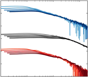
The higher wavenumber spectral characteristics and the collapse with  $kz$ is also further elucidated by plotting the inner-scaled compensated spectra in a log–linear form as shown in figure 10 which encompasses the region near the bed. The compensated velocity spectra appear to begin to flatten at high wavenumbers, thus consistent with the Kolmogorov model
 $k^{-5/3}$ prediction. The inner-scaled shear stress spectra decay more rapidly and when multiplied by
 $(kz)^{-7/3}$ align well with the predictions of Wyngaard & Coté (Reference Wyngaard and Coté1972) at similarly high wavenumbers. This result is consistent with tidal channel measurements by Bowden & Ferguson (Reference Bowden and Ferguson1980) and Lien & Sanford (Reference Lien and Sanford2000), as well as high Reynolds number data wind tunnel data by Saddoughi & Veeravalli (Reference Saddoughi and Veeravalli1994), for which isotropy was first observed for
 $kz$ between 5 and 7.5. Additionally, the tendency of the streamwise spectra to begin to flatten at lower values of
 $kz$ than the wall-normal spectra, is also consistent with the literature. The observations here, therefore, provide further support for the universality of the higher wavenumber spectral characteristics of wall turbulence.
Premultiplied inner-scaled wavenumber spectra. Spectra correspond to  $z/\delta =0.16$ to 0.34, with intervals of
 $z/\delta =0.06$ and are plotted progressively darker as
 $z$ is increased.

4.4. Scaling near the free surface
Finally, the turbulence scaling near the free surface is considered. Figure 11 shows the wavenumber spectra  $\phi (k)$ at various distances from the mean free surface (
 $z'=\delta -z$). Plotted in this way, the velocity spectra and Reynolds stress spectra collapse at high wavenumbers, implying that
 $z$ scaling is no longer relevant at these large distances from the seabed. It is also evident that the wall-normal spectra and, therefore, the wall-normal intensities, are strongly attenuated at low wavenumbers for distances of approximately
 $z'/\delta <0.3$. Here, we hypothesise that
 $z'$ is an appropriate length scale for the wall-normal spectra at low wavenumbers, as it is shown to collapse the spectra in that region (dashed lines). In comparison, the streamwise and Reynolds shear stress are comparatively less affected by the surface. It suggests that near the free surface the large scale eddies are elongated with a pancake-like form. The spectral characteristics are, therefore, qualitatively consistent with that expected based on the shear-free boundary model of Hunt & Graham (Reference Hunt and Graham1978). It can also be noted, that the wall-normal spectra closest to the free surface (which are not affected by spatial non-homogeneity) also show a peak at higher wavenumbers of around
 $k=0.3$. This is indicative of energy from surface waves with periods of approximately
 $8\ \textrm {s}$ which have only limited effect on the turbulence structure through the water column. By integrating the spectra the contribution from surface waves to the intensities was confirmed to be relatively small (i.e. less than 5 % for the smallest
 $z'$ considered), as the intensity is dominated by energy at low wavenumbers.
Streamwise, wall-normal and Reynolds shear stress spectra towards the free surface. Spectra correspond to  $z'/\delta =0.12$ to 0.36, with intervals of
 $z'/\delta =0.06$ and are plotted progressively darker as
 $z'$ is increased.

As an initial attempt at evaluating the theory by Hunt & Graham (Reference Hunt and Graham1978) for predicting the wall-normal turbulence quantities, figure 12 shows the measured and estimated intensities and integral length scales (defined as  $L_{w}=({{\rm \pi} \phi _{ww}(k\rightarrow 0)})/{2\overline {w^2}}$). The quantities are presented as ratios of the free-stream (unblocked) values,
 $\overline {w^2}_\infty$ and
 $L_{u\infty }$. For a relatively shallow tidal channel these free-stream values are difficult to obtain due to the contribution from bottom shear becoming more significant with increased distance from the free surface. Here, we have obtained
 $\overline {w^2}_\infty =0.03\ \textrm {m}^2\,\textrm {s}^{-2}$ using a best fit to the intensity ratios which is considered to be realistic. The streamwise integral scale
 $L_{u\infty }$ has been taken as equal to the channel depth
 $\delta$. The theoretical predictions are based on a free-stream turbulent field that is homogenous and isotropic, described by the von Kármán spectral model. On this basis, the agreement demonstrated between the experimental and theoretical results is encouraging.
Measured and theoretical variation of the wall-normal integral length scale  $L_{w}/L_{u,\infty }$ (blue) and intensity ratios
 $\overline {w^2}/\overline {w^2}_\infty$ with distance from the free surface. Experimental data are denoted by ‘o’ and ‘+’ symbols. Theoretical predictions based on the shear-free boundary model of Hunt & Graham (Reference Hunt and Graham1978) are shown by solid lines (length scales) and dashed lines (intensities).

5. Conclusion
This experiment has provided unique measurements of turbulence in a near canonical channel flow, where the boundary layer occupied the entire water column and at Reynolds numbers an order of magnitude larger than typically attained in the atmospheric boundary layer. The profiles of the mean velocity, turbulence quantities and spectra lend experimental support for the applicability of the wall-similarity, attached-eddy and spectral scaling hypotheses at very high Reynolds numbers and the universality between geophysical flows. Attenuation of the wall-normal velocity spectra near the free surface is, however, a differentiator between tidal channels and the atmospheric boundary layer. Support is demonstrated for the use of theoretical models based on a plane slip surface in predicting the variation of intensities and length scales near the free surface.
Acknowledgements
The provision of the data by SIMEC Atlantis Energy is gratefully acknowledged. The authors also thank I. Marusic, C. Bluteau, A. Zulberti and the anonymous reviewers of the manuscript for their comments.
Declaration of interests
The authors report no conflict of interest.



