INTRODUCTION
One of the primary goals in marine ecology is the determination of factors responsible for the generation of observed spatial patterns (Sokal & Wartenberg, Reference Sokal, Wartenberg, Griffith and Mackinnon1981). For marine macrobenthic invertebrates, such patterns are ultimately the result of a complex interaction of a number of processes operating both within the water column and the sedimentary environment. At large spatial scales for example, gradients such as temperature, salinity and depth generally produce changes in species distributions, assemblage structure and functioning, while changes in sediment characteristics are thought to greatly influence assemblage structure at more local scales (Holme, Reference Holme1961; Platt & Sathyendranath, Reference Platt, Sathyendranath, Giller, Hildrew and Raffaelli1992; Gray, Reference Gray2001; Giberto et al., Reference Giberto, Bremec, Acha and Mianzan2004; Bremner et al., Reference Bremner, Rogers and Frid2006; Labrune et al., Reference Labrune, Gremare, Amoroux, Sarda, Gil and Taboada2007). However, a number of studies have reported a poor correlation between invertebrates and sediment characteristics at such scales, indicating that the precise relationship between benthic community composition and specific sediment properties is poorly understood (Buchanan, Reference Buchanon1963; Day et al., Reference Day, Field and Montgomery1971; Newell et al., Reference Newell, Seiderer and Hitchcock1998). Attempts to resolve this must also take into account the influence on seabed substrate of hydrodynamic properties, especially wave and tidal current action. Consequently, most studies have concluded that explanations for the complexity of soft-bottom communities defy any simple paradigm relating to a single factor and that, in addition to sediment granulometric properties, complex shear forces at the sediment–water interface are likely to be important in controlling food availability, larval settlement, pore-water flow and microbial food availability (Snelgrove & Butman Reference Snelgrove and Butman1994; Newell et al., Reference Newell, Seiderer and Hitchcock1998).
In the European seas, the English Channel represents a transitional zone between the temperate and boreal regions (Sanvicente-Anorve et al., Reference Sanvicente-Anorve, Lepretre and Davoult2002) and, owing to considerable hydrographic variations along its length, provides an interesting environment for the study of macrofaunal distribution trends and controlling factors (Holme, Reference Holme1961). The western part of the Channel, particularly the area south of Plymouth (location of the Marine Biological Association of the United Kingdom) has been studied over many years, the earliest dating as far back as Allen (Reference Allen1899). The macrobenthic fauna of the mid- and eastern English Channel, however, was not formally studied until many years later. Holme (Reference Holme1966) concentrating solely on the larger molluscs and echinoderms, analysing 311 samples on a grid covering the whole Channel. In the eastern Channel, recent studies aimed at mapping macrofaunal species and assemblage distributions, have tended to focus on specific areas such as, for example, Hastings to the French–Belgian border (Sanvicente-Anorve et al., Reference Sanvicente-Anorve, Lepretre and Davoult2002), or the central part of the eastern Channel (James et al., Reference James, Coggan, Blyth-Skyrme, Morando, Birchenough, Bee, Limpenny, Verling, Vanstaen, Pearce, Johnston, Rocks, Philpott and Rees2007). Other studies have been undertaken primarily to assess the impacts associated with human activities such as aggregate extraction (Desprez, Reference Desprez2000; Boyd et al., Reference Boyd, Limpenny, Rees, Cooper and Campbell2003; Cooper et al., in press) and, more inshore, dredged material disposal (Anonymous, 2005) and scallop fishing (Kaiser et al., Reference Kaiser, Armstrong, Dare and Flatt1998).
The aim of the present study was to identify the macrofaunal assemblages and species distributions along the whole of the Channel north of the median line, from the Dover Strait to south of Penzance, and, using uni- and multivariate analyses, to investigate which environmental factors affect assemblages at this scale.
MATERIALS AND METHODS
Study area and sampling design
The environmental characteristics of the English Channel have previously been documented in detail by Holme (Reference Holme1961, Reference Holme1966) and Pingree (Reference Pingree, Banner, Collins and Massie1980). Generally, these studies indicate that there is a large east–west change in physical conditions. The western half of the English Channel is relatively deep (80–100 m) with relatively slow tidal streams (0.5–0.8 m s−1); these increase in the mid-Channel (1.5–2.5 m s−1) where water depths average 60 m. The eastern English Channel is characteristically 40–50 m deep with tidal streams around 0.8 m s−1. In summer, there is a distinct thermocline in the western English Channel, bottom temperatures being several degrees below those of the surface. As water passes west to east along the English Channel, this stratification is broken down so that there is complete mixing of the water in the mid- and eastern English Channel. Summer surface water temperatures in the eastern English Channel may be a little warmer than those in the west but much lower in winter. Thus, the annual range in bottom temperatures in the western English Channel is much less than that in the east (Holme, Reference Holme1966).
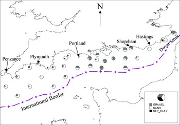
The present study comprises 31 stations along the English section of the English Channel, from the most westerly south of Penzance to the most easterly at the Dover Strait (Figure 1). This area, therefore, covers the whole length of the English Channel according to the arbitrary boundaries defined by Pingree (Reference Pingree, Banner, Collins and Massie1980). International Council for the Exploration of the Sea (ICES) rectangles were used as a basis for sampling, stations being located at intervals of 0.25° latitude and 0.5° longitude at the centre of each rectangle. Due to the irregularities of the coastline, some stations are more opportunistically located (e.g. in the region of the Isle of Wight) to ensure an approximately even spatial coverage.
Spatial distribution of major sediment types throughout the survey area.

Sampling and sample processing
Samples for the macrofauna and sediments were taken during June and July 2005 using a 0.1 m2 Hamon grab deployed from RV ‘Cefas Endeavour’. This device was chosen following its previous success in sampling the sand/gravel sediments of the English Channel (Oele, Reference Oele1978; Boyd et al., Reference Boyd, Barry and Nicholson2006; Cooper et al., in press). Stations were located using a differential Global Positioning System and the ship's TOWER© software that logs the position of each sample. The vessel is maintained in position during grab deployments using dynamic positioning. Stations were set as waypoints with the grabs being taken within a 50 m bullring. The total volume of each of the 3 replicate grab samples was estimated to ensure it exceeded 5 l (Boyd et al., Reference Boyd, Limpenny, Rees, Cooper and Campbell2003) and a 500 ml sub-sample of sediment removed for particle size analysis. The remaining sample was then washed over 5 mm and 1 mm mesh sieves to aid the sorting process. The retained macrofauna were fixed in a 4% formaldehyde solution for later identification (to the lowest taxonomic level (predominantly species)) and enumeration in the laboratory. Colonial species were recorded as present.
The sediment sub-samples removed for analysis of particle size distribution were initially wet sieved on a 500 µm stainless steel test sieve using a sieve shaker. The <500 µm fraction was then freeze-dried, weighed and a sub-sample analysed using a Coulter LS 130 Laser-Sizer. The >500 µm fraction was oven dried at 80°C for 12 h and then sieved over a range of test sieves down to 500 µm at 0.5 phi intervals. The sediment retained on each sieve was weighed to the nearest 0.01 g and the results recorded. The results from these analyses were combined to give a full particle size distribution. The mean particle size and sorting values were also calculated. For the present paper, data from the three replicates were averaged for each station.
At each station, a 0.5 km transect was surveyed using multibeam sonar collecting co-located bathymetry and backscatter information, allowing the seabed morphology and complexity in the vicinity of the grab stations to be characterized over larger spatial areas. The bathymetry allows the construction of a 3D surface to visualize the seabed topography, while backscatter strength is a proxy for sediment type, with harder grounds returning a stronger backscatter. The data were collected using a Kongsberg Simrad EM3000D™ multibeam echosounder with data processing performed using CARIS HIPS/SIPS and visualised using IVS 3D Fledermaus.
Data analysis
Normalized principal components analysis (PCA) was used to investigate the variations in environmental conditions over the survey area and to determine which variables differed the most between stations (Pielou, Reference Pielou1984). The environmental factors included depth, a number of derived granulometric parameters (e.g. % silt, % gravel, sorting coefficient, skewness and kurtosis), together with modelled parameters such as tidal stress, wave stress and a stratification index. Tidal parameters were generated using a 3D hydrodynamic model (Davies & Aldridge, Reference Davies and Aldridge1993), run in depth-integrated form on an approximately 3.5 km resolution grid covering the European continental shelf. A formal validation procedure was not carried out. However, distributions of tidal amplitude and phase were plotted and were found to be in close visual agreement with known distributions of these quantities (e.g. Pingree & Griffiths, Reference Pingree and Griffiths1978). Tidal bed stress was derived from the M2 tidal constituent (the largest component on the European continental shelf). The amplitude of the depth mean M2 tidal ellipse at the grid point nearest to the survey station was calculated. The peak M2 velocity (that aligned along the major axis of the tidal ellipse) was converted to a bed shear stress using a standard quadratic formulation with drag coefficient CD = 0.0025.
The stratification parameter ‘S’ was derived from the formulation presented in Pingree & Griffiths (Reference Pingree and Griffiths1979), using modelled M2 tidal velocities and measured depths at the benthic stations.
Average and peak wave stress were calculated from a one-year model run covering the period September 1999 to September 2000, on an approximately 12 km grid, using the WAM spectral wave model run at the Proudman Oceanographic Laboratory (Osuna & Wolf, Reference Osuna and Wolf2004). Instantaneous wave stress was calculated from the significant orbital velocity at the bed using a standard quadratic formulation with friction factor (fw) as given for rough beds by Swart (Reference Swart1974). A constant bed grain size roughness corresponding to 0.1 mm sand was assumed. Average and peak values of the wave stress were calculated at the grid point nearest to the benthic station to obtain the values used in this study.
The relationship between biological communities and temperature is complex and there are a large number of possible permutations (maximum or minimum winter or summer temperature, temperature range, etc.) which may potentially affect the biota. Such parameters generally vary along the English Channel and, consequently, the longitudinal position of each station was included into the environmental matrix as a surrogate for temperature-related properties. The inclusion of a stratification parameter further encapsulated the variability of temperature-related factors along the English Channel for this study.
The macrofaunal data were primarily analysed using a multivariate community approach using the software packages Minitab™ v13.0 and PRIMER© v6 (Clarke & Warwick, Reference Clarke and Warwick1997). A Bray–Curtis similarity matrix was produced based on the square root-transformed abundance data (the replicate data were averaged within stations). Cluster analysis (group average; Lance & Williams, Reference Lance and Williams1967) was conducted using the similarity matrix to produce a dendrogram and non-metric multidimensional scaling (MDS) was performed to produce an ordination plot. Following clustering, a series of ‘similarity profile’ (SIMPROF) permutation tests were conducted to look for statistically significant evidence of genuine clusters in the community data. The similarity percentages program SIMPER was then used to identify the level of within-group sample similarity and the species responsible for defining group identity. This allowed the description of the main biological assemblages for the English Channel.
Relationships between the biological and environmental data were investigated using both univariate and multivariate approaches. Backward stepwise regression analysis was conducted to determine significant relationships between physical variables and univariate indices of community structure (total density, number of species, Shannon–Wiener diversity and biomass). Multivariate approaches included firstly the RELATE test to determine the significance of any relationships between the similarity matrices underlying the macrofaunal and environmental data. Secondly, in order to gain a further insight, the BIOENV procedure was used to identify which of the tested environmental variables best explained the observed patterns in macrofaunal community distribution. This was achieved by selecting subsets of the available variables that maximized the rank correlations between the two matrices. Longitudinal position of each station was included in the set of explanatory variables for the BIOENV procedure to determine the extent to which geographical position influenced community structure. The mean values of each influential environmental variable were then expressed for each macrofaunal assemblage and statistical differences investigated using a Kruskal–Wallis test.
RESULTS
Sediments and physical conditions
The seabed sediments of the study area varied from fine sand to coarse gravels (Figure 1). Sand was generally the dominant component of the sediments at all stations, with gravel noticeably increasing in the middle of the English Channel and the Dover Strait (maximum = 91.6%; mid-Channel) and silt/clay increasing in a small number of more inshore stations (maximum 24.0%; off Rye Harbour, east of Hastings).
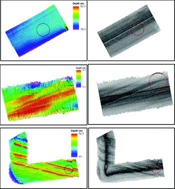
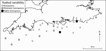
The multi-beam data allow an assessment as to how representative the particle size data for each station is over larger spatial scales. Stations are described as homogeneous, moderately heterogeneous or highly heterogeneous based on the observed degree of spatial variation in sediments seen on the multi-beam bathymetry and back-scatter (Figures 2 and 3). For 18 of the 31 stations, the sediment characteristics described by the grab samples appear to reflect well those over larger areas (i.e. at least a 0.5 km line), for nine stations, some variability is apparent, while for two stations (i.e. inshore of Shoreham and offshore south of the Isle of Wight, Figure 3), the acoustic images indicate that the point at which the grab samples were taken is not representative of (or are fundamentally dissimilar to) the sediment at the wider locale.
Sections of multibeam (left) and backscatter (right) images for 3 stations showing homogeneous (top), fairly heterogeneous (middle) and very heterogeneous (bottom) sediments along a 500 m transect through the sampling stations. (Top: flat seabed of medium sands, middle: topographic relief of 2 m due to layered, outcropping bedrock with a WSW–ENE orientation, widespread presence of coarse gravel, bottom: bedrock outcrops at seabed surface in a WNW–ESE direction. Backscatter in between rocky outcrops indicates coarse sediments.)

Seabed variability in sediments over a 0.5 km line across each station, based on multibeam backscatter.

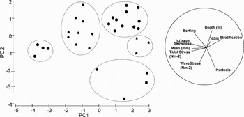
Principal components analysis of the sediment granulometric data and non sediment-related characteristics of each station (e.g. depth, wave and tidal stress, stratification) revealed that the stations could be classed visually into 5 physically-distinct groups (Figure 4). While separation along principal components axis 1 was primarily due to stratification, gravel content and tidal stress, separation along axis 2 mainly reflects variation in depth, sorting, wave stress and kurtosis. As only 58.1% of the total variation is explained by these two axes, the 2-dimensional PCA ordination clearly does not provide a complete explanation of the relationship between the stations (Clarke & Warwick, Reference Clarke and Warwick1997).
Principal components analysis plot based on normalized physical data for all 31 stations. Variables responsible for separating stations are given as vectors whereby the strength of their effect is denoted by the lengths of the lines. Groups have been delineated ‘by eye’ to define physically-comparable stations.

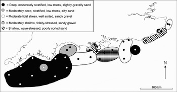
The large inter-sample distances determine that only tentative interpolations can be made in terms of mapping these physical properties (Figure 5). Generally, the western English Channel is characteristically deeper, experiences little wave stress at the bed and there is a high tendency for the waters to stratify. These areas typically have sandy sediments with small yet varying proportions of silt and gravel. The mid- and eastern Channel is somewhat more spatially variable but generally shallower, more tidally- or wave-stressed, with sand or sandy gravel sediments.
Spatial distribution of the 5 physical environments along the survey area. Groups were defined by principal components analysis based on Euclidean distances.

Macrofaunal assemblages
A total of 693 taxa were recorded from the 31 stations sampled. Of these, 546 were non-colonials and 147 were colonials (and therefore necessarily excluded from multivariate analyses of the quantitative data). Examination of the major taxon groups reveals that annelids were the most diverse group with 238 taxa (34.5% of total species), two of which were oligochaetes. Crustaceans accounted for 142 species (20.0% of total), 111 species were molluscs (16.0% of total) and 18 species (2.5% of total) were echinoderms. Taxa which did not fall into any of these main groups accounted for 184 species (27.0% of total), predominantly represented by bryozoans (89 species) and cnidarians (41 species).
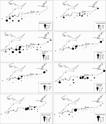
The densities of the eight most abundant species sampled are mapped in Figure 6. These maps indicate that these species do not show random distribution patterns: each is generally clustered at particular stations or regions of the English Channel. Except Balanus crenatus which is generally confined to the mid-Channel sediments, it is notable that these are widely distributed along the English Channel, i.e. none of these species could be regarded exclusively as western- or eastern-Channel species. While Lumbrineris gracilis was found at most stations, Abra alba was sampled only at the more inshore stations.
Density maps of the eight most abundant taxa recorded from the 31 stations. Numbers in legend refer to mean number per grab (0.1 m−2), groups selected to give more-or-less equal counts within groups.

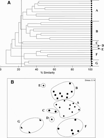
Multivariate data analysis reveals that the similarity between stations is generally low (minimum 6.1%). Such low similarity might be expected given the known magnitude of east–west environmental differences along the English Channel. The dendrogram produced by hierarchical agglomerative clustering using group-average linking produced 7 distinct biological assemblages (at 23% similarity; Figure 7). The SIMPROF test confirmed that these assemblages were significantly different (at 0.1% significance).
(A, B). Dendrogram and MDS ordination plots of biological assemblages in the English Channel. The dendrogram summarizes the results from hierarchical agglomerative clustering using group-average linkage, employing a Bray–Curtis similarity matrix based on root-transformed abundance data. The assemblages A–G are defined as statistically distinct faunal groups by a SIMPROF permutation test at 0.1%, i.e. stations within groups do not statistically differ from each other in multivariate structure at this level of testing.

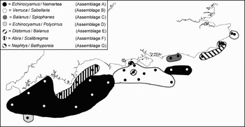
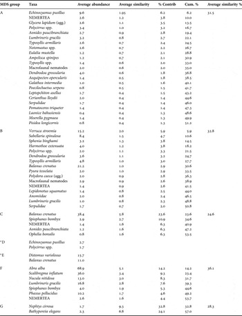
SIMPER tests were conducted to reveal the taxa most responsible for discriminating each macrofaunal assemblage (Table 1). As this was not possible for assemblages D and E (only one station), the most abundant taxa are given. These 7 assemblage types (named according to the two main taxa responsible for discriminating each assemblage; Table 1) are mapped in Figure 8. In summary, the western English Channel is dominated by an Echinocyamus/Nemertea assemblage and the mid-Channel by a Verruca/Sabellaria assemblage. An Abra/Scalibregma assemblage is largely associated with the more inshore waters of the western English Channel. The assemblages of the eastern English Channel become more spatially variable but mainly comprise Nepthys/Bathyporeia and Verruca/Sabellaria assemblages.
Map of the 7 macrofaunal assemblages identified using multivariate analysis. Regions indicating the spatial extent of each assemblage and/or boundaries between neighbouring assemblages have not been determined by interpolation techniques, but by ‘best fit’, and therefore should not be taken as definitive.

Results from SIMPER analysis of macrofaunal data (colonials excluded, data square root-transformed), listing the main characterizing taxa within each assemblage type (to a total of 50% contribution).

* Due to insufficient stations in group, abundances of the two most dominant species are given. Where a species actually comprises a number of microspecies, the term ‘aggregation’ (agg.) is used.
Assemblage characteristics
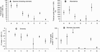
The number of species, abundance, diversity and biomass significantly varied between each of these faunal assemblages (P < 0.001 for each univariate index; Kruskal–Wallis test), see Figures 9 (A–D)). In general, the two most spatially dominant assemblages, the Echinocyamus/Nemertea (group A) and the Verruca/Sabellaria (group B) assemblages were characteristically species-rich (75–80 species 0.1 m−2), exhibited high total abundances and were also the most diverse groups. The Balanus/Spiophanes assemblage (group C) displayed moderate species numbers (35 species 0.1 m−2) and abundances yet possessed the highest biomass (37.8 g wet weight, 0.1 m−2). The Abra/Scalibregma assemblage (group F) exhibited average number of species and diversity with relatively high densities and biomass. The remaining assemblages D, E and G (Echinocyamus/Polycirrus, Distomus/Balanus and Nephtys/Bathyporeia) were comparatively poor faunistically.
(A–D). Univariate indices for each macrofaunal assemblage.

Macrofaunal relationships with environmental variables
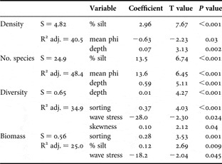
A backward stepwise regression analysis was conducted to explore the significance of any relationships between the four univariate indices of community structure and environmental variables (Table 2). The results indicate that density and number of species were related to mean phi, depth and silt/clay while sorting and wave stress became important variables affecting diversity and biomass. It should be noted that as silt/clay was generally a covariate of sand and gravel (which were therefore excluded from the regression analysis) these can be regarded as also being related to univariate indices of community structure.
Physical variables significantly related to univariate indices of macrofaunal community structure (backward stepwise regression, α = 0.05). This regression removes variables from the regression model for the purpose of identifying a useful subset of predictors. The models below represent those with the highest adjusted R2 values for each univariate index.

S, root mean square error.
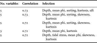
Table 3 displays the best combinations of environmental variables matching the changes in the multivariate biological data. In general, a large amount of the biological variation (correlation coefficient = 0.72) can be explained by 3 variables; additional variables add little to the correlation. These relationships are statistically significant: the 5 models displayed in Table 3 each gave α <0.001 using the RELATE procedure. We conclude, therefore, that the best combination of environmental variables explaining the variability of the multivariate macrofaunal data is depth, mean phi and kurtosis, the former two being significantly correlated with univariate indices.
Combinations of environmental variables yielding best matches of biotic and abiotic similarity matrices, as measured by weighted Spearman rank correlation ρw (BIOENV test).
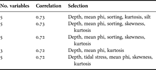
Figure 10 displays an MDS plot based on the best combination of environmental variables (i.e. depth, mean phi and kurtosis) with the station number replaced by its macrofaunal assemblage group. There is a very good agreement between the plot based on these variables and macrofaunal assemblage type. Thus, the overall structure of the species abundance matrix is replicated very well through knowledge of this sub-set of three environmental variables. This conclusion reflects the apparent similarity between the geographical distributions of the various physical environments (Figure 5) and macrofaunal assemblages (Figure 8). Again, sand and gravel were removed from the analysis (covariates with mean phi; ρw = 0.93 and –0.95, respectively), and therefore, are also important variables. It is noteworthy that longitudinal position was not considered to be influential in explaining community patterns along the English Channel.
Multidimensional scaling of stations based on environmental variables that most fully explain the faunal variability; letters refer to the biological assemblage found at each station (variables are depth, mean phi and kurtosis, Spearman rank correlation of 0.72).

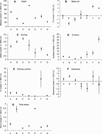
Figure 11 (A–G) presents the mean values of the environmental variables for each macrofaunal assemblage group revealing their differences between assemblage type (α < 0.001 for all variables; Kruskal–Wallis test). The strong relationship between depth and community structure is particularly apparent, with each assemblage type having a narrow depth range, e.g. assemblage D (Echinocyamus/Polycirrus) being restricted to deep waters (approximately 100 m) and assemblages C (Balanus/Spiophanes) and G (Nepthys/Bathyporeia) being restricted to shallow waters (15 and 20 m depth, respectively). Also notable is the increased silt/clay content confined to assemblage F (Abra/Scalibregma) and the high tidal stress (approximately 2.5 Nm−2) experienced at the seabed of assemblages B (Verruca/Sabellaria) and E (Distomus/Balanus) relative to that experienced at the other assemblages, where tidal stress is typically less than 1 Nm−2.
(A–G). Mean physical characteristics for macrofaunal assemblages A–G.

DISCUSSION
Assemblage distributions
This study identified seven distinct macrofaunal assemblages along the English side of the Channel, from south of Penzance to the Dover Strait. These assemblages vary greatly in their spatial extent and geographical distribution. In the south-west, the Echinocyamus/Nemertea assemblage extended from south of Penzance to south of Portland, and offshore south of Shoreham. Inshore along the Devon and Dorset coast, this assemblage gave way to an Abra/Scalibregma assemblage. This community was also found inshore off Rye Harbour, in the eastern English Channel. The second most spatially-extensive community was a Verruca/Sabellaria assemblage dominating the middle of the English Channel, from south of Swanage to south of Shoreham, but also sampled at the eastern limits of the present study in the Dover Strait. The other communities were more isolated, such as an Echinocyamus/Polycirrus assemblage offshore of the Lizard, the Balanus/Spiophanes assemblage inshore of Shoreham, a Nephtys/Bathyporeia assemblage off the Sussex coast, and a Distomus/Balanus assemblage within the Verruca/Sabellaria assemblage south of Poole. Scaling and methodological differences make comparisons of the assemblage structures found here with those of other studies difficult. Sanvicente-Anorve et al. (Reference Sanvicente-Anorve, Lepretre and Davoult2002) used a Rallier du Baty dredge to sample the benthic assemblages of the English Channel east of Hastings and observed a large degree of spatial variability in this part of the Channel. In agreement with the present study, they observed an Abra assemblage inshore along the eastern coast and an assemblage dominated by Nepthys and Bathyporeia offshore. The Verruca/Sabellaria assemblage observed in this study was beyond the eastern limit of their survey area. Brown et al. (Reference Brown, Cooper, Meadows, Limpenny and Rees2002), using a Hamon grab, found that Echinocyamus dominated the sediments offshore of Shoreham (corresponding to the Echinocyamus/Nemertea assemblage) becoming less abundant inshore. Furthermore, Rees et al. (Reference Rees, Pendle, Waldock, Limpenny and Boyd1999) who sampled five stations along the English Channel with a Day grab also found communities dominated by Echinocyamus offshore from Devon and Hampshire, Abra-dominated communities in inshore waters of Devon and Cornwall, and a community comprising high numbers of Nepthys and Bathyporeia to the east of Dungeness. The similarity of the communities found during the present study with those previously reported suggests that such assemblages are spatially (at a local scale) and temporally representative.
A large number of physical factors operate over various spatial scales to influence biological distributions. While temperature differences (east–west in the English Channel) might be expected to induce gradations in the densities of species and/or assemblages, patchiness in sediment types might be expected to induce sharper discontinuities (Holme, Reference Holme1966). These former, large-scale factors have been shown to influence assemblages in the North Sea (Kunitzer et al., Reference Kunitzer, Basford, Craeymeersch, Dewarumez, Dorjes, Duineveld, Eleftheriou, Heip, Herman, Kingston, Niermann, Rachor, Rumohr and de Wilde1992; Callaway et al., Reference Callaway, Alsvag, de Boois, Cotter, Ford, Hinz, Jennings, Kroncke, Lancaster, Piet, Prince and Ehrich2002; Rees et al., Reference Rees, Eggleton, Rachor and Vanden Berghe2007). Holme (Reference Holme1966) described seven patterns of distribution for the whole English Channel based on molluscs and echinoderms. One related to species which were found along the entire length of the English Channel: in agreement with Holme (Reference Holme1966), we found Abra alba and Phaxus pellucidus to exhibit this distribution. The other six patterns discerned by Holme (Reference Holme1966) related to species presences exclusively in one part of the English Channel. For example, Venus striatula represented a western Channel species (being absent from the east), while Spisula elliptica was described as an eastern Channel species. Holme's work, therefore, implied that the majority of the species sampled during his survey of the English Channel showed discrete patterns in which the environmental conditions precluded their occurrence from one or several parts of the Channel. However, such distributions were generally not observed during the present study and the most abundant taxa (except Balanus crenatus which was restricted to the mid-Channel region) were sampled along the entire length, albeit in varying densities (Figure 6). Although a broad difference may be apparent, multivariate analyses revealed that this conclusion regarding species distributions to some extent relates to assemblage structure. For example, the Echinocyamus/Nemertea assemblage, although representing the majority of the western Channel was also observed south of Shoreham, and the Verruca/Sabellaria assemblage which had its western limits south of Poole was also found to be present off the Dover Strait.
The east–west separation in the English Channel characterizing Holme's study employing an anchor dredge, therefore, does not appear so marked for the assemblages sampled by a grab. It is possible, therefore, that different conclusions regarding an east–west difference in the English Channel reflect the differences in sampling gear. For example, while polychaetes formed the largest component of the total taxa in the present study, these were not included in the study by Holme (Reference Holme1966) where larger molluscs and echinoderms were the focus. It is possible that, in contrast to larger species, such smaller infauna show weak relationships with larger-scale, biogeographical factors (e.g. temperature) and sediment characteristics are more important structuring factors. This is supported by Rees et al. (Reference Rees, Pendle, Waldock, Limpenny and Boyd1999) who found, based on sampling using a Day grab, comparable infaunal communities were present around the entire England and Wales coast given comparable sediment types, while the epifaunal assemblages were structured by larger-scale factors and different communities were therefore observed across geographical areas.
A possible alternative explanation for the apparent differences in the regional distributions of species between the present study with earlier studies by Holme (Reference Holme1961, Reference Holme1966) could be related to long term changes in diversity associated with species invasions and extinctions. Current biogeographical research indicates that increased species invasions and extinctions, in relation to increased human impacts, are leading to increased taxonomic similarity of biotas among sites over time. This phenomenon, known as biotic homogenization (Olden & Rooney, Reference Olden and Rooney2006), describing the gradual replacement of regionally distinct communities by cosmopolitan communities, is currently regarded as being widespread in both aquatic and terrestrial systems. While it is not possible to support or refute this as being a possible mechanism for the more widespread distributions of species along the Channel in the present study, this study provides a valuable baseline from which this mechanism can be tested by subsequent temporal sampling (Olden & Rooney, Reference Olden and Rooney2006).
The present study indicated that the English Channel could be classed into five, physically-distinct geographical areas based on sedimentary characteristics (e.g. mean particle size and kurtosis) and non-sediment derived parameters such as depth and bed stress. While deep, moderately stratified, low stress, slightly gravelly sand regions generally typified the western Channel, the physical conditions experienced in the mid- and eastern Channel were more spatially variable. These latter regions were shallower with higher bed stresses and higher gravel contents. The geographical boundaries observed between the physical areas defined here are supported by those observed on the web-based GIS UK SeaMap (Connor et al., Reference Connor, Gilliland, Golding, Robinson, Todd and Verling2006) based on data from a variety of sources using modelling, remote sensing and direct sampling techniques. This agreement adds support to the data obtained during the present study, based largely on sediment grab sampling and Cefas-derived modelled hydrographic data.
Most of the spatial variation in benthic communities was explained by the physical variables, predominantly depth, variables associated with sediment particle size distributions and bed wave and tidal stress. Neither longitudinal position nor the stratification index, both acting as a proxy for temperature variations along the English Channel, explained a significant amount of biological variation. Significant differences in all the physical variables were found between different macrofaunal assemblage types. For example, two assemblages (B and E) were restricted to regions with significantly higher tidal stress conditions relative to other areas, and each assemblage was restricted to a comparatively narrow depth-range (Figure 11). Significant relationships between biota and properties associated with the dynamic nature of the environment were, therefore, found. These relationships also brought about significant differences in macrofaunal assemblage structure. For example, the shallow, wave-stressed and poorly sorted sediments observed at a small number of stations west of the Isle of Wight and off the Sussex coast created a distinct assemblage which typically was faunistically poor in terms of species, abundance and biomass. Thus, the degree of physical disturbance of the sediments expressed in terms of wave and tidal stress provided a convincing explanation of broad trends in the faunal data. This finding is comparable with that of other authors e.g. Warwick & Uncles (Reference Warwick and Uncles1980) who linked variability in the Bristol Channel fauna to bed shear stress arising from tidal action. Cabioch (Reference Cabioch1968) also identified the critical importance of tidal influences on the distribution of benthic species in the English Channel, mediated through their effects on substratum characteristics, particle transport and water mixing. While this holds true for shallow regions, the macrofaunal communities of the English Channel in general were associated predominantly with depth and granulometric properties of the sediments.
Acoustic interpretation: implications for temporal comparisons
Presently, large-scale spatial surveys of biological and physical characteristics ultimately rely on replicated point samples taken close to each other (e.g. several metres in the present study) to represent conditions between nearest stations (between 8 and 27 miles) at this relatively coarse resolution. As a result, any spatial variability between these two scales is clearly unaccounted for. Recent developments in acoustic techniques now allow highly resolved assessments of the physical characteristics of the seabed over large spatial scales and natural biological assemblages have been shown to be relatively consistent within acoustically-similar areas (Brown et al., Reference Brown, Cooper, Meadows, Limpenny and Rees2002; James et al., Reference James, Coggan, Blyth-Skyrme, Morando, Birchenough, Bee, Limpenny, Verling, Vanstaen, Pearce, Johnston, Rocks, Philpott and Rees2007). Within the eastern English Channel, for example, Brown et al. (Reference Brown, Hewer, Meadows, Limpenny, Cooper and Rees2004) and Foster-Smith et al. (Reference Foster-Smith, Brown, Meadows, White and Limpenny2004) characterized the biological habitats within an area of seabed (12 × 4 km) based on the physical maps derived from acoustic data.
The brevity and spatial separation of the acoustic transects sampled in this study preclude any interpolation between stations, but the information acquired does allow us to determine how representative the observed biological communities are over spatial scales somewhat larger than the sampling points, i.e. the area covered by each acoustic transect equates to approximately 150, 000 m2 compared to 0.3 m2 sampled by the grabs. The acoustic data acquired during this study, therefore, explicitly serve a different purpose from the acoustic data used by Brown et al. (Reference Brown, Hewer, Meadows, Limpenny, Cooper and Rees2004) and Foster-Smith et al. (Reference Foster-Smith, Brown, Meadows, White and Limpenny2004) in the eastern English Channel. In the present study, 18 of the 31 stations along the English Channel were described as physically homogeneous over the 0.5 km multibeam transect through the sampling station. Therefore, it may be concluded that the biological assemblages determined at these stations are representative over the 0.5 km line (at least in the direction through which the line was derived). This has practical as well as ecological implications. Subsequent sampling in the general vicinity of these stations is likely to be comparable and, therefore, any changes in communities observed are more likely to reflect real temporal changes (as opposed to artefacts resulting from spatial variability). Conversely, two stations (50.24991N 1.49777W; 50.77322N 0.27270W WGS84) were described as highly heterogeneous and, therefore, the biological communities sampled at these stations are unlikely to reflect those outside the station itself. In such areas, subsequent sampling for temporal comparisons must either ensure that exactly the same locations are sampled as those in the present study or temporal comparisons using such stations are made with great caution.
ACKNOWLEDGEMENTS
This survey represents a component of a larger, on-going study to map the macrofaunal communities of the entire UK coastal and offshore area (i.e. North Sea, English Channel, Celtic, Irish and Malin Seas) and was funded by the Science Directorate of the UK Department for Environment, Food and Rural Affairs (project code ME3112). Earlier versions of this manuscript were greatly improved following comments by Dr Roger Coggan and two anonymous referees. We would like to thank a number of Cefas staff involved in sample collection and processing, and Dr John Aldridge for providing the modelled physical data.