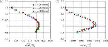
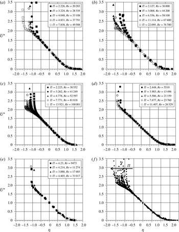
1 Introduction
It is well known that a turbulent boundary layer can undergo flow separation if exposed to an adverse pressure gradient (APG) of sufficient magnitude and/or duration. Turbulent boundary layer separation due to an APG is a common occurrence in many engineering flows and is typically associated with off-design conditions that result in a degradation of device performance. In many cases such as gas turbine blades or helicopter rotors, the pressure gradient varies both spatially and temporally and can lead to an unsteady turbulent boundary layer separation/reattachment cycle. An improved understanding of the underlying flow physics is a prerequisite to the development of effective flow control strategies.
1.1 Generic features of APG turbulent boundary layers
Because of their practical importance, APG turbulent boundary layers have been the focus of many previous studies, and many generic features are now well recognized. The mean velocity profile has been shown to develop a large outer wake region with increasing APG (Samuel & Joubert Reference Samuel and Joubert1974). Deviation from the classic logarithmic law-of-the-wall mean velocity profile has been documented in direct numerical simulations by Spalart & Watmuff (Reference Spalart and Watmuff1993), Nagano, Tsuji & Houra (Reference Nagano, Tsuji and Houra1998) and Lee & Sung (Reference Lee and Sung2009) as well as in experiments by Harun, Monty & Marusic (Reference Harun, Monty and Marusic2010). These studies all show that the APG data exhibit a systematic shift below the classical log-law profile as the strength of the APG increases. This aspect was also clearly documented by Nagib & Chauhan (Reference Nagib and Chauhan2008) in their investigation into the variation of the Karman constant in wall-bounded canonical flows.
The effect of the APG on the turbulent stresses is also quite significant. For example, it has been shown that an APG reduces the turbulent kinetic energy in the near-wall region. In fact, Skåre & Krogstad (Reference Skåre and Krogstad1994) showed that a strong APG gives rise to turbulent diffusion away from the central part of the boundary layer and towards the wall. This was found to be associated with a reduction in both near-wall anisotropy and streamwise correlation length scale. The diffusion originated from a source of turbulence production located near
 $y/\unicode[STIX]{x1D6FF}=0.45$
(where
 $y$
and
 $\unicode[STIX]{x1D6FF}$
are the wall-normal spatial coordinate and boundary layer thickness, respectively). Krogstad & Skåre (Reference Krogstad and Skåre1995) subsequently showed via quadrant-splitting conditional measurements that, unlike the zero pressure gradient (ZPG) boundary layer in which ejection (i.e. quadrant 2) and high-speed sweep (i.e. quadrant 4) motions are of nearly equal importance in the near-wall region, the strong APG boundary layer is entirely dominated by quadrant 4 motions. For the strongest quadrant 4 motions, quadrant 1 events were also found to occur, which the authors interpreted as due to a reflection of coherent structures from the wall. These observations are in stark contrast to results for strong favourable pressure gradient (FPG) turbulent boundary layers obtained by Bourassa & Thomas (Reference Bourassa and Thomas2009), in which quadrant 4 motions were virtually eliminated, while infrequent but strong quadrant 2 motions persisted.
Several previous APG turbulent boundary layer studies have also documented the development of an outer turbulence intensity peak, which develops above the near-wall peak. The outer peak tends to become wider and stronger with the strength of the imposed APG, and moves farther away from the wall with increasing streamwise distance. For example, Dengel & Fernholz (Reference Dengel and Fernholz1990) first showed that as the boundary layer approaches separation and the local maximum of the mean velocity gradient,
 $\unicode[STIX]{x2202}\overline{U}/\unicode[STIX]{x2202}y$
, moves away from the wall, the maximum Reynolds stress and the peak turbulence production also shift away from the wall and move towards the middle of the boundary layer. The development of an outer turbulence peak is also readily apparent from comparison of premultiplied energy spectrum maps of the streamwise velocity component for APG and ZPG boundary layers as presented by Harun et al. (Reference Harun, Monty and Marusic2010, Reference Harun, Monty, Mathis and Marusic2013). In the former reference, it is shown that the effect is fairly insensitive to Reynolds number variation and is thus primarily associated with the APG. Shah, Laval & Stanislas (Reference Shah, Laval and Stanislas2009) examined several previous APG turbulent boundary layer studies and showed that the development of an outer turbulence intensity peak is common to both straight and curved-wall APG turbulent boundary layer flows, and concluded that it is a direct consequence of the imposed APG.
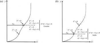
Previous studies have also suggested that an underlying flow instability is responsible for the development of the outer turbulence intensity peak. Song, Degraaff & Eaton (Reference Song, Degraaff and Eaton2000) investigated a turbulent boundary layer that separates, reattaches and recovers over a smoothly contoured ramp followed by a downstream flat plate. It was observed that the peaks of the streamwise-component normal stress and shear stress shift outward away from the wall as the flow develops downstream, and that the peaks remain in alignment with the inflection point in the mean velocity profile, all of which suggest the role of an underlying instability. At the separation location, the peak production of turbulent kinetic energy shifts outward into the separated shear layer over a much wider portion of the boundary layer. There is virtually zero production near the wall at separation. These observations were used to develop an inflection point scaling valid for the region of separated flow. Song & Eaton (Reference Song and Eaton2004) scaled the Reynolds stress profiles from the separated flow region with a velocity scale equivalent to the inflection point mean velocity at reattachment and a length scale given by the wall-normal location of the inflection point. The Reynolds stress profiles collapsed using the inflection point scaling, indicating that large-scale low-frequency motions of the separated shear layer are the dominant contributors to the turbulence production in the separated flow. More recently, George, Stanislas & Laval (Reference George, Stanislas and Laval2012) also highlighted evidence in the literature for the development of an outer turbulence peak associated with the imposition of an APG. It was noted that in all cases where the mean velocity profile becomes inflectional, the location of the inflection point corresponds quite closely to the observed peak in the streamwise turbulence intensity. This suggests the potential role of an underlying instability mechanism in APG turbulent boundary layer development.
1.2 Unsteady turbulent boundary layer separation
Several experimental studies of unsteady attached and separating turbulent boundary layers have been undertaken, and many of the earliest studies were reviewed by Carr (Reference Carr1981). In general, these experiments have sought to examine the response of turbulent wall layers on flat plates, diffusers, pipes and airfoils to unsteady pulsations of the free-stream velocity or to unsteady pressure gradients imposed by various types of oscillatory mechanical elements. One important parameter used in characterizing the unsteady boundary layer is the non-dimensional reduced frequency, defined as
 $$\begin{eqnarray}k\equiv \frac{\unicode[STIX]{x1D714}\ell }{2U_{\infty }},\end{eqnarray}$$
where
 $\unicode[STIX]{x1D714}=2\unicode[STIX]{x03C0}\,f$
is an imposed angular frequency,
 $\ell$
is a relevant length scale (e.g. chord length in the case of a pitching airfoil) and
 $U_{\infty }$
is the free-stream velocity. The reduced frequency represents the ratio of the convective time scale,
 $\ell /U_{\infty }$
, to the imposed unsteady time scale,
 $1/\unicode[STIX]{x03C0}\,f$
. As noted by Leishman (Reference Leishman2000), when the imposed unsteady time scale is less than 20 convective time scales, i.e.
 $k>0.05$
, the flow is generally considered to be unsteady.
In one of the earliest studies, Karlsson (Reference Karlsson1959) exposed a flat-plate ZPG turbulent boundary layer to large-amplitude (up to 34 % of free stream) periodic oscillation of the external flow. The measurements were conducted in an equivalent reduced frequency range of
 $k=0.56$
–82. This study demonstrated that the time-averaged mean velocity profiles were nearly the same as the steady flow case with an equivalent mean free-stream velocity. The effect of the oscillations on the in-phase and out-of-phase boundary layer fluctuations over the range of frequencies was smaller than the experimental error. Parikh, Reynolds & Jayaraman (Reference Parikh, Reynolds and Jayaraman1982) conducted experiments in a water tunnel with imposed oscillations over a reduced frequency range of
 $k=0.65$
–5.2. The time-averaged mean velocity and turbulence intensity profiles were also found to be unaffected by the imposed oscillations. The Reynolds stresses from the organized coherent velocity fluctuations were negligible compared with the Reynolds stresses due to random fluctuations. Measurements on a NACA 0012 airfoil with unsteady flow generated by a rotating elliptic cylinder, conducted by Covert & Lorber (Reference Covert and Lorber1984), also showed that for moderate APGs the mean velocity profiles were independent of the reduced frequency over a range of
 $k=0.5$
–6.4. However, for an APG sufficiently large to produce incipient separation, the time-averaged mean profiles varied from the equivalent steady-state profile as the frequency was increased. For low frequencies, the phase-averaged velocity profiles were highly dependent on the pressure gradient.
Additional studies with APGs large enough to produce flow separation show strong unsteady viscous effects, especially in the near-wall region. These studies show that it is possible to obtain reverse flow in the near-wall region during some portion of the cycle without the occurrence of large-scale separation from the surface. Despard & Miller (Reference Despard and Miller1971) measured instantaneous velocity profiles of an unsteady separating boundary layer with hot-wire arrays to show that the vanishing wall shear and appearance of reversed flow do not necessarily coincide with separation. They proposed a separation criterion based on the observation of shear stress at the wall that was less than zero throughout the entire oscillation cycle. Koromilas & Telionis (Reference Koromilas and Telionis1980) conducted an experimental investigation of unsteady boundary layer flows over convex contours for various APGs. Their results showed that separation responds with time lag to external disturbances, and there is a characteristic inertia in the response of separation. Simultaneous flow visualization and laser Doppler velocimetry (LDV) measurements showed that an upstream propagating separation is preceded by a layer of reversed flow as thin as 5 % of the boundary layer thickness. These experiments underscore the importance of not using zero skin friction as a criterion for separation in unsteady boundary layer flows. The Moore–Root–Sears model uses an alternative criterion to define an unsteady separation point. This model proposes that an unsteady separation point is characterized by zero skin friction and zero velocity at some point in the boundary layer in the reference frame of an observer moving with the separation point (see Sears & Telionis Reference Sears and Telionis1975).
1.3 Objectives and organization
In this paper, the experimental results from an investigation into a turbulent boundary layer developing in a non-equilibrium APG that varies in both space and time are presented. The experimental facility provides flat-plate turbulent boundary layer growth followed by a convex ramp section that allows for the development of a turbulent boundary layer under APG conditions. An airfoil in a post-stall configuration, equipped with leading edge dielectric barrier discharge (DBD) plasma flow control, located above the ramp section is used to impose an unsteady APG on the convex ramp flow. The plasma flow control is used to periodically attach and separate the airfoil suction surface flow, which serves to impose a time-dependent APG on the convex ramp turbulent boundary layer below. The time-dependent pressure gradient gives rise to an unsteady separation/reattachment cycle near the aft portion of the ramp. Full details regarding the experimental facility and model geometry are described in § 2.
The response of the turbulent boundary layer to the imposed unsteady APG at selected streamwise locations on the convex ramp is documented. Upstream locations on the ramp remain attached throughout the unsteady cycle while downstream stations exhibit an unsteady separation/reattachment cycle. Alternately, at fixed times (i.e. phase) during the unsteady cycle, the spatial development of the boundary layer under APGs of different strengths is examined.
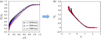
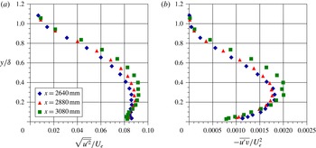
It will be shown from the experimental results that the unsteady APG turbulent boundary layer flow physics becomes dominated by an inviscid instability mechanism associated with an embedded shear layer. This occurs even in the absence of separation. Length and velocity scales based on the embedded shear layer instability are used to develop an embedded shear layer scaling which is shown to provide excellent collapse of both the mean and phase-averaged velocity, turbulence intensity and Reynolds shear stress profiles. The generic applicability of this scaling to APG turbulent boundary layers is demonstrated.
In the following section, the experimental apparatus is described in detail along with the flow diagnostics utilized in the experiments.
2 Experimental facility and conditions
2.1 Wind tunnel and experimental configuration
The experiments were conducted in a subsonic open-return wind tunnel located in the Hessert Laboratory at the University of Notre Dame. The wind tunnel has an inlet contraction ratio of 20 : 1 and contains a series of 12 turbulence management screens resulting in free-stream turbulence levels of less than 0.1 % for frequencies between 10 Hz and 10 kHz. Air is drawn through the inlet by an eight-bladed fan connected to an 18.6 kW AC induction motor. The test section is
 $0.610~\text{m}\times 0.610~\text{m}$
(
 $2~\text{ft}\times 2~\text{ft}$
) in cross-section and 1.83 m (6 ft) in length. One test section sidewall and the ceiling have large plate glass inserts in order to provide optical access to the flow field. The temperature is maintained constant during wind tunnel operation.
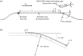
A schematic of the full model configuration is shown in figure 1(a). A fifth-order polynomial shaped contour, constructed from sheet metal, smoothly brings the flow from the floor of the wind tunnel inlet up to the level of a flat boundary layer development plate. At the termination of the contour, the boundary layer is tripped with a 50.8 mm (2 in.) wide strip of distributed sand grain roughness with an average roughness element size of
 $46~\unicode[STIX]{x03BC}\text{m}$
. The boundary layer development plate is 0.914 m (36 in.) long and spans the entire test section of 0.610 m (24 in.).
The boundary layer development plate is followed by a convex ramp of constant radius of curvature,
 $R=0.510$
m (20.08 in.). As shown in figure 1(b), the convex ramp geometry consists of multiple
 $5^{\circ }$
inserts, constructed using an epoxy mould, which smoothly connect together to create a circular arc that can be controlled in
 $5^{\circ }$
increments based on the number of inserts installed. At each ramp insert junction, great care was taken to ensure an aerodynamically smooth transition between the inserts. The results presented in this paper are for a fixed configuration with
 $\unicode[STIX]{x1D703}=25^{\circ }$
(as defined in figure 1
b). Following the curved section of the ramp, a 0.152 m (6 in.) flat section extends the ramp section to the tunnel floor. As shown in figure 1(b),
 $x$
denotes the streamwise spatial coordinate along the convex ramp surface while the total length of the ramp, consisting of circular arc and straight sections, was
 $L=0.375$
m. Measurements were performed over the region
 $0\leqslant x/L\leqslant 1$
. A fairing, constructed from Teflon sheeting with matched derivative end conditions, smoothly transitions the end of the ramp back to the floor of the wind tunnel test section, as shown schematically in figure 1(a). No measurements were performed on this fairing section.
A NACA 0015 airfoil model positioned in a nose-down post-stall configuration and equipped with leading edge DBD plasma flow control was located above the ramp section. Plasma flow control on the airfoil is not a focus of this experimental study but was used simply as a means to impose an unsteady APG on the ramp turbulent boundary layer below (without the use of any moving parts) while maintaining a constant approach flow. Those readers unfamiliar with DBD plasma actuators are referred to comprehensive reviews on the subject provided by Moreau (Reference Moreau2007), Corke, Post & Orlov (Reference Corke, Post and Orlov2009) and Corke, Enloe & Wilkinson (Reference Corke, Enloe and Wilkinson2010).
(a) Schematic of the experimental apparatus. (b) Schematic of the convex ramp geometry and streamwise coordinate.

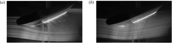
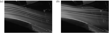
With the plasma off and the airfoil flow fully separated, the APG turbulent boundary layer on the convex ramp remains attached but near a state of incipient detachment. With airfoil leading edge plasma flow control on, the flow attaches to the airfoil suction surface. This has the effect of imposing a rapid increase in magnitude of the APG over the convex ramp section below, thereby precipitating turbulent boundary layer separation near the end of the ramp. Figure 2 compares visualization images of flow over the airfoil in the plasma-off and plasma-on cases. The influence of the leading edge plasma in reattaching the airfoil flow is apparent. Figure 3 presents corresponding images of the external flow over the convex ramp. The plasma-on case, which corresponds to a more severe APG, gives rise to flow separation on the aft section of the ramp. By temporally oscillating the leading edge airfoil plasma flow control, the ramp boundary layer is caused to undergo an unsteady separation and reattachment cycle. Since the region of oscillatory pressure gradient is spatially localized to a specific region of the ramp, the initial flow conditions at the beginning of the ramp are maintained constant in the experiment.
Streakline visualization of the flow over the airfoil for (a) plasma-off (separated flow) and (b) plasma-on (attached flow) cases: chord Reynolds number
 $Re_{C}=1.2\times 10^{5}$
(
 $U_{\infty }=10~\text{m}~\text{s}^{-1}$
).

Streakline visualization of the ramp flow for (a) plasma-off (ramp attached) and (b) plasma-on (ramp separated) cases:
 $U_{\infty }=10~\text{m}~\text{s}^{-1}$
.

The airfoil section was constructed from an epoxy mould with a 0.203 m (8 in.) chord. The airfoil had a span of 0.508 m (20 in.) and terminated in the spanwise direction in thin Plexiglas end plates that served to ensure a two-dimensional airfoil flow. The airfoil was mounted from the test section ceiling, and its mid-chord position (
 $x_{a}$
,
 $y_{a}$
) relative to the beginning of the ramp section was adjustable in both the horizontal (i.e. streamwise) and vertical directions. The airfoil angle of attack relative to the approach flow was also adjustable. For all of the results presented in this paper, the airfoil mid-chord was fixed at
 $x_{a}=216$
mm (8.5 in.) downstream of the convex ramp leading edge and
 $y_{a}=152$
mm (5.98 in.) above it. The airfoil geometric angle of attack with respect to the oncoming flow was fixed at
 $\unicode[STIX]{x1D6FC}=-12^{\circ }$
(nose-down configuration) with maximum blockage of less than 7 %, which posed no detrimental effects to the experimental arrangement.
2.2 Initial conditions for the ramp flow field
Measurements of the ZPG turbulent boundary layer that developed on the plate upstream of the ramp were conducted using constant-temperature hot-wire anemometry. A TSI IFA 100 anemometer and a conventional straight sensor probe (Auspex type AHWU-100) were used for the boundary layer surveys. The probe was traversed normal to the plate using a computer controlled traverse that had a resolution of
 $2.54~\unicode[STIX]{x03BC}\text{m}$
(
 $10^{-4}$
in.) per step.
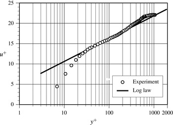
Turbulent boundary layer mean velocity profile upstream of the convex ramp (
 $x/L=-0.085$
).

Approach ZPG turbulent boundary layer characteristics.

The boundary layer characteristics immediately upstream of the ramp section (i.e.
 $x/L=-0.085$
) were found to be identical, regardless of the imposed unsteady pressure gradient on the ramp. These initial boundary layer parameters are summarized in table 1. The parameters presented in this paper correspond to nominal upstream conditions of
 $U_{\infty }=10~\text{m}~\text{s}^{-1}$
and momentum thickness Reynolds number,
 $Re_{\unicode[STIX]{x1D703}}=1600$
just upstream of the convex ramp. The wall-shear stress was based on the Clauser method (and subsequently confirmed via oil film interferometry). Outer variable scaling of the measured mean velocity profile just upstream of the ramp showed very good agreement with the Klebanoff (Reference Klebanoff1955) ZPG profiles obtained at the considerably higher
 $Re_{\unicode[STIX]{x1D703}}=8000$
. Inner variable scaling of the measured mean velocity profile just upstream of the convex ramp is shown in figure 4 and, consistent with the approach Reynolds number, exhibits a limited wall-normal region in good agreement with the classic logarithmic law-of-the-wall profile.
It is important to note that the ratio of initial boundary layer thickness to convex ramp radius
 $\unicode[STIX]{x1D6FF}/R=0.049$
on the circular arc portion, so although there will be an influence of wall curvature on boundary layer development, it will be extremely small compared with the effect of the imposed unsteady APG (see Gibson, Verriopoulos & Vlachos Reference Gibson, Verriopoulos and Vlachos1984; Muck, Hoffman & Bradshaw Reference Muck, Hoffman and Bradshaw1985). As shown in figure 1(b), for
 $x/L>0.6$
the ramp is straight (
 $R\rightarrow \infty$
).
2.3 Airfoil leading edge plasma flow control
The time-dependent pressure gradient imposed on the convex ramp was created by alternately attaching and separating the airfoil flow. As described in § 2.1, this was accomplished by using a DBD plasma actuator positioned at the leading edge of the NACA 0015 airfoil which was cycled on and off at a prescribed frequency.
The dielectric material used for construction of the NACA 0015 airfoil leading edge plasma actuator consisted of two layers of 0.127 mm (0.005 in.) thick Kapton tape between two layers of 0.051 mm (0.002 in.) thick Teflon tape. The Teflon tape protects the Kapton tape from degradation due to the ozone produced by plasma formation (thereby significantly extending the lifetime of the actuator to several days of continuous operation). The leading edge of the airfoil was moulded with a recess of sufficient depth for the actuator to ensure an aerodynamically smooth leading edge surface. The electrodes were made from 0.127 mm (0.005 in.) thick copper foil tape. The covered electrode was 2.54 cm (1 in.) wide and had a span of 35.6 cm (14 in.), while the exposed electrode was 1.27 cm (0.5 in.) wide and had a span of 38.1 cm (15 in.) The electrodes had an overlap of approximately 1 mm (0.039 in) to ensure a uniform DBD plasma discharge throughout the span. Although the spanwise extent of the DBD plasma actuator only covered the central 75 % of the airfoil span, this was sufficient to fully attach the flow over the full extent of the airfoil suction surface.
Previous studies of active leading edge flow control with symmetric and cambered airfoils over a range of chord Reynolds numbers and Mach numbers have shown that the most effective forcing frequency,
 $f$
, occurs when the non-dimensional frequency
 $F^{\ast }\equiv fc/U_{\infty }\approx 1$
, where
 $c$
is the airfoil chord length and
 $U_{\infty }$
is the free-stream velocity (e.g. Seifert et al.
Reference Seifert, Bachar, Koss, Shepshelovich and Wygnanski1993; Seifert, Darabi & Wygnanski Reference Seifert, Darabi and Wygnanski1996; Seifert & Pack Reference Seifert and Pack1999; Patel et al.
Reference Patel, Ng, Vasudevan, Corke, Post, Mclaughlin and Suchomel2008). In this study, when the airfoil plasma actuator was on, it was operated at
 $F^{\ast }=1$
, which, for the conditions of the experiment, corresponded to a physical frequency of
 $f=1/T_{a}=50$
Hz.
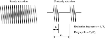
Schematic of quasi-steady and unsteady signals used for plasma actuation.

The DBD plasma a.c. carrier was a negative ramp function of frequency 3.5 kHz and peak-to-peak voltage of 15 kV. The negative ramp function has previously been shown to be optimum in plasma flow control applications (e.g. Thomas et al.
Reference Thomas, Corke, Iqbal, Kozlov and Schatzmam2009). The actuator duty cycle was set at
 $T_{d}/T_{a}=10\,\%$
. Figure 5 contrasts ‘quasi-steady’ and ‘unsteady’ a.c. signals used for plasma actuation and also defines both the plasma excitation frequency and the duty cycle.
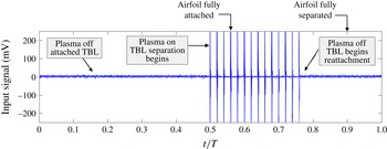
Figure 6 shows one cycle of the periodic signal sent to the airfoil leading edge plasma actuator (prior to amplification). The period of the time series
 $T=1$
s. The mid-point,
 $t/T=0.5$
, represents the stage in the unsteady actuation cycle just prior to plasma initiation, and so the airfoil flow is separated and the APG turbulent boundary layer on the convex ramp is attached. From
 $0.5\leqslant t/T\leqslant 0.75$
, the leading edge plasma actuator is operated in an unsteady mode at
 $F^{\ast }=1$
with an actuation duty cycle of 10 %. As shown in figure 6, the duty cycle for the unsteady separation time scale was fixed at 25 %. Figure 6 indicates the time interval after plasma initiation for the airfoil flow to fully reattach as well as the time interval after extinguishing the plasma for the airfoil flow to separate.
One cycle of the signal sent to the airfoil leading edge plasma actuator (prior to amplification). Here, TBL stands for turbulent boundary layer.

As noted previously, an important and often-used parameter for characterizing unsteady boundary layer behaviour is the non-dimensional reduced frequency,
 $k$
, defined in (1.1). For example, the reduced frequency range relevant to dynamic stall in helicopter rotors is typically quoted in the range
 $k=0.05$
–0.15. In this experiment, the reduced frequency based upon the convex ramp length (
 $\ell =L=37.54~\text{cm}=14.8~\text{in.}$
) was
 $k\approx 0.12$
. This corresponded to a physical cyclic frequency of
 $f_{c}=1$
Hz.
The airfoil reattachment process was documented using flow visualization in conjunction with a Photron FASTCAM SA-1 675K-M1 high-speed camera operated at 2000 fps. High-speed imaging of the airfoil flow indicated that the actuator-induced reattachment process initiated at
 $t/T=0.50$
was complete by
 $t/T=0.56$
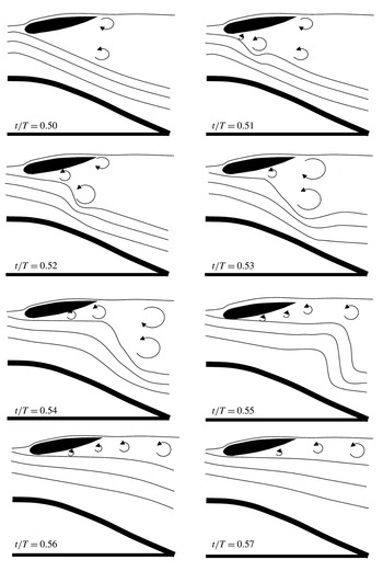
, as is denoted by the arrow in the voltage–time history shown figure 6. This imposes a more severe APG on the convex ramp flow field which leads to boundary layer separation. Figure 7 presents an interpretive sketch of the airfoil flow-field reattachment process based on the high-speed video imaging for the time interval
 $0.5\leqslant t/T\leqslant 0.57$
.
Flow-visualization-based streakline sketches of the airfoil and ramp flow field for the time interval
 $0.5\leqslant t/T\leqslant 0.57$
over which the airfoil flow reattaches.

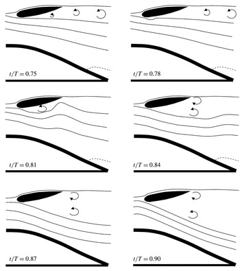
Flow-visualization-based streakline sketches of the airfoil and ramp flow field for the time interval
 $0.75\leqslant t/T\leqslant 0.9$
. The dashed line delineates a region of separated flow on the convex ramp.

When plasma actuation is terminated at
 $t/T=0.75$
, the airfoil flow begins to undergo separation and high-speed video imaging shows that the flow over the airfoil is again completely separated by
 $t/T=0.88$
. This separation process is illustrated in the sequence of sketches contained in figure 8, which is also based on high-speed flow visualization. When the airfoil undergoes separation, the APG on the ramp is reduced and eventually leads to reattachment of the ramp turbulent boundary layer. As described in the experimental results section, this process is repeated in the experiment over a sufficiently large number of cycles to obtain suitable ensemble, phase and conditional averages of desired convex ramp boundary layer statistics.
The high-speed video camera system was also used to record flow visualization images of the ramp turbulent boundary layer, which was seeded with olive oil particles upstream of the wind tunnel inlet. A light sheet from an argon-ion laser was used to illuminate the particles in the centreline plane of the
 $25^{\circ }$
ramp section. The camera system was rotated by
 $25^{\circ }$
, and images with a resolution of
 $1024\times 512$
pixels were recorded along the 150 mm straight portion of the
 $25^{\circ }$
ramp section. This flow visualization technique allowed video imaging of the turbulent boundary layer separation process at
 $3000~\text{frames}~\text{s}^{-1}$
and a shutter speed of
 $1/4000$
s. This shutter speed is 14 times faster than the large-eddy characteristic time scale of the boundary layer,
 $\unicode[STIX]{x1D6FF}/U_{e}$
, measured at the centre of the field of view. The camera was synchronized to the unsteady plasma input signal.
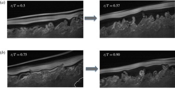
Figure 9(a) compares images of the ramp boundary layer over the straight section of the ramp,
 $0.6\leqslant x/L\leqslant 1.0$
, at the instant of airfoil plasma initiation (
 $t/T=0.5$
) and after the airfoil suction surface flow has reattached (
 $t/T=0.57$
). The effect of the increase in boundary layer thickness associated with the more severe APG is apparent. In figure 9(b), the ramp boundary layer is shown over the same spatial extent at the instant the airfoil plasma is extinguished (
 $t/T=0.75$
). At this instant, the airfoil flow is still attached and the ramp boundary layer shows a region of separated flow near the aft end of the ramp as a consequence of exposure to the more severe APG. In the photo to the right (
 $t/T=0.9$
), the airfoil flow has now separated and the ramp boundary layer has thinned and undergone reattachment.
Sample images of the ramp boundary layer flow for
 $0.6\leqslant x/L\leqslant 1.0$
during the time intervals for (a) airfoil flow reattachment and (b) airfoil flow separation.

The actuation signal shown previously in figure 6 is supplied to two separate two-channel Crown XTi4000 power amplifiers. The amplified signals are passed through a series of two
 $1~\unicode[STIX]{x03A9}$
resistors to limit the current. The signal is then split and sent through two 1 : 360 transformers. The transformers produce two high-voltage a.c. output signals that are
 $180^{\circ }$
out of phase. One signal is supplied to the exposed electrode and the other to the covered electrode of the plasma actuator on the leading edge of the airfoil. This gives rise to a 15 kV peak-to-peak version of the signal shown in figure 6. This applied voltage was found to be sufficient to produce a body force capable of consistently reattaching the airfoil suction surface flow within 60 ms of plasma initiation.
2.4 Ramp time-mean and phase-averaged pressure distributions
In this paper, flow quantities
 $g(\boldsymbol{x},t)$
are expressed in terms of a triple decomposition,
 $$\begin{eqnarray}g(\boldsymbol{x},t)=\overline{g}(\boldsymbol{x})+\tilde{g}(\boldsymbol{x},t)+g^{\prime }(\boldsymbol{x},t).\end{eqnarray}$$
In the above relation,
 $\overline{g}(\boldsymbol{x})$
is the time-averaged component,
 $\tilde{g}(\boldsymbol{x},t)$
is the phase-averaged coherent fluctuating component associated with the imposed unsteady pressure gradient cycle and
 $g^{\prime }(\boldsymbol{x},t)$
is the phase incoherent random turbulent component.
The phase average is given by
 $$\begin{eqnarray}\langle g(\boldsymbol{x},t)\rangle \equiv \lim _{N\rightarrow \infty }\frac{1}{N}\mathop{\sum }_{n=1}^{N}g(\boldsymbol{x},t+nT),\end{eqnarray}$$
where
 $T$
is the period of the unsteady cycle shown previously in figure 6 and
 $N$
is the number of unsteady cycles used for the phase average. It follows that
 $$\begin{eqnarray}\displaystyle & \tilde{g}(\boldsymbol{x},t)=\langle g(\boldsymbol{x},t)\rangle -\overline{g}(\boldsymbol{x}), & \displaystyle\end{eqnarray}$$
 $$\begin{eqnarray}\displaystyle & g(\boldsymbol{x},t)=\langle g(\boldsymbol{x},t)\rangle +g^{\prime }(\boldsymbol{x}). & \displaystyle\end{eqnarray}$$
A total of 34 static surface pressure taps placed along the centreline of the convex ramp model were used to measure the imposed streamwise surface pressure distribution for the two conditions of fully attached (plasma on) and separated (plasma off) airfoil flow. In essence, these ramp surface pressure distributions describe the two extremes of the temporal ramp surface pressure variation. The pressure taps were connected via internal tubing to a 48-port Scanivalve SSS-48C9 system. The Scanivalve housed a differential pressure transducer (model number PDCR23D) and signal conditioner (Scanivalve Corp. SCSG2) which were used to measure the time-averaged surface pressure distribution along the ramp section. The surface pressure coefficient is defined as
 $C_{p}\equiv (P-P_{\infty })/(P_{0}-P_{\infty })$
, where
 $P$
is the static pressure measured at the wall pressure tap, and
 $P_{0}$
and
 $P_{\infty }$
are the free-stream total and static pressures respectively, as measured by a Pitot static probe suspended from the tunnel ceiling 32 mm upstream of the ramp section. The measured pressure coefficients have a
 $\pm 2.8\,\%$
relative uncertainty at 20 : 1 odds. Spanwise-oriented arrays of static pressure taps at selected streamwise locations confirmed the two-dimensionality of the imposed surface pressure distributions in the mean to within
 $\pm 3\%$
.
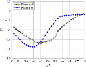
Figure 10 shows the time-averaged surface pressure coefficient distribution over the ramp with the airfoil plasma flow control both off and on. The
 $C_{p}$
distribution is presented as a function of
 $x/L$
, where
 $x$
is the streamwise spatial coordinate along the ramp surface and
 $L=37.54$
cm (14.78 in.) is the total length of the ramp (figure 1
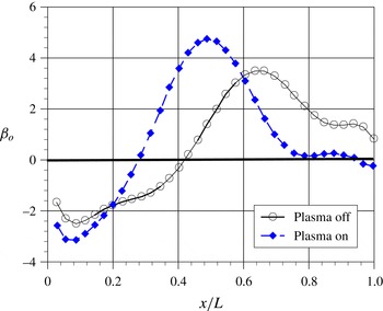
b). Figure 11 shows the corresponding non-dimensional pressure gradient parameter, defined as
 $\unicode[STIX]{x1D6FD}\equiv (\unicode[STIX]{x1D6FF}^{\ast }/\unicode[STIX]{x1D70F}_{w})_{o}\,\text{d}P/\text{d}x$
, where the subscript
 $o$
denotes that the displacement thickness,
 $\unicode[STIX]{x1D6FF}^{\ast }$
, and wall-shear stress,
 $\unicode[STIX]{x1D70F}_{w}$
, are evaluated at the origin of the convex ramp section (
 $x=0$
). The values of
 $\unicode[STIX]{x1D6FD}_{o}$
were calculated from the
 $C_{p}$
data shown in figure 10. It is important to note that the
 $\unicode[STIX]{x1D6FD}_{o}$
values shown in figure 11 are based on initial values of
 $\unicode[STIX]{x1D6FF}^{\ast }$
and
 $\unicode[STIX]{x1D70F}_{w}$
and serve only to provide a comparison of the non-dimensional pressure gradients for the plasma-on and plasma-off cases. Values of
 $\unicode[STIX]{x1D6FD}$
on the ramp surface will be much larger under the influence of the APG since
 $\unicode[STIX]{x1D6FF}^{\ast }$
grows,
 $\unicode[STIX]{x1D70F}_{w}$
is diminished and
 $\unicode[STIX]{x1D6FD}(x/L)=\unicode[STIX]{x1D6FD}_{o}[(\unicode[STIX]{x1D6FF}^{\ast }(x/L)/\unicode[STIX]{x1D6FF}_{o}^{\ast })(\unicode[STIX]{x1D70F}_{Wo}/\unicode[STIX]{x1D70F}_{W})]$
. For example, at
 $x/L=0.72$
,
 $\unicode[STIX]{x1D6FD}/\unicode[STIX]{x1D6FD}_{o}=3.5$
for the plasma-off case and
 $\unicode[STIX]{x1D6FD}/\unicode[STIX]{x1D6FD}_{o}=12$
for the plasma-on case.
Measured mean convex ramp surface pressure distributions for the airfoil plasma-on and plasma-off cases.

Non-dimensional streamwise pressure gradient,
 $\unicode[STIX]{x1D6FD}_{o}\equiv (\unicode[STIX]{x1D6FF}^{\ast }/\unicode[STIX]{x1D70F}_{w})_{o}\,\text{d}P/\text{d}x$
, on the convex ramp for airfoil plasma-on and plasma-off cases.

Figure 11 shows that in the absence of airfoil leading edge plasma flow control (i.e. with the airfoil flow separated), a favourable pressure gradient (
 $\unicode[STIX]{x1D6FD}<0$
) exists over approximately the first 40 % of the ramp section followed by an APG over the reminder of the ramp. The APG peaks near
 $x/L=0.65$
and is subsequently reduced over the last 35 % of the ramp section. Laser Doppler velocimetry (LDV) measurements (to be presented) will show that in this case, the APG turbulent boundary layer remains attached to the ramp surface, but near a state of incipient separation.
With the airfoil plasma control on, the ramp surface pressure results show that, after an initially favourable pressure gradient over the first 24 % of the ramp section, there is a larger APG over the remainder of the ramp, with the peak value occurring near
 $x/L=0.5$
. A plateau of constant
 $C_{p}$
values for
 $x/L>0.9$
shown in figure 10 is associated with turbulent boundary layer separation from the ramp surface.
In order to measure the effect of the airfoil plasma actuation on the unsteady ramp surface pressure, three high-frequency-response Endevco 8507C-1 piezoresistive pressure transducers were flush mounted on the ramp centreline at the representative streamwise locations of
 $x/L=0.67$
, 0.80 and 0.94. In this manner, two of the transducers were located upstream of the steady-state plasma-on separation location at
 $x/L=0.90$
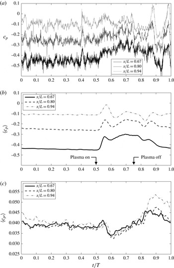
, with the third located just downstream. Signals from the three pressure transducers were recorded at a sample frequency of 20 kHz and anti-alias filtered at a frequency of 10 kHz using an Endevco model 136 signal conditioner. Figure 12(a) shows a single representative sample trace of the instantaneous surface pressure coefficient for each of the three streamwise locations on the ramp surface during the unsteady cycle.
Figure 12(b) shows the corresponding phase-averaged wall pressure coefficient,
 $\langle c_{P}\rangle$
, computed from (2.2) with
 $N=250$
unsteady cycles, which was found to be sufficient to produce a fully converged phase average. Shortly after the onset of plasma actuation at
 $t/T=0.5$
, each of the phase-averaged pressure coefficients shows a rapid increase towards a peak value of
 $\langle c_{P}\rangle$
followed by a shallow local minimum. Inspection of figure 12(b) reveals that the
 $\langle c_{P}\rangle$
peak convects downstream at speed
 $U_{c}/U_{\infty }=0.95\pm 0.02$
. The sudden shift to higher values of
 $\langle c_{P}\rangle$
is associated with the plasma flow control reattaching the flow on the suspended airfoil, as depicted previously in figure 7. The peak and local minimum shown in the traces in figure 12(b) represent the transient airfoil wake passage over the ramp as the airfoil flow undergoes reattachment. Following this initial overshoot, the values of
 $\langle c_{P}\rangle$
gradually increase during the interval
 $0.6\leqslant t/T\leqslant 0.70$
and the boundary layer undergoes separation on the most downstream portion of the ramp section (as demonstrated later in § 3). The pressure signal at
 $x/L=0.67$
(the location farthest upstream of the separation) shows the largest change in magnitude throughout the unsteady cycle. The pressure signal for the transducer just downstream of the unsteady separation,
 $x/L=0.94$
, shows comparatively little change in the magnitude for the unsteady cycle.
(a) Instantaneous pressure coefficients on the ramp for one unsteady cycle. (b) Phase-averaged pressure coefficient on the ramp for one unsteady cycle. (c) Phase-averaged turbulent root mean square (r.m.s.) pressure coefficient for one unsteady cycle.

The airfoil plasma is extinguished at
 $t/T=0.75$
, and this initiates a gradual reduction in values of
 $\langle c_{P}\rangle$
as the airfoil flow separation process commences. A local minimum followed by a peak in
 $\langle c_{P}\rangle$
shown in the traces for
 $t/T>0.8$
is a result of the flow separating from the airfoil section after the airfoil plasma flow control has been turned off during the unsteady cycle. The convection speed for this
 $\langle c_{P}\rangle$
peak is reduced to
 $U_{c}/U_{\infty }\approx 0.31$
due to the imposed APG. Figure 12(c) presents the phase-averaged r.m.s. pressure coefficient,
 $\langle c_{P\,rms}\rangle$
, for the unsteady cycle. After passage of the airfoil wake transient,
 $\langle c_{P\,rms}\rangle$
is reduced on the ramp. Significant increases are noted after the plasma is extinguished, and this is largest for
 $x/L=0.94$
and is associated with the unsteady reattachment of the separated ramp flow. Not only do the largest values of
 $\langle c_{P\,rms}\rangle$
occur for
 $x/L=0.94$
, but this location also requires the largest time interval to relax back to nominal attached flow values (which appears to be complete near
 $t/T=0.3$
).
3 Characterization of the convex ramp turbulent boundary layer
3.1 Ramp boundary layer mean velocity and turbulence intensity
Local wall-normal profiles of two-component mean and fluctuating velocity along the centreline of the convex ramp section were obtained non-intrusively using a Dantec Dynamics Fiber Flow LDV system. The fibre optic LDV system was operated in
 $180^{\circ }$
backscatter mode. The boundary layer flow was seeded with olive oil particles of nominally
 $1~\unicode[STIX]{x03BC}\text{m}$
diameter which were introduced upstream of the wind tunnel inlet with a liquid droplet seeding generator. The LDV probe volume was traversed locally normal to the convex ramp surface over a range of
 $x/L$
locations using a three-axis Aerotech traverse system and Unidex 11 controller. The probe measurement volume had a maximum wall-normal dimension of 0.35 mm (0.0138 in), which set the effective spatial resolution of the boundary layer measurements. The true
 $y$
location relative to the surface was established via a separate optics-based calibration procedure.
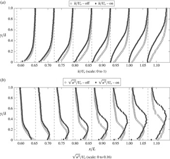
Prior to characterizing the unsteady aspects of the APG turbulent boundary layer, consideration is first given to the time-mean boundary layer behaviour for both the imposed plasma-on and plasma-off pressure gradients shown previously in § 2. Figure 13 documents the spatial evolution of streamwise mean velocity and streamwise-component turbulence intensity profiles along the ramp for both the less severe (airfoil plasma-off) and more severe (airfoil plasma-on) APG cases. Each profile is made non-dimensional by the local external velocity,
 $U_{e}(x/L)$
, and the wall-normal coordinate is scaled by the local boundary layer thickness,
 $\unicode[STIX]{x1D6FF}(x/L)$
. It is apparent from figure 13 that the ramp boundary layer flow is significantly influenced by the variation in the imposed APG.
The mean velocity profiles for the plasma-off case show that the boundary layer remains attached at all locations on the ramp section. This was also confirmed with surface oil flow visualization (not shown). In contrast, for the plasma-on case, the velocity defect is observed to be much larger, and time-averaged near-wall reversed flow occurs at downstream locations on the ramp section (
 $x/L>0.9$
). This aspect will be considered further in § 3.2.
The corresponding turbulence intensity profiles show that in both APG cases, the location of peak r.m.s. turbulence shifts away from the wall as the flow evolves in
 $x/L$
. However, both the magnitude of the peak turbulence intensity and its distance from the wall increase significantly with the severity of the imposed APG, as does the reduction in near-wall turbulence levels. In contrast to the ZPG turbulent boundary layer, the turbulence peak is broader, is of greater amplitude and occurs much farther away from the wall. The data in figure 13 are consistent with the results of Krogstad & Skåre (Reference Krogstad and Skåre1995), Shah et al. (Reference Shah, Laval and Stanislas2009) and Monty, Harun & Marusic (Reference Monty, Harun and Marusic2011), where it was also found that r.m.s. velocity fluctuation profiles from APG turbulent boundary layers showed a turbulence peak that moved away from the wall as the magnitude of the APG grew.
The LDV measured (a) time-mean streamwise velocity and (b) turbulence intensity profiles along the convex ramp for the plasma-on and plasma-off cases.

3.2 Transient response of the ramp boundary layer
In order to initially characterize the transient response of the ramp turbulent boundary layer to the imposed unsteady pressure gradient, an array of six Auspex straight hot-wire probes was utilized. The sampling frequency was 13 kHz and the probes were separated in the wall-normal direction by
 $\unicode[STIX]{x0394}y=8$
mm (
 $\unicode[STIX]{x0394}y/\unicode[STIX]{x1D6FF}=0.21$
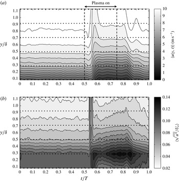
). As a representative example, figure 14(a) presents a contour plot of the phase-averaged velocity based on 250 unsteady pressure gradient cycles with the hot-wire rake located at a streamwise location of
 $x/L=0.80$
, which is upstream of any reverse flow that takes place during the unsteady cycle (and which obviously cannot be detected by the hot-wire array). The time interval associated with airfoil plasma flow control is indicated in the figure.
(a) Temporal variation in phase-averaged streamwise velocity at
 $x/L=0.8$
(dotted horizontal lines indicate probe positions). (b) Temporal variation in phase-averaged turbulence intensity at
 $x/L=0.8$
(dotted horizontal lines indicate probe positions).

It is apparent from figure 14(a) that the ramp boundary layer momentum defect grows very rapidly in response to the increase in APG that commences at
 $t/T=0.5$
. It should be noted that for fixed
 $y/\unicode[STIX]{x1D6FF}$
, there is an initial increase in phase-averaged velocity near
 $t/T=0.53$
followed by a large reduction. This transient behaviour is associated with the passage of the airfoil wake as part of the airfoil flow attachment process (see figure 7). After the plasma is extinguished at
 $t/T=0.75$
, the phase-averaged velocity contours remain constant until approximately
 $t/T=0.8$
, and reference to figure 8 indicates that this delay is associated with the time interval required for the airfoil flow separation process to commence. Figure 14(a) shows a marked reduction in the velocity defect commencing near
 $t/T=0.8$
. The airfoil flow is fully separated by
 $t/T=0.9$
, and at the same time figure 14(a) shows a transient increase in velocity defect which appears to be associated with the ramp boundary layer reattachment process.
Figure 14(b) presents the corresponding temporal evolution of the phase-averaged streamwise-component turbulence intensity at
 $x/L=0.8$
. The sharp peak near
 $t/T=0.55$
is due to the velocity fluctuations in the outer flow associated with the passage of the transient airfoil wake and its jitter. Shortly after the wake passage, the boundary layer peak turbulence intensity rapidly shifts away from the wall and peak values are found near
 $y/\unicode[STIX]{x1D6FF}=0.3$
. This is consistent with the turbulence intensity profiles shown in figure 13. Conditional LDV measurements to be presented in the next section will show that this is associated with the development of an embedded shear layer within the unsteady APG boundary layer. During this portion of the unsteady cycle in the interval
 $0.6\leqslant t/T\leqslant 0.85$
, the turbulence intensity continually increases to reach a maximum value before onset of the reattachment process.
A more extensive set of phase-averaged measurements of the unsteady boundary layer were performed non-intrusively using LDV. At each spatial location,
 $10^{6}$
samples were acquired for each velocity component. Due to the LDV data rate dependence on the particle crossings (9–12 kHz), a bin averaging technique was used to determine the phase intervals of the LDV data (see Sonnenberger, Graichen & Erk Reference Sonnenberger, Graichen and Erk2000). In this method, the unsteady period,
 $T$
, is subdivided into 180 elementary intervals referred to as phase ‘bins’, of width
 $\unicode[STIX]{x0394}\unicode[STIX]{x1D719}=2^{\circ }$
, and the centre of each bin is denoted by a phase angle,
 $\unicode[STIX]{x1D719}$
, in the unsteady cycle. The estimate of the phase-averaged value from bin averaging the samples of a velocity component is given by
 $$\begin{eqnarray}\langle u(\unicode[STIX]{x1D719})\rangle =\frac{1}{N(\unicode[STIX]{x1D719})}\mathop{\sum }_{n=1}^{N(\unicode[STIX]{x1D719})}u_{n}(\unicode[STIX]{x1D719}),\end{eqnarray}$$
where
 $N(\unicode[STIX]{x1D719})\geqslant 5000$
denotes the number of samples in each phase bin. The phase-averaged r.m.s. of the velocity component is estimated by
 $$\begin{eqnarray}\left\langle \sqrt{u^{\prime 2}(\unicode[STIX]{x1D719})}\right\rangle =\sqrt{\frac{1}{N(\unicode[STIX]{x1D719})-1}\mathop{\sum }_{n=1}^{N(\unicode[STIX]{x1D719})}(u_{n}(\unicode[STIX]{x1D719})-\langle u(\unicode[STIX]{x1D719})\rangle )^{2}}.\end{eqnarray}$$
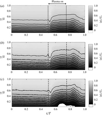
Figure 15 presents contour plots illustrating the temporal evolution of the phase-averaged velocity,
 $\langle u/U_{e}\rangle$
, during the unsteady cycle for ramp locations of
 $x/L=0.86$
, 0.93 and 1.0. The time interval for plasma flow control on the airfoil is again denoted in the figure by vertical dashed lines. Key features regarding the response of the turbulent boundary layer to the imposed unsteady pressure gradient at locations both upstream and downstream of the separation on the aft portion of the ramp section are shown. In each case, the wall-normal coordinate is normalized by the local boundary layer thickness,
 $\unicode[STIX]{x1D6FF}(x/L)$
. After the airfoil flow has reattached near
 $t/T=0.55$
, the velocity contour levels at fixed
 $y/\unicode[STIX]{x1D6FF}$
drop significantly, which is a manifestation of the growth of the momentum defect in the normalized wall coordinate. It should be noted that at the location
 $x/L=1.0$
, a region of phase-averaged reverse flow is measured near the wall for
 $0.65\leqslant t/T\leqslant 0.85$
, as indicated by the white contour region. Upon termination of the plasma at
 $t/T=0.75$
, the velocity contour levels increase at fixed
 $y/\unicode[STIX]{x1D6FF}$
as the boundary layer momentum defect is reduced during the reattachment process from
 $t/T=0.85$
to
 $1.0$
. Careful inspection of figure 15 shows that the boundary layer phase-averaged velocity continues to recover from the previous unsteady separation cycle until approximately
 $t/T=0.2$
.
Contour plots of the temporal evolution of ramp boundary layer phase-averaged streamwise velocity,
 $\langle u/U_{e}\rangle$
, based on LDV measurement: (a)
 $x/L=0.86$
, (b)
 $x/L=0.93$
, (c)
 $x/L=1.0$
.

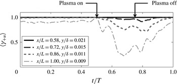
Figure 16 presents the fraction of time the phase-averaged near-wall flow is in the streamwise direction,
 $\langle \unicode[STIX]{x1D6FE}_{+U}\rangle$
, for a representative range of
 $x/L$
locations along the ramp section. In each case, the LDV probe volume was placed as close to the wall as possible. The indicated
 $y/\unicode[STIX]{x1D6FF}$
locations in figure 16 differ due to the growth in the local boundary layer thickness,
 $\unicode[STIX]{x1D6FF}(x,t)$
. For the period
 $0\leqslant t/T\leqslant 0.5$
(airfoil plasma off), no phase-averaged reverse flow is detected for the locations
 $x/L=0.58$
, 0.72 and 0.86 since
 $\langle \unicode[STIX]{x1D6FE}_{+U}\rangle =1$
. During the same time period, the flow at
 $x/L=1$
shows
 $\langle \unicode[STIX]{x1D6FE}_{+U}\rangle =0.9$
, which indicates that the boundary layer at the farthest downstream ramp location is in a state of incipient detachment for the comparatively mild APG.
Upon application of the more severe APG for
 $0.5\leqslant t/T\leqslant 0.75$
, the most upstream location,
 $x/L=0.58$
, still indicates no phase-averaged reverse flow throughout the unsteady cycle. At
 $x/L=0.72$
, phase-averaged reverse flow for the same interval occurs not more than 8 % of the time. In contrast, the measurements at
 $x/L=0.86$
in the interval
 $0.65\leqslant t/T\leqslant 0.85$
show that phase-averaged reverse flow is detected approximately 20 % of the time (
 $\langle \unicode[STIX]{x1D6FE}_{+u}\rangle \approx 0.80$
), which is defined as a state of intermittent transitory detachment (see Simpson Reference Simpson1996). At
 $x/L=1.0$
, in the interval
 $0.62\leqslant t/T\leqslant 0.82$
, reverse flow is detected more than 50 % of the time, which is indicative of the existence of a separated boundary layer (Simpson Reference Simpson1996). It may be noted that the return to a state of incipient separation at
 $x/L=1.0$
takes approximately twice as long as the onset of flow separation.
Fraction of time the phase-averaged near-wall flow moves in the streamwise direction,
 $\left\langle \unicode[STIX]{x1D6FE}_{+u}\right\rangle$
, for selected
 $x/L$
locations along the ramp.

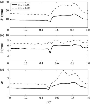
Variation of phase-averaged turbulent boundary layer displacement thickness, momentum thickness and shape factor with
 $t/T$
for locations of
 $x/L=0.86$
and 1.0.

The phase-averaged velocity profiles measured on the ramp section were used to calculate the temporal variation of global boundary layer quantities throughout the unsteady cycle. As an example, figure 17 shows the temporal variation of the boundary layer displacement thickness,
 $\unicode[STIX]{x1D6FF}^{\ast }$
, the momentum thickness,
 $\unicode[STIX]{x1D703}$
, and the shape factor,
 $H$
, with
 $t/T$
for representative locations of
 $x/L=0.86$
and
 $x/L=1.0$
. After plasma initiation, the displacement thickness shows a brief reduction near
 $t/T=0.52$
, which is associated with the convection of the increased wake region behind the airfoil as a result of the unsteady forcing that reattaches the leading edge (see figure 7). The displacement thickness subsequently increases to reach a maximum value near
 $t/T=0.82$
just before the boundary layer reattachment process begins on the ramp section. After application of the increased APG, the momentum thickness at
 $x/L=0.86$
increases by 26 % to reach a nearly constant value for the separated part of the cycle. The increase in
 $\unicode[STIX]{x1D703}$
at
 $x/L=1.0$
is observed to be much smaller. The shape factor for the
 $x/L=0.86$
location increases from an initial value near
 $H=1.8$
to a peak value of 2.53 near
 $t/T=0.8$
. At
 $x/L=1.0$
, the velocity profile shape factor shifts from a value of 2.35 during the attached portion of the cycle to a maximum value of 3.9 at
 $t/T=0.68$
, when the boundary layer profile shows the largest degree of reversed flow near the wall. As a basis for comparison, it should be recalled that for near-equilibrium flows consistent with Cole’s mean velocity profile, intermittent transitory detachment occurs near
 $H=2.7$
.
With the basic character of the unsteady ramp boundary layer documented, the next section is focused on the influence of the imposed unsteady pressure gradient on the nature of the coherent structure in the ramp turbulent boundary layer. This is explored via a series of conditional measurements.
4 Conditional boundary layer measurements
It is well known that Reynolds stress and turbulence production is, in large part, a result of coherent motions within the turbulent boundary layer (e.g. Kovasznay Reference Kovasznay1970; Robinson Reference Robinson1991). Such events are often characterized as ejections of relatively low-speed fluid outward from the wall, and sweeps of high-speed fluid towards the wall. This section investigates the effect of the unsteady imposed APG on the character of these coherent near-wall events. The effect is documented using a series of conditional LDV measurements of the convex ramp unsteady turbulent boundary layer flow.
4.1 Application of the quadrant-splitting technique
Ejection and sweep events were quantified using the
 $u^{\prime }v^{\prime }$
quadrant-splitting (QS) technique initially developed and utilized by Wallace, Eckelmann & Brodkey (Reference Wallace, Eckelmann and Brodkey1972) and Willmarth & Lu (Reference Willmarth and Lu1972). Ejection events reside in the second quadrant (
 $u^{\prime }(t)<0$
,
 $v^{\prime }(t)>0$
), and are generally associated with both spanwise vortices that form the head of a vortical hairpin arch and streamwise-oriented near-wall vortices (see figure 13 of Robinson Reference Robinson1991). The fourth-quadrant (
 $u^{\prime }(t)>0,v^{\prime }(t)<0$
) motions are associated with the tilted neck elements of a vortical arch. Lu & Willmarth (Reference Lu and Willmarth1973) were the first to show that discrete second-quadrant (Q2) and fourth-quadrant (Q4) events are the primary contributors to the Reynolds stress production in a turbulent boundary layer.
In this study, the QS technique was implemented by using an identification (ID) function to determine those instants of time when
 $u^{\prime }(t)$
and
 $v^{\prime }(t)$
are in a given quadrant, and their product
 $u^{\prime }(t)v^{\prime }(t)$
exceeds a specified threshold level. The ID functions for quadrant 2 and quadrant 4 are respectively
 $$\begin{eqnarray}\displaystyle & \displaystyle \text{ID}_{Q2}(t,\unicode[STIX]{x1D6FC}_{q})=\left\{\begin{array}{@{}ll@{}}1\quad & \text{if }u^{\prime }(t)<0\text{ and }u^{\prime }(t)v^{\prime }(t)<-\unicode[STIX]{x1D6FC}_{q}\sqrt{\overline{u^{\prime 2}}}\sqrt{\overline{v^{\prime 2}}},\\ 0\quad & \text{otherwise},\end{array}\right. & \displaystyle\end{eqnarray}$$
 $$\begin{eqnarray}\displaystyle & \displaystyle \text{ID}_{Q4}(t,\unicode[STIX]{x1D6FC}_{q})=\left\{\begin{array}{@{}ll@{}}1\quad & \text{if }u^{\prime }(t)>0\text{ and }u^{\prime }(t)v^{\prime }(t)<-\unicode[STIX]{x1D6FC}_{q}\sqrt{\overline{u^{\prime 2}}}\sqrt{\overline{v^{\prime 2}}},\\ 0\quad & \text{otherwise},\end{array}\right. & \displaystyle\end{eqnarray}$$
where
 $\unicode[STIX]{x1D6FC}_{q}$
determines the size of the so-called ‘hyperbolic hole’ defined by the product of the r.m.s. values of
 $u^{\prime }$
and
 $v^{\prime }$
. Narasimha et al. (Reference Narasimha, Kumar, Prabhu and Kailas2010) found that the r.m.s. value is more appropriate than the mean Reynolds stress value for calculating the threshold since the fluctuations of
 $u^{\prime }(t)v^{\prime }(t)$
can be large multiples of the mean as the flow approaches separation. Only a single event is counted when the ID function is satisfied for an unbroken sequence of temporal samples, and ID functions for Q1 and Q3 events were similarly defined.
The relative contribution to the Reynolds stress from the various quadrant motions was determined from
 $$\begin{eqnarray}\frac{\overline{u^{\prime }v_{i}^{\prime }}(\unicode[STIX]{x1D6FC}_{q})}{\overline{u^{\prime }v^{\prime }}}=\frac{1}{\overline{u^{\prime }v^{\prime }}}\lim _{T\rightarrow \infty }\frac{1}{T}\int _{0}^{T}u^{\prime }(t)v^{\prime }(t)\text{ID}_{Q_{i}}(t,\unicode[STIX]{x1D6FC}_{q})\,\text{d}t,\end{eqnarray}$$
where the subscript
 $i$
refers to the
 $i\text{th}$
quadrant. The contribution to
 $\overline{u^{\prime }v^{\prime }}$
from within the hyperbolic hole region was obtained from the relation
 $$\begin{eqnarray}\frac{\overline{u^{\prime }v^{\prime }}_{H}(\unicode[STIX]{x1D6FC}_{q})}{\overline{u^{\prime }v^{\prime }}}=\frac{1}{\overline{u^{\prime }v^{\prime }}}\lim _{T\rightarrow \infty }\frac{1}{T}\int _{0}^{T}u^{\prime }(t)v^{\prime }(t)\text{ID}_{H}(t,\unicode[STIX]{x1D6FC}_{q})\,\text{d}t,\end{eqnarray}$$
where the ID function for the hyperbolic hole is defined as
 $$\begin{eqnarray}\text{ID}_{H}(t,\unicode[STIX]{x1D6FC}_{q})=\left\{\begin{array}{@{}ll@{}}1\quad & \text{if }|u^{\prime }(t)v^{\prime }(t)|<\unicode[STIX]{x1D6FC}_{q}\sqrt{\overline{u^{2}}}\sqrt{\overline{v^{2}}},\\ 0\quad & \text{otherwise}.\end{array}\right.\end{eqnarray}$$
The contributions from the four quadrants and the hole region are all functions of the threshold level,
 $\unicode[STIX]{x1D6FC}_{q}$
, and it follows that
 $$\begin{eqnarray}\mathop{\sum }_{i=1}^{4}\frac{\overline{u^{\prime }v_{i}^{\prime }}(\unicode[STIX]{x1D6FC}_{q})}{\overline{u^{\prime }v^{\prime }}}+\frac{\overline{u^{\prime }v_{H}^{\prime }}(\unicode[STIX]{x1D6FC}_{q})}{\overline{u^{\prime }v^{\prime }}}=1.\end{eqnarray}$$
For validation purposes and to form a basis for comparison with the APG convex ramp boundary layer, the QS technique was first applied to the ZPG turbulent boundary layer on the flat plate just upstream of the convex ramp section. The QS results are based on
 $10^{6}$
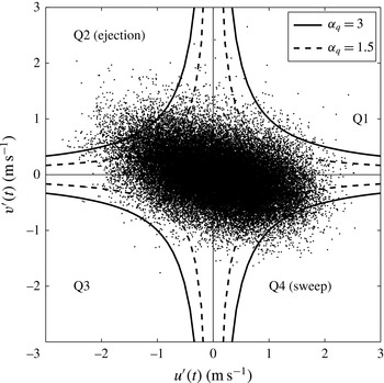
LDV velocity measurements obtained at each spatial location. Figure 18 shows the
 $u^{\prime }(t)$
and
 $v^{\prime }(t)$
velocity components measured by LDV on the boundary layer development plate at a wall-normal location of
 $y^{+}=105$
. The figure shows the quadrants in the
 $u^{\prime }v^{\prime }$
plane and also sketches sample hyperbolic holes defined for
 $\unicode[STIX]{x1D6FC}_{q}=1.5$
and
 $\unicode[STIX]{x1D6FC}_{q}=3$
. This figure clearly shows the preference for the quadrants 2 and 4 Reynolds stress-producing events, which is typical of a ZPG turbulent boundary layer.
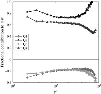
Figure 19 presents inner variable scaled profiles of the fractional contribution of each quadrant to
 $\overline{u^{\prime }v^{\prime }}$
in the approach ZPG turbulent boundary layer with
 $\unicode[STIX]{x1D6FC}_{q}=0$
. These results are in very good agreement with similar measurements presented in figure 4 of Wallace et al. (Reference Wallace, Eckelmann and Brodkey1972). For example, at
 $y^{+}=36$
, the Q2 and Q4 events account for 81 % and 66 % respectively of the mean Reynolds stress (with the balance associated with Q1 and Q3 events), in good agreement with both Wallace et al. (Reference Wallace, Eckelmann and Brodkey1972) and Lu & Willmarth (Reference Lu and Willmarth1973).
The
 $u^{\prime }(t)$
and
 $v^{\prime }(t)$
velocity components measured near the end of the flat boundary layer development plate (
 $x/L=-0.085$
) at the wall-normal location of
 $y^{+}=105$
. Also shown are the hyperbolic holes for
 $\unicode[STIX]{x1D6FC}_{q}=1.5$
and 3.0.

Sample profiles of the fractional contribution to
 $-\overline{u^{\prime }v^{\prime }}$
from each quadrant (
 $\unicode[STIX]{x1D6FC}_{q}=0$
) in the ZPG turbulent boundary layer near the end of the flat boundary layer development plate (
 $x/L=-0.085$
).

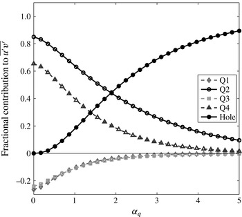
Fractional contribution of each quadrant to
 $\overline{u^{\prime }v^{\prime }}$
as a function of the hyperbolic hole size,
 $\unicode[STIX]{x1D6FC}_{q}\sqrt{\overline{u^{\prime 2}}}\sqrt{\overline{v^{\prime 2}}}$
, at a sample wall-normal location of
 $y^{+}=36$
in the ZPG boundary layer at
 $x/L=-0.085$
.

Figure 20 shows the fractional contribution of each quadrant as a function of the hole size,
 $\unicode[STIX]{x1D6FC}_{q}$
, at the same wall-normal location of
 $y^{+}=36$
for the ZPG boundary layer. For a hole size of
 $\unicode[STIX]{x1D6FC}_{q}=4$
, which corresponds to a threshold level of 12 times the measured Reynolds stress, the Q2 events still account for 16 % of the contributions to
 $-\overline{u^{\prime }v^{\prime }}$
. These results are consistent with the measurements presented in figure 11 of Lu & Willmarth (Reference Lu and Willmarth1973) and further confirm the importance of the strong Q2 ejection events in the ZPG turbulent boundary layer.
4.2 Effect of APG on ejection and sweep events
It is known that the imposition of a streamwise pressure gradient influences the dynamic process of turbulence production in the boundary layer. For example, Krogstad & Skåre (Reference Krogstad and Skåre1995) showed that the APG turbulent boundary layer is dominated by strong Q4 sweep events, with Q2 ejection events nearly absent in the near-wall region. In stark contrast, Bourassa & Thomas (Reference Bourassa and Thomas2009) showed that for a favourable pressure gradient large enough to cause relaminarization, Q4 sweep events are largely eliminated, while infrequent but larger-amplitude near-wall Q2 ejection events still occur.
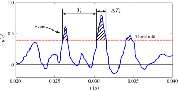
Schematic showing quadrant event duration,
 $\unicode[STIX]{x0394}T_{i}$
, and time interval between events,
 $T_{i}$
.

Prior to examination of the unsteady APG turbulent boundary layer, a representative comparison is first made between QS measurements for the ZPG approach boundary layer flow at
 $x/L=-0.085$
and the APG flow on the
 $25^{\circ }$
ramp at
 $x/L=0.93$
with the plasma off and the ramp turbulent boundary layer attached. In particular, the average time between events occurring in the
 $i\text{th}$
quadrant,
 $\overline{T_{i}^{\ast }}$
, which is defined as the time between consecutive upward or downward crossings of the
 $u^{\prime }v^{\prime }$
time series past the specified threshold level, and the duration of those events,
 $\overline{\unicode[STIX]{x0394}T_{i}^{\ast }}$
, defined as the mean time between consecutive upward and downward crossings of the threshold level, are examined. These time intervals are defined in the schematic shown in figure 21. In order to remove the effect of convective time-scale differences between the ZPG and APG flow fields, following Antonia & Krogstad (Reference Antonia and Krogstad1992), these characteristic mean times are presented and compared in scaled form
 $\overline{T_{i}^{\ast }}\equiv \bar{T}_{i}\,U_{e}/\unicode[STIX]{x1D6FF}$
and
 $\overline{\unicode[STIX]{x0394}T_{i}^{\ast }}\equiv \overline{\unicode[STIX]{x0394}T_{i}}\,U_{e}/\unicode[STIX]{x1D6FF}$
. Also presented is the time-scale ratio,
 $\overline{\unicode[STIX]{x0394}T_{i}}/\overline{T_{i}}$
(an approach used by Krogstad & Skåre (Reference Krogstad and Skåre1995)), which is independent of convective speed. Large values of this ratio are associated with frequent and/or long-duration events that are expected to be the most dynamically significant. Conversely, small values of
 $\overline{\unicode[STIX]{x0394}T_{i}}/\overline{T_{i}}$
correspond to comparatively infrequent and/or short duration events, which would not be as dynamically important.
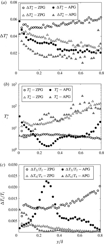
Figure 22 compares profiles of
 $\unicode[STIX]{x0394}\overline{T}_{2}^{\ast },\overline{T}_{2}^{\ast },\unicode[STIX]{x0394}\overline{T}_{4}^{\ast }$
and
 $\overline{T}_{4}^{\ast }$
as well as the ratios
 $\unicode[STIX]{x0394}\overline{T}_{2}/\overline{T}_{2}$
and
 $\unicode[STIX]{x0394}\overline{T}_{4}/\overline{T}_{4}$
for the ZPG and APG turbulent boundary layers at a threshold level of
 $\unicode[STIX]{x1D6FC}_{q}=4$
where the QS technique captures only the strongest events.
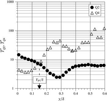
Figure 22(a) shows that for both ZPG and APG cases, strong Q2 events are of longer duration than strong Q4 events over the entire boundary layer. Furthermore, ZPG Q2 and Q4 events are of longer duration that the corresponding events in the APG flow with the exception of very near the wall where they become comparable.
Figure 22(b) shows that in the ZPG boundary layer, Q2 events are more frequent than Q4 events at all locations within the boundary layer. In contrast, for the APG case, Q4 events are more frequent than Q2 events for
 $y/\unicode[STIX]{x1D6FF}<0.12$
, with the disparity growing near the wall. For
 $y/\unicode[STIX]{x1D6FF}>0.12$
in the APG boundary layer, Q2 events become more frequent than Q4, with the disparity growing with increased distance from the wall.
Comparison of (a) mean duration
 $\unicode[STIX]{x0394}T_{i}^{\ast }$
and (b) mean time
 $T_{i}^{\ast }$
between Q2 and Q4 events, and (c) their ratio
 $\unicode[STIX]{x0394}T_{i}/T_{i}$
for ZPG and APG boundary layers with
 $\unicode[STIX]{x1D6FC}_{q}=4$
.

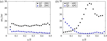
Comparison of fractional contribution of quadrant events to
 $\overline{u^{\prime }v^{\prime }}$
for ZPG and APG cases for strong events: (a) ZPG with
 $\unicode[STIX]{x1D6FC}_{q}=4$
; (b) APG with
 $\unicode[STIX]{x1D6FC}_{q}=4$
.

Figure 22(c) compares the ratios
 $\unicode[STIX]{x0394}\overline{T}_{2}/\overline{T}_{2}$
and
 $\unicode[STIX]{x0394}\overline{T}_{4}/\overline{T}_{4}$
for
 $\unicode[STIX]{x1D6FC}_{q}=4$
. For the ZPG boundary layer case,
 $\unicode[STIX]{x0394}\overline{T}_{2}/\overline{T}_{2}$
exceeds
 $\unicode[STIX]{x0394}\overline{T}_{4}/\overline{T}_{4}$
for all
 $y/\unicode[STIX]{x1D6FF}$
, and so the Q2 events are more dynamically significant than the Q4 events throughout the boundary layer. In contrast, for the APG boundary layer,
 $\unicode[STIX]{x0394}\overline{T}_{4}/\overline{T}_{4}$
exceeds
 $\unicode[STIX]{x0394}\overline{T}_{2}/\overline{T}_{2}$
for
 $y/\unicode[STIX]{x1D6FF}<0.12$
, indicating that strong Q4 motions dominate in the near-wall region. For
 $y/\unicode[STIX]{x1D6FF}>0.12$
, strong Q2 motions dominate, with a fairly localized peak in
 $\unicode[STIX]{x0394}\overline{T}_{2}/\overline{T}_{2}$
occurring near
 $y/\unicode[STIX]{x1D6FF}\approx 0.28$
. The implications of this regarding an embedded shear layer instability mechanism will be discussed in § 6.
Figure 23 compares the fractional contributions of the Q2 and Q4 events to the Reynolds stress,
 $\overline{u^{\prime }v_{1}^{\prime }}/\overline{u^{\prime }v^{\prime }}$
, for the ZPG and APG cases for strong events (
 $\unicode[STIX]{x1D6FC}_{q}=4$
). In the ZPG boundary layer, the contribution from strong ejection events (Q2) exceeds that from sweeps (Q4) over the entire lower half of the boundary layer. In contrast, for the APG boundary layer, strong Q4 sweep events become the dominant contributor in the near-wall region, accounting for nearly 25 % of the mean Reynolds stress near the wall, while the Q2 events account for less than 5 %. The Reynolds stress contributions from Q2 and Q4 events become comparable near
 $y/\unicode[STIX]{x1D6FF}=0.12$
, with ejection events becoming the dominant contributors farther from the wall. At
 $y/\unicode[STIX]{x1D6FF}=0.32$
, strong Q2 ejection events account for approximately 47 % of the mean Reynolds stress.
4.3 Quadrant-splitting measurements in the unsteady APG turbulent boundary layer
The QS technique described previously was modified in order to analyse the unsteady APG boundary layer. Bin (i.e. phase) averaging was used to determine the number of quadrant events that take place during the unsteady boundary layer cycle. At each measurement location, the QS technique was applied for
 $10^{6}$
unsteady boundary layer samples in the interval where the phase resolution was
 $\unicode[STIX]{x0394}\unicode[STIX]{x1D719}=2^{\circ }$
, resulting in phase estimates for 180 different phase bins. The numbers of Q2 and Q4 events detected for a particular phase value are given by
 $$\begin{eqnarray}\displaystyle \#\text{Q}2(\unicode[STIX]{x1D719})=\mathop{\sum }_{n=1}^{N(\unicode[STIX]{x1D719})}\text{ID}_{Q2}(\unicode[STIX]{x1D719},n), & & \displaystyle\end{eqnarray}$$
 $$\begin{eqnarray}\displaystyle \#\text{Q}4(\unicode[STIX]{x1D719})=\mathop{\sum }_{n=1}^{N(\unicode[STIX]{x1D719})}\text{ID}_{Q4}(\unicode[STIX]{x1D719},n), & & \displaystyle\end{eqnarray}$$
where the ID functions are now defined as
 $$\begin{eqnarray}\displaystyle \text{ID}_{Q2}(\unicode[STIX]{x1D719},n)=\left\{\begin{array}{@{}ll@{}}1\quad & \text{if }u_{n}^{\prime }(\unicode[STIX]{x1D719})<0\text{ and }u_{n}^{\prime }(\unicode[STIX]{x1D719})v_{n}^{\prime }(\unicode[STIX]{x1D719})<-\unicode[STIX]{x1D6FC}_{q}\left\langle \sqrt{u_{B}^{\prime 2}(\unicode[STIX]{x1D719})}\right\rangle \left\langle \sqrt{v_{B}^{\prime 2}(\unicode[STIX]{x1D719})}\right\rangle ,\\ 0\quad & \text{otherwise},\end{array}\right. & & \displaystyle\end{eqnarray}$$
 $$\begin{eqnarray}\displaystyle \text{ID}_{Q4}(\unicode[STIX]{x1D719},n)=\left\{\begin{array}{@{}ll@{}}1\quad & \text{if }u_{n}^{\prime }(\unicode[STIX]{x1D719})>0\text{ and }u_{n}^{\prime }(\unicode[STIX]{x1D719})v_{n}^{\prime }(\unicode[STIX]{x1D719})<-\unicode[STIX]{x1D6FC}_{q}\left\langle \sqrt{u_{B}^{\prime 2}(\unicode[STIX]{x1D719})}\right\rangle \left\langle \sqrt{v_{B}^{\prime 2}(\unicode[STIX]{x1D719})}\right\rangle ,\\ 0\quad & \text{otherwise}.\end{array}\right. & & \displaystyle \nonumber\\ \displaystyle & & \displaystyle\end{eqnarray}$$
It should be noted that the threshold level for the unsteady QS technique is referenced against the phase-averaged r.m.s. values of
 $u_{B}^{\prime }$
and
 $v_{B}^{\prime }$
, which denote velocity components for the given bin value. The remaining two quadrants are similarly defined. The hyperbolic hole with a value of
 $\unicode[STIX]{x1D6FC}_{q}=3$
was used to emphasize relatively strong quadrant events. However, conditional measurements using other threshold values (not shown here) showed that the event detection statistics were not overly sensitive to the hyperbolic hole size for a range of
 $\unicode[STIX]{x1D6FC}_{q}$
values.
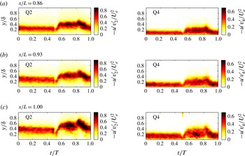
The dynamic behaviour of the Q2 and Q4 event contributions to the Reynolds stress for a threshold of
 $\unicode[STIX]{x1D6FC}_{q}=3$
is shown as a function of
 $t/T$
in the phase-averaged contour plots in figure 24. Results are shown for three representative locations on the ramp,
 $x/L=0.86$
, 0.93 and 1.0. During the plasma-off portion of the unsteady boundary layer cycle corresponding to
 $0\leqslant t/T\leqslant 0.5$
, the Q4 contribution to Reynolds stress is clearly dominant in the near-wall region. Peak values of the contribution to the Reynolds stress from Q2 events are relatively constant and lie above the Q4 contours at each streamwise location.
Contour plots of the temporal evolution of phase-averaged contributions to the scaled Reynolds stress
 $(\times 10^{-4})$
from Q2 and Q4 events at three locations along the ramp.

During the plasma-on portion of the cycle (
 $0.5<t/T\leqslant 0.75$
) for which the APG is more severe, the peak value of
 $\langle -u^{\prime }v_{Q2}^{\prime }/U_{e}^{2}\rangle$
increases in magnitude and also rather suddenly shifts farther away from the wall, and there is very little contribution to the Reynolds stress near the wall from Q2 ejection events. The peak values of
 $\langle -u^{\prime }v_{Q4}^{\prime }/U_{e}^{2}\rangle$
show an increase in magnitude and are spread throughout the lower portion of the boundary layer below the Q2 contours.
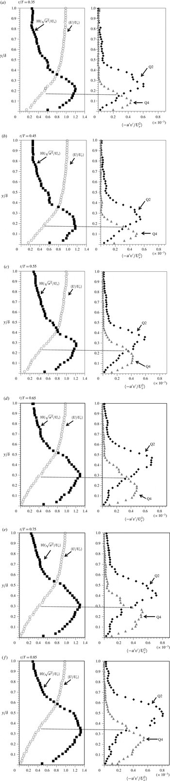
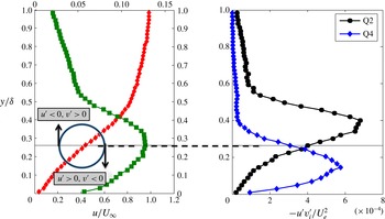
It is clear from this series of figures that the Q4 events are the dominant contributors to the Reynolds stress near the wall for the unsteady APG turbulent boundary layer. Perhaps most notable from figure 24 is that, regardless of position,
 $x/L$
, or phase,
 $t/T$
, contours of peak
 $\langle -u^{\prime }v_{Q2}^{\prime }/U_{e}^{2}\rangle$
always lie at
 $y/\unicode[STIX]{x1D6FF}$
locations just above contours of peak
 $\langle -u^{\prime }v_{Q4}^{\prime }/U_{e}^{2}\rangle$
; the Q2 and Q4 contributions to the Reynolds stress preserve this spatial relationship throughout the unsteady pressure gradient cycle. This time-dependent behaviour is similar to that documented in figure 23(b) for the time-mean APG turbulent boundary layer at
 $x/L=0.93$
with plasma off.
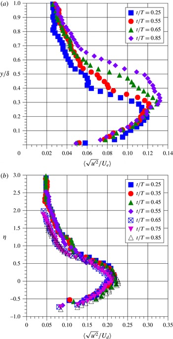
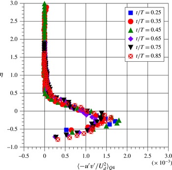
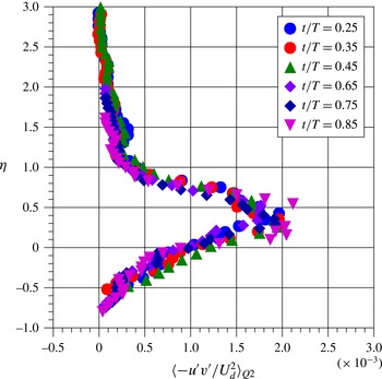
Phase-averaged velocity, turbulence intensity and Q2 and Q4 Reynolds stress profiles at
 $x/L=0.86$
for
 $\unicode[STIX]{x1D6FC}_{q}=3$
and indicated
 $t/T$
value.

Figure 25 presents phase-averaged profiles of the Q2 and Q4 contributions to the Reynolds stress along with the corresponding phase-averaged turbulence intensity and velocity profiles as obtained at
 $x/L=0.86$
on the ramp for several representative times
 $t/T$
during the unsteady cycle. It should be recalled from figure 16 that this
 $x/L$
location exhibits intermittent transitory detachment (
 $\langle \unicode[STIX]{x1D6FE}_{+u}\rangle \approx 0.80$
) during a portion of the plasma-on part of the cycle. In figure 25, the
 $y/\unicode[STIX]{x1D6FF}$
locations of peak turbulence intensity, as indicated by the dashed lines, are shown to coincide with the inflection point of the local phase-averaged velocity profile. Furthermore, at this
 $y/\unicode[STIX]{x1D6FF}$
location, the Q2 and Q4 contributions to the Reynolds stresses have nearly identical values. For time
 $t/T>0.5$
with the plasma on and the severity of the APG increased, the location of the inflection point, the peak turbulence intensity and the
 $y/\unicode[STIX]{x1D6FF}$
location associated with matching contributions of Q2 and Q4 Reynolds stress all shift away from the wall in concert. For every
 $t/T$
value shown, peak Q2 Reynolds stress is located on the high-speed side of the velocity profile inflection point, above the peak turbulence intensity location. In contrast, the peak Reynolds stress due to Q4 sweep events is located on the low-speed side of the inflection point, below the peak turbulence intensity location. In fact, figure 25 shows that the wall-normal variation in the position of contours of peak values of
 $\langle -u^{\prime }v_{Q2}^{\prime }/U_{e}^{2}\rangle$
and
 $\langle -u^{\prime }v_{Q4}^{\prime }/U_{e}^{2}\rangle$
during the unsteady cycle shown previously in figure 24 actually reflects the wall-normal motion of the outer inflection point of the phase-averaged velocity profile. It should be noted that this behaviour was also found to be true for the other
 $x/L$
locations along the ramp.
Schematic showing how coherent spanwise vorticity associated with an inflectional instability in the embedded shear layer gives rise to Q2 and Q4 peak Reynolds stress events.

Taken together, the results shown in figure 25 are consistent with the presence of an embedded shear layer within the APG boundary layer which contains spanwise-oriented coherent vorticity with clockwise rotation that arises from a Kelvin–Helmholtz inflectional instability. This is shown schematically in figure 26. In this view, the coherent vortical structures associated with the embedded shear layer are responsible for the localized peaks in Q4 Reynolds stress on the low-speed side of the shear layer as vortices transfer comparatively high-velocity fluid above the shear layer to the low-speed side
 $(u^{\prime }>0,v^{\prime }<0)$
. Similarly, the Q2 Reynolds stress peak on the high-speed side of the shear layer is the result of comparatively low-speed near-wall fluid being transferred across the shear layer to the high-speed side
 $(u^{\prime }<0,v^{\prime }>0)$
.
The results of the conditional measurements presented in this section suggest that the presence of an embedded shear layer inflectional instability could play a dominant role in the flow physics of the APG turbulent boundary layer. That being the case, consideration is next given to scaling the boundary layer based on embedded shear layer parameters.
5 Embedded shear layer scaling
The Rayleigh inflection point theorem indicates that an inflection point in the base flow velocity profile is a necessary condition for inviscid instability. This, along with experimental results like those shown in figure 25, suggests the potential importance of inflectional instability mechanisms in APG turbulent boundary layers. While it may be argued that the turbulent flow never really ‘sees’ the mean or phase-averaged velocity profile, the existence of an inflection point in the mean is indicative of instantaneous inflectional profiles that would trigger inviscid instability. Further, it has been shown by Wygnanski, Champagne & Marasli (Reference Wygnanski, Champagne and Marasli1986) that inviscid linear stability analysis applied to the mean velocity profile in the far field of a turbulent wake yields eigenmode profiles that exhibit an uncanny resemblance to measured streamwise-component turbulence intensity profiles.
The large spatial growth rates generally associated with inflectional instability will give rise to an embedded shear layer containing coherent large-scale spanwise-oriented vorticity within the unsteady APG boundary layer which will have a large effect on both the spatial and temporal flow development, at least at sufficient distance from the wall. If this is indeed the case, then one may expect embedded shear layer scaling to effectively collapse boundary layer velocity profiles over a significant wall-normal extent.
Figure 27 presents such a proposed embedded shear layer type of scaling for the unsteady APG turbulent boundary layer under consideration here. The relevant length scale is taken to be the local embedded shear layer vorticity thickness,
 $$\begin{eqnarray}\unicode[STIX]{x1D6FF}_{\unicode[STIX]{x1D714}}\left(x,t\right)\equiv \frac{\left(U_{e}-\overline{U}\right)_{IP}}{\left(\text{d}\overline{U}/\text{d}y\right)_{IP}},\end{eqnarray}$$
where the subscript IP denotes that the relevant quantity is to be evaluated at the outermost inflection point of the velocity profile. The relevant velocity scale is taken to be the local velocity defect at the outer inflection point,
 $$\begin{eqnarray}U_{d}\equiv \left(U_{e}-\overline{U}\right)_{IP}.\end{eqnarray}$$
Similarity variables are then defined as
 $$\begin{eqnarray}\unicode[STIX]{x1D702}\equiv \frac{y-y_{IP}}{\unicode[STIX]{x1D6FF}_{\unicode[STIX]{x1D714}}},\quad U^{\ast }\equiv \frac{U_{e}-\overline{U}}{U_{d}}.\end{eqnarray}$$
Figure 28 shows the measured streamwise growth of the embedded shear layer vorticity thickness,
 $\unicode[STIX]{x1D6FF}_{\unicode[STIX]{x1D714}}$
, along the convex ramp section for both the plasma-off and plasma-on end states of the unsteady APG cycle. The vorticity thickness is observed to grow linearly along the ramp section for both cases. The spatial growth rate,
 $\text{d}\unicode[STIX]{x1D6FF}_{\unicode[STIX]{x1D714}}/\text{d}x$
, was obtained from figure 28. With the plasma off, the embedded shear layer grows at a rate of
 $\text{d}\unicode[STIX]{x1D6FF}_{\unicode[STIX]{x1D714}}/\text{d}x=0.078$
, and with the plasma on,
 $\text{d}\unicode[STIX]{x1D6FF}_{\unicode[STIX]{x1D714}}/\text{d}x=0.102$
, an increase of 31 %. These values are well within the range of measured growth rates for planar turbulent shear layers as reported from a number of published experiments (e.g. Oster & Wygnanski Reference Oster and Wygnanski1982). It is also interesting to note that the increase in shear layer growth rate parallels the approximately 30 % increase in local boundary layer thickness between the plasma-on and -off cycle end states.
Illustration of embedded shear layer velocity and length scales (mean velocity profile at
 $x/L=0.86$
, plasma-on case).

Growth of the embedded shear layer vorticity thickness,
 $\unicode[STIX]{x1D6FF}_{\unicode[STIX]{x1D714}}$
, along the ramp for plasma-on and plasma-off end states.

Figure 29 presents phase-averaged APG turbulent boundary layer velocity profiles obtained at
 $x/L=0.86$
at the same representative values of
 $t/T$
shown previously in figure 25 but now presented in terms of embedded shear layer scaling. This figure shows that the time dependence of the phase-averaged velocity profiles has been effectively removed, and the collapse is shown to be remarkable. The scaled profiles are independent of phase,
 $t/T$
, and are very well approximated by a profile of functional form
 $$\begin{eqnarray}U^{\ast }=1-\tanh (\unicode[STIX]{x1D702}).\end{eqnarray}$$
The only significant deviation from the above relation emerges in the near-wall region (i.e. larger values of negative
 $\unicode[STIX]{x1D702}$
), as it must in order to satisfy the no-slip condition as the wall is approached.
Phase-averaged APG turbulent boundary layer profiles at
 $x/L=0.86$
presented in terms of embedded shear layer scaling.

As a basis for comparison with alternate APG turbulent boundary layer scaling, phase-averaged velocity profiles obtained at
 $x/L=0.86$
for a representative range of times in the interval
 $0\leqslant t/T\leqslant 1$
are presented in figure 30(a) in terms of the Zaragola & Smits (Reference Zaragola and Smits1998) velocity defect scaling. This may be compared with the same set of profiles shown in figure 30(b), where embedded shear layer scaling has been employed. It is clear from figure 30 that the embedded shear layer scaling provides a much tighter collapse of the APG turbulent boundary layer profiles.
Comparison of phase-averaged APG turbulent boundary layer profiles at
 $x/L=0.86$
for a range of phase,
 $t/T$
, using (a) the Zaragola–Smits velocity defect scaling and (b) embedded shear layer scaling.

Figure 31 presents time-averaged boundary layer velocity profiles obtained at
 $x/L=0.86$
for both the plasma-on and plasma-off cases in terms of embedded shear layer scaling. This scaling is observed to account for the different APG cases, as both profiles collapse to a common shape that agrees well with (5.4). Figure 32 presents the same time-mean velocity profiles in terms of the Zaragola & Smits (Reference Zaragola and Smits1998) velocity defect scaling, which clearly fails to provide a similar degree of collapse. It is important to also note that the embedded shear layer scaling results presented in figures 29, 30(b) and 31 may be considered as representative of those obtained at other
 $x/L$
locations on the convex ramp.
Comparison of APG turbulent boundary layer mean velocity profiles at
 $x/L=0.86$
for the plasma-on and plasma-off APGs using embedded shear layer scaling.

Comparison of APG turbulent boundary layer mean velocity profiles at
 $x/L=0.86$
for the plasma-on and plasma-off APGs using Zaragola–Smits velocity defect scaling.

Figure 33 presents embedded shear layer scaling applied to mean velocity profiles obtained at several
 $x/L$
locations on the convex ramp surface with the plasma off (attached ramp flow). The resulting collapse indicates that the scaling is also able to account for the spatial variation of the mean velocity for a given non-equilibrium APG environment. Here, the largest deviation appears to be associated with the
 $x/L=0.59$
location, for which the profile has just become inflectional.
Adverse pressure gradient turbulent boundary layer mean velocity profiles at various values of
 $x/L$
for the plasma-off APG using embedded shear layer scaling.

Figure 34(a) presents the phase-averaged streamwise-component turbulence intensity measured at
 $x/L=0.86$
for a representative range of times
 $t/T$
(i.e. phases) in the unsteady pressure gradient cycle. This figure shows both the growth in magnitude of the boundary layer turbulence intensity peak and its movement away from the wall as the APG becomes more severe.
Figure 34(b) presents phase-averaged turbulence intensity profiles at
 $x/L=0.86$
for a wide range of
 $t/T$
values but using the embedded shear layer scaling. The scaling is observed to provide a good collapse of the intensity profiles, particularly for
 $-0.5\leqslant \unicode[STIX]{x1D702}\leqslant 0.75$
. The only deviation is in the outer region of the boundary layer
 $(\unicode[STIX]{x1D702}>1)$
, and this is due primarily to the transient vortex shedding from the airfoil during plasma on/off and off/on parts of the cycle (see figures 7 and 8). Figure 34(b) shows that peak turbulence intensity remains associated with the spatial location of the velocity profile inflection point
 $(\unicode[STIX]{x1D702}=0)$
during the unsteady cycle, and the peak value remains relatively constant with
 $u_{RMS}^{\ast }=\langle \sqrt{u^{\prime 2}}/U_{d}\rangle \approx 0.21$
. Thus,
 $\langle \sqrt{u^{\prime 2}}\rangle$
scales with
 $\langle (U_{e}-U_{d})_{IP}\rangle$
. This scaling is evidence of the prominent role played by the embedded shear layer in the local flow physics of the unsteady APG turbulent boundary layer.
(a) Phase-averaged turbulence intensity profiles for a range of
 $t/T$
during the unsteady cycle as obtained at
 $x/L=0.86$
. (b) The intensity profiles scaled with embedded shear layer parameters.

If large-amplitude Q4 events are a consequence of the embedded shear layer transferring relatively high-momentum fluid from above the shear layer towards the wall, then the induced streamwise velocity fluctuation
 $u^{\prime }\propto U_{e}-\overline{U}_{IP}\equiv U_{d}$
. Hence, the most appropriate scaling for
 $\langle -u^{\prime }v_{Q4}^{\prime }\rangle$
is expected to be
 $\langle U_{d}^{2}\rangle$
. Figure 35 presents
 $\langle -u^{\prime }v^{\prime }/U_{d}^{2}\rangle _{Q4}$
as a function of
 $\unicode[STIX]{x1D702}$
for a representative range of times
 $t/T$
(i.e. phases) during the unsteady cycle. The scaling is observed to provide a remarkable collapse of the Q4 Reynolds stress profiles, with the peak value
 $\left\langle u^{\prime }v^{\prime }/U_{d}^{2}\right\rangle \approx 1.5\times 10^{-3}$
occurring just below the phase-averaged velocity profile inflection point at
 $\unicode[STIX]{x1D702}\approx -0.25$
.
Embedded shear layer scaling of profiles of phase-averaged Q4 Reynolds stress at
 $x/L=0.86$
.

If the Q2 events are associated with the transfer of relatively low-momentum near-wall fluid below the embedded shear layer to the higher-speed side, one would expect that
 $\langle -u^{\prime }v_{Q2}^{\prime }\rangle$
would also scale with the velocity defect,
 $\langle U_{d}\rangle$
. In fact, this is observed to be the case, as is clearly shown in figure 36. This figure presents
 $\langle -u^{\prime }v^{\prime }/U_{d}^{2}\rangle _{Q2}$
as a function of
 $\unicode[STIX]{x1D702}$
for a representative range of times
 $t/T$
(i.e. phases) during the unsteady cycle. The Q2 Reynolds stress profiles exhibit collapse, with a peak Q2 Reynolds stress of
 $\langle -u^{\prime }v^{\prime }/U_{d}^{2}\rangle \approx 1.9\times 10^{-3}$
occurring on the high-speed side of the shear layer at
 $\unicode[STIX]{x1D702}=0.35$
.
Embedded shear layer scaling of profiles of phase-averaged Q2 Reynolds stress at
 $x/L=0.86$
.

Castillo & George (Reference Castillo and George2001) showed that most APG turbulent boundary layer flows are actually in equilibrium in the sense of a constant value of the parameter
 $$\begin{eqnarray}\unicode[STIX]{x1D6EC}\equiv -\frac{\unicode[STIX]{x1D6FF}(x)}{U_{e}(x)}\frac{1}{\text{d}\unicode[STIX]{x1D6FF}/\text{d}x}\frac{\text{d}U_{e}}{\text{d}x}.\end{eqnarray}$$
In their paper, Castillo & George (Reference Castillo and George2001) examined several of the turbulent boundary layer data sets compiled by Coles & Hirst (Reference Coles and Hirst1969) and found that for flows with APG varying from mild to strong, the values of
 $\unicode[STIX]{x1D6EC}$
varied surprisingly little,
 $0.189\leqslant \unicode[STIX]{x1D6EC}\leqslant 0.279$
. Given the self-similarity in both time and space achieved by application of embedded shear layer scaling, it is of interest to examine the values of the
 $\unicode[STIX]{x1D6EC}$
parameter for the convex ramp flow for the plasma-on, plasma-off and time mean of the unsteady flow cases. The results show that the plasma-off case exhibits values near
 $\unicode[STIX]{x1D6EC}\approx 0.23$
for
 $x/L<0.6$
, but the
 $\unicode[STIX]{x1D6EC}$
value subsequently exhibits significant streamwise variation farther downstream, leading to reduced values approaching
 $\unicode[STIX]{x1D6EC}\approx 0.1$
. The values for the plasma-on case are initially lower. For example,
 $\unicode[STIX]{x1D6EC}\approx 0.17$
at
 $x/L=0.62$
. This value is further reduced with increased streamwise distance. Not surprisingly, results based on the time mean of the unsteady case exhibit values of
 $\unicode[STIX]{x1D6EC}$
between the plasma-on and -off cases. These results show that for the APG turbulent boundary layer on the convex ramp surface, the flow is clearly in a non-equilibrium state in terms of the streamwise variation of the Castillo and George parameter,
 $\unicode[STIX]{x1D6EC}$
, and this makes the self-similarity exhibited by the embedded shear layer scaling all the more remarkable.
Wall-normal variation in
 $\overline{T}_{Q2}^{\ast }$
and
 $\overline{T}_{Q4}^{\ast }$
at
 $x/L=0.93$
for the plasma-off pressure gradient. It should be noted that
 $\overline{T}_{Q2}^{\ast }=\overline{T}_{Q4}^{\ast }=7.2$
at the outermost inflection point of the mean velocity profile.

6 Discussion
6.1 Additional evidence for embedded shear layer instability
Further evidence for the existence of an embedded shear layer in the APG turbulent boundary layer associated with the outer inflection point can be found in reconsidering the previously presented mean time between strong Q2 and Q4 Reynolds-stress-producing events. As an example, figure 37 presents both
 $\overline{T}_{Q2}^{\ast }\equiv \overline{T}_{Q2}\,U_{e}/\unicode[STIX]{x1D6FF}$
and
 $\overline{T}_{Q4}^{\ast }\equiv \overline{T}_{Q4}\,U_{e}/\unicode[STIX]{x1D6FF}$
versus
 $y/\unicode[STIX]{x1D6FF}$
as obtained at
 $x/L\quad =$
0.93 for the plasma-off case. Reference to figure 16 indicates that the boundary layer remains fully attached at this location. The hyperbolic hole size was
 $\unicode[STIX]{x1D6FC}_{q}=4$
, so that these conditional measurements capture the strongest ejection and sweep events. It is interesting to note that at the wall-normal location of the outer inflection point (denoted by an arrow in figure 37),
 $\overline{T}_{Q2}^{\ast }=\overline{T}_{Q4}^{\ast }=7.2$
. That is, the local mean period between strong ejection and sweep events is identical at the outer inflection point of the mean velocity profile. In terms of the local mean frequency of these events, we have
 $\overline{T}\unicode[STIX]{x1D6FF}/U_{e}=7.2$
, so that
 $\unicode[STIX]{x1D6FF}/\overline{T}U_{e}=f\unicode[STIX]{x1D6FF}/U_{e}=0.139$
. This may be rescaled to a form more typical of that used in free shear layer instability as follows:
 $$\begin{eqnarray}\frac{f\unicode[STIX]{x1D703}}{U_{e}}=\frac{f\unicode[STIX]{x1D6FF}}{U_{e}}\frac{\unicode[STIX]{x1D6FF}_{\unicode[STIX]{x1D714}}}{\unicode[STIX]{x1D6FF}}\frac{\unicode[STIX]{x1D703}}{\unicode[STIX]{x1D6FF}_{\unicode[STIX]{x1D714}}}.\end{eqnarray}$$
From the local measured mean velocity profile,
 $\unicode[STIX]{x1D6FF}_{\unicode[STIX]{x1D714}}/\unicode[STIX]{x1D6FF}=0.22$
and
 $\unicode[STIX]{x1D703}/\unicode[STIX]{x1D6FF}_{\unicode[STIX]{x1D714}}=0.39$
. Using these values, one finds that the scaled frequency between both strong burst and sweep events is given by
 $$\begin{eqnarray}\frac{f\unicode[STIX]{x1D703}}{U_{e}}=0.012.\end{eqnarray}$$
This value of the scaled frequency between strong Q2 and Q4 events is also representative of those obtained at other
 $x/L$
locations on the convex ramp, and, more importantly, is well within the range of most unstable free shear layer instability frequencies reported in the literature (e.g. Thomas Reference Thomas1991). In particular, published values for the most unstable free shear layer instability frequency fall within the range
 $0.009\leqslant f\unicode[STIX]{x1D703}/U_{e}\leqslant 0.015$
, with most of the variation accounted for by facility-dependent spatially coherent forcing (Gutmark & Ho Reference Gutmark and Ho1983). It is important to note that this range of frequencies is two orders of magnitude higher than the time scale associated with the imposed
 $\text{d}U_{e}/\text{d}t$
due to plasma flow control. That this instability frequency matches those of both strong Q2 and Q4 Reynolds stress-producing events occurring near the outer inflection point in the APG turbulent boundary layer strongly suggests that they are a manifestation of coherent spanwise vorticity residing in the embedded shear layer.
6.2 The role of the upper and lower APG turbulent boundary layer inflection points
For a sufficiently large APG, the turbulent boundary layer mean velocity profile will develop two inflection points, as shown schematically in figure 38. The experimental results presented in this investigation indicate that the local flow physics is, in large part, dominated by an embedded shear layer inflectional instability that is associated with the outer inflection point. The inner inflection point seems not to play a similar role. In order to investigate why this is the case, consideration is given to the Rayleigh–Fjørtoft theorem, which formally states that a necessary condition for inviscid instability is that
 $U^{\prime \prime }(U-U_{IP})<0$
somewhere in the flow field. Here, primes denote differentiation with respect to the wall-normal coordinate. In practice, the Rayleigh–Fjørtoft theorem is viewed as both a necessary and a sufficient condition for inviscid instability. Although counter-examples of sufficiency conditions can be found, they are rare (see Drazin Reference Drazin2002). As shown in figure 38(a), just below the upper inflection point,
 $(U-U_{IP})<0$
while
 $U^{\prime \prime }>0$
, so that
 $U^{\prime \prime }(U-U_{IP})<0$
. Just above the upper inflection point,
 $(U-U_{IP})>0$
while
 $U^{\prime \prime }<0$
, such that again
 $U^{\prime \prime }(U-U_{IP})<0$
. Thus, the upper inflection point of the APG turbulent boundary layer velocity profile satisfies the necessary and sufficient condition for inviscid instability.
Application of the Rayleigh–Fjørtoft theorem to the APG turbulent boundary layer mean velocity profile, confirming the inviscid instability of the outer inflection point.

In contrast, for the lower APG turbulent boundary layer inflection point, a similar analysis presented in figure 38(b) shows that
 $U^{\prime \prime }(U-U_{IP})>0$
both above and below the lower inflection point, thereby failing the Rayleigh–Fjørtoft requirement for inviscid instability. Hence, the Rayleigh–Fjørtoft theorem indicates that only the outer APG turbulent boundary layer profile inflection point is associated with inviscid instability. This is fully consistent with the results of this experimental investigation and the associated scaling, which clearly shows the influence of the embedded shear layer associated with the outer inflection point.
At this point, it should be noted that the inviscid inflectional instability mechanism described here is quite distinct from, but certainly does not preclude, the viscous linear instability of low-speed streaks in APG wall-bounded turbulent flow. For example, in direct numerical simulations by Marquillie, Ehrenstein & Laval (Reference Marquillie, Ehrenstein and Laval2011), the viscous linear stability of low-speed streaks in APG turbulent channel flow was examined. Near-wall streaks in cross-flow planes and averaged in time were superimposed on the mean streamwise velocity profile, and this formed the base flow for stability analysis. Spanwise symmetric instability modes were observed for APG flow with wall-normal inflection points. This instability appears to be correlated with near-wall peaks in turbulent kinetic energy.
6.3 Regarding the generic applicability of embedded shear layer scaling
A natural question arises as to whether the embedded shear layer instability plays as prominent a role in the flow physics of all APG turbulent boundary layers (with inflectional mean velocity profiles) as was the case for the unsteady boundary layer documented in this paper. A related question is whether the embedded shear layer scaling is generically applicable to APG turbulent boundary layers with spatially varying APGs. As a first step at addressing this question, consideration is given to one of the APG turbulent boundary layer flows investigated by Marusic & Perry (Reference Marusic and Perry1995). In particular, consideration is given to their experiment involving a flat-plate ZPG turbulent boundary layer that subsequently experiences an imposed constant APG. The flow in question was designated by Marusic and Perry as Flow 10APG. Their data set includes both measured mean velocity and Reynolds stress profiles obtained at six streamwise locations within the region of imposed APG. For the last three locations, the Coles wake parameter,
 $\unicode[STIX]{x1D6F1}$
, is sufficiently large that the mean velocity profiles have become inflectional. These locations along with their corresponding values of the Coles wake parameter,
 $\unicode[STIX]{x1D6F1}$
, the Clauser parameter,
 $\unicode[STIX]{x1D6FD}$
, and
 $Re_{\unicode[STIX]{x1D703}}$
are listed in table 2.
Flow 10APG parameters (Marusic & Perry Reference Marusic and Perry1995).

Figure 39 compares the measured mean velocity profiles in terms of conventional outer variable scaling (figure 39
a) with the same embedded shear layer profile scaling as used in the current investigation (figure 39
b). As was the case in the current study, figure 39(b) shows that the embedded shear layer scaling provides a very tight collapse of the mean velocity profiles over a significant wall-normal extent. Furthermore, the only significant deviation from self-similar behaviour occurs at the largest negative values of
 $\unicode[STIX]{x1D702}$
, which correspond to near-wall locations below the embedded shear layer in order to satisfy the no-slip condition as the wall is approached. The degree of deviation from self-similarity appears to decrease as the Coles wake parameter
 $\unicode[STIX]{x1D6F1}$
(and
 $Re_{\unicode[STIX]{x1D703}}$
) increases.
Adverse pressure gradient turbulent boundary layer Flow10APG (Marusic & Perry Reference Marusic and Perry1995) mean velocity profiles in (a) outer variable scaling and (b) embedded shear layer scaling.

Figure 40 presents profiles of both streamwise-component turbulence intensity and Reynolds shear stress for Flow 10APG in terms of conventional outer variable scaling. The profiles are shown at the same streamwise locations as for the mean flow profiles shown in figure 39. Figure 41 presents the same turbulence intensity and Reynolds stress profiles expressed in terms of embedded shear layer scaling. The ability of the scaling to fully collapse both the turbulence intensity and the Reynolds stress profiles is apparent. In addition, the peak turbulence intensity is
 $\sqrt{\overline{{u^{\prime }\,}^{2}}}/U_{d}=0.21$
and occurs at
 $\unicode[STIX]{x1D702}=0$
, which is identical to the results obtained from application of embedded shear layer scaling to the phase-averaged turbulence intensity measurements obtained in the unsteady APG turbulent boundary layer that is the focus of the current study (see figure 34
b).
(a) Streamwise-component turbulence intensity and (b) Reynolds stress from Flow 10APG (Marusic & Perry Reference Marusic and Perry1995) in terms of conventional outer variable scaling.

(a) Streamwise-component turbulence intensity and (b) Reynolds stress from Flow 10APG (Marusic & Perry Reference Marusic and Perry1995) in terms of embedded shear layer scaling.

Adverse pressure gradient turbulent boundary layer flows from Coles & Hirst (Reference Coles and Hirst1969).

In order to further assess the generic applicability of embedded shear layer scaling, consideration is also given to several of the APG turbulent boundary layer data sets from the AFOSR-IFP-Stanford Conference compiled by Coles & Hirst (Reference Coles and Hirst1969). In particular, embedded shear layer scaling was applied to the wide variety of APG turbulent boundary layer flows listed in table 3.
The result of applying the embedded shear layer scaling to each flow is shown in figure 42. For each scaled profile, the wake parameter,
 $\unicode[STIX]{x1D6F1}$
, is indicated along with the momentum thickness Reynolds number,
 $Re_{\unicode[STIX]{x1D703}}$
. Irrespective of the flow-field geometry, embedded shear layer scaling is observed to provide a very tight collapse of the boundary layer mean velocity profiles in each experiment. Of particular interest is flow 2900 shown in figure 42(c). It should be noted that these data extend to
 $Re_{\unicode[STIX]{x1D703}}=100\,000$
, showing that the scaling holds over a very large Reynolds number range. It should be noted also that, in each case, deviation from self-similar behaviour only occurs close to the wall (i.e. the largest negative values of
 $\unicode[STIX]{x1D702}$
), as it must in order to satisfy the no-slip condition. However, the near-wall deviation from self-similar behaviour clearly depends on the wake parameter,
 $\unicode[STIX]{x1D6F1}$
. In particular, as the
 $\unicode[STIX]{x1D6F1}$
parameter increases, the deviation from self-similar behaviour moves closer to the wall. In other words, larger values of the
 $\unicode[STIX]{x1D6F1}$
parameter are associated with a greater wall-normal extent of self-similar behaviour and associated influence of the embedded shear layer instability mechanism. Figure 42(e) presents scaled mean velocity profiles for flow 2300, which involves an APG turbulent boundary layer with approximately constant
 $\unicode[STIX]{x1D6F1}$
parameter. Consequently, all profiles are shown to deviate from self-similarity at the same wall-normal location. Finally, figure 42(f) compares all of the scaled profiles and demonstrates that they all nicely collapse to a common profile shape with the extent of self-similar behaviour a function of
 $\unicode[STIX]{x1D6F1}$
.
Embedded shear layer scaling of APG turbulent boundary layer profiles from the experimental data sets compiled by Coles & Hirst (Reference Coles and Hirst1969). In each case, the
 $\unicode[STIX]{x1D6F1}$
parameter and
 $Re_{\unicode[STIX]{x1D703}}$
value are indicated. (a) Flow 1200: Ludwieg & Tillmann; (b) Flow 2100: Schubauer & Klebanoff; (c) Flow 2900: Perry; (d) Flow 3500: Newman; (e) Flow 2300: Clauser, flow 2; (f) All data.

6.4 Concluding remarks
The results of this investigation clearly indicate that for a turbulent boundary layer exposed to an APG of sufficient magnitude to give rise to inflectional mean or phase-averaged velocity profiles, the flow physics is, in large part, dominated by the existence of an embedded shear layer associated with the inviscid instability of the outer inflection point. This is found to be true for fully attached APG boundary layer flow; separation is certainly not a prerequisite for the existence of the embedded shear layer. It is shown that the boundary layer turbulence intensity peak corresponds to the instantaneous wall-normal location of the outer velocity profile inflection point. Similarly, the location of the peak ejection event (Q2) contribution to Reynolds stress is shown to occur on the high-velocity side of the embedded shear layer while the peak sweep event (Q4) contribution peaks on the low-velocity side. This result is consistent with the existence of clockwise spanwise-oriented coherent vorticity within the embedded shear layer. Further evidence for this comes from the fact that the mean frequency of large-amplitude burst and sweep events near the inflection point when scaled on embedded shear layer parameters corresponds to a Strouhal number consistent with the most unstable shear layer instability frequency. Application of the Rayleigh–Fjørtoft theorem shows that the outer inflection point is inviscidly unstable while the inner is not – a result fully consistent with the experimental results.
Using embedded shear layer scaling parameters in the form of the shear layer vorticity thickness and velocity defect at the upper inflection point, both mean and phase-averaged boundary layer velocity profiles exhibit similarity in both space and time over a large wall-normal extent, with the only deviation occurring in the near-wall region, as it must in order to satisfy the no-slip condition. The scaled velocity profile is well approximated by
 $U^{\ast }=1-\tanh (\unicode[STIX]{x1D702})$
. In a similar manner, profiles of streamwise-component turbulence intensity and Reynolds stress also exhibit similarity when scaled with embedded shear layer parameters.
The application of the embedded shear layer scaling to the APG turbulent boundary layer measurements of Marusic & Perry (Reference Marusic and Perry1995) and several of the APG turbulent boundary layer data sets from the AFOSR-IFP-Stanford Conference compiled by Coles & Hirst (Reference Coles and Hirst1969) clearly demonstrates the generic applicability of this scaling over a wide range of flow-field geometries and to very large Reynolds numbers.
Finally, we conjecture that the embedded shear layer may well be a generic feature of all APG turbulent boundary layers irrespective of whether or not the mean velocity profile is inflectional. Although more apparent in APG boundary layers with inflectional mean velocity profiles, transient and non-localized inflectional instability could well account for the enhancement of outer large-scale structure documented in previous studies (e.g. Harun et al. Reference Harun, Monty, Mathis and Marusic2013) of APG turbulent boundary layers.
Acknowledgements
The authors would like to recognize the support of the US Army Research Office under grant W911NF-07-1-0122 monitored by T. Doligalski.