2. Theoretical framework

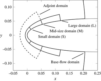
The stability of the steady flow around the front part of a symmetric Joukowski profile, as sketched in figure 1, is investigated. For simplification, the incompressible spanwise-invariant time-dependent Navier–Stokes equations are described in compact form by $\mathscr{R}(\partial _{t},\partial _{x},\partial _{y},k_{z};\boldsymbol{Q})$ where $k_{z}$ is the spanwise wavenumber and $\boldsymbol{Q}=\{U,V,W,P\}$ ; the linearized analogue with additional forcing $\boldsymbol{f}$ is given by the operator $\mathscr{L}(\partial _{t},\partial _{x},\partial _{y},k_{z},\bar{\boldsymbol{Q}})$ defined by

where $\bar{\boldsymbol{Q}}=\{\bar{U},\bar{V},\bar{W},\bar{P}\}$ denotes the steady spanwise-invariant ( $k_{z}=0$ ) base-state velocity components and pressure, and $\boldsymbol{q}=\{u,v,w,p\}$ their perturbation counterparts. An explicit forcing $\boldsymbol{f}$ is assumed.

Figure 1.

Outline of the computational domains: the largest domain, extending beyond the axes range, is used for the base-flow computations. Three domains, characterized by the same extent in the direction normal to the profile but with different downstream extents, are used for the computations of the eigenvalues and eigenvectors. An additional domain (dashed) is used for the computation of the adjoint modes. The grid spacing is kept unchanged in all computations, while the number of grid points adapts according to the changes in the domain size.

Our main objectives are to describe (i) the dynamics of small perturbations $\boldsymbol{q}$ to a given steady base flow $\bar{\boldsymbol{Q}}$ and (ii) the receptivity of these perturbations to external forcing and their sensitivity to structural changes in the governing equations (2.1), e.g. changes in the base flow $\bar{\boldsymbol{Q}}$ . Receptivity and sensitivity are the fundamental concepts that need to be considered for any passive and active manipulation of the flow.

It is convenient to describe the perturbations in Fourier space rather than in physical space. Let $\hat{\cdot }$ denote temporally Fourier-transformed quantities. For a full description of the theoretical framework the reader is referred to the work of Giannetti & Luchini (Reference Giannetti and Luchini2003, Reference Giannetti and Luchini2007) and Marquet, Sipp & Jacquin (Reference Marquet, Sipp and Jacquin2008). Even though we can formulate a receptivity and sensitivity analysis based on a wide range of output measures, we choose the induced response amplitude $\hat{A}$ in the least stable mode for receptivity studies, and the least stable eigenvalue ${\it\sigma}$ for sensitivity studies. In this context, receptivity can be interpreted as the variation ${\it\delta}\hat{A}$ of the response amplitude $\hat{A}$ associated with a variation ${\it\delta}\hat{\boldsymbol{f}}$ in the forcing $\hat{\boldsymbol{f}}$ . Sensitivity can be interpreted as the variation ${\it\delta}{\it\sigma}$ of the eigenvalue ${\it\sigma}$ associated with a change ${\it\delta}\hat{\mathscr{L}}$ in the structure of the governing equations  $\hat{\mathscr{L}}$ .

According to the abovementioned studies receptivity is mathematically defined as

where $\hat{{\bf\lambda}}$ is the adjoint eigenvector, i.e. the eigenvector of $\hat{\mathscr{L}}^{+}$ (the adjoint of $\hat{\mathscr{L}}$ ) obtained after defining a suitable inner product $\langle \cdot ,\cdot \rangle$ , e.g.  $\langle a,b\rangle =\int \!a^{H}b\;\text{d}{\it\Omega}$ . The adjoint eigenvector arises in this formulation from the fact that, in a variational formulation of the receptivity or sensitivity problem, the governing equations (2.1) are enforced by Lagrange multipliers or adjoint variables. In a similar way, sensitivity is defined as

where $\hat{\boldsymbol{q}}$ is the direct eigenvector corresponding to $\hat{{\bf\lambda}}$ .

The adjoint eigenfunction is used in the definition of receptivity (2.2) and sensitivity (2.3) to identify the most receptive and sensitive regions in the physical domain: according to the above definitions, a spatially localized perturbation ${\it\delta}\hat{\boldsymbol{f}}$ of the forcing is more effective in changing the response amplitude where the adjoint field is the largest; a localized perturbation ${\it\delta}\hat{\mathscr{L}}$ of the linear operator $\hat{\mathscr{L}}$ is most effective where the pointwise product of the direct and adjoint fields is the largest. Giannetti & Luchini (Reference Giannetti and Luchini2007) name this latter region the wavemaker: if one interprets the term ${\it\delta}\hat{\mathscr{L}}\hat{\boldsymbol{q}}$ as a localized feedback forcing due to the perturbations in the operator, this is the region where the strongest perturbations $\hat{\boldsymbol{q}}$ and the highest receptivity $\hat{{\bf\lambda}}$ line up and most efficiently modify the flow field structure.

In short, we see that receptivity describes the response to additive changes to the governing equations, modelling external sources of influence (such as free-stream turbulence or wall roughness), while sensitivity describes the response to structural changes in the governing equations, modelling internal sources of influence (such as base-flow modifications or changes in geometry). In either case, the adjoint variable is instrumental in identifying receptive and sensitive regions of the flow.

3. Global modes, sensitivity and receptivity of the swept leading-edge region

In this section, the results of the global stability, sensitivity and receptivity analyses are presented for the case of a swept-wing boundary layer in a domain extending beyond the region of validity of the swept Hiemenz flow. These results are interpreted in light of what has been discussed in the previous section. Attention is focused on identifying the most receptive and sensitive regions governing the perturbation dynamics in terms of changes in the response amplitude and complex eigenvalues respectively.

A symmetric Joukowski profile with a dimensionless leading-edge radius $r/C=0.016$ , where $C$ denotes the chord length, is considered. The extents of the computational domains used in our analysis are presented in figure 1: eigenvalues and eigenvectors are computed in three domains of different chordwise extent (small, medium and large), while a fourth domain (dashed) is used in the computation of the adjoint eigenfunctions. The mesh spacing, as shown in the grey inset of figure 3(d), is kept unchanged for all domains: larger domains are meshed using a larger number of mesh points.

The various Reynolds numbers commonly used in attachment-line boundary layer analyses are

where $U_{\infty }$ and $W_{\infty }$ are the chordwise and spanwise free-stream velocity components, $r$ is the leading-edge radius, ${\it\delta}=\sqrt{{\it\nu}/S}$ is the viscous length scale, ${\it\nu}$ is the kinematic viscosity and $S=U_{\infty }/r$ is the strain rate at the attachment line for the inviscid flow around a cylinder with radius equal to the leading-edge radius. Computations are performed for a chord-based Reynolds number $\mathit{Re}_{C}=10^{6}$ and a sweep angle ${\it\Lambda}=45^{\circ }$ , corresponding to an attachment-line radius-based Reynolds number $\mathit{Re}_{r}=16\,000$ and a sweep Reynolds number $\mathit{Re}_{s}=\sqrt{\mathit{Re }_{r}}\tan {\it\Lambda}=126$ .

For such parameter settings Lin & Malik (Reference Lin and Malik1996, Reference Lin and Malik1997) and Obrist & Schmid (Reference Obrist and Schmid2003a ) determined that the local steady swept Hiemenz flow is linearly stable and that instabilities arise beyond a critical sweep Reynolds number $\mathit{Re}_{s}$ of approximately 600. Similarly, in the global stability analysis of Mack & Schmid (Reference Mack and Schmid2011b ) for the supersonic flow regime a critical sweep Reynolds number $\mathit{Re}_{s}$ of approximately 600 has been determined.

Maintaining the current sweep angle and leading-edge radius, a sweep Reynolds number $\mathit{Re}_{s}$ of 600 would correspond to a chord-based Reynolds number of $\mathit{Re}_{C}=\mathit{Re}_{s}^{2}\,C/r=22.5\times 10^{6}$ , which is beyond our numerical capabilities for the time being. In spite of the fact that the Reynolds number under consideration is subcritical, it is expected that the shape of the spectrum and the spatial structure of the eigenfunctions will not change appreciably as the Reynolds number is changed from subcritical to supercritical. As subsequently shown, comparison between the present results and the literature corroborates this line of thought. It should also be remarked that transition induced by cross-flow vortices is known to occur at much lower Reynolds numbers than the critical one based on linear analysis: for example, the experimental results of Dagenhart & Saric (Reference Dagenhart and Saric1999) identify cross-flow vortices for chord-based Reynolds numbers as low as $\mathit{Re}_{C}\approx 2\times 10^{6}$ .

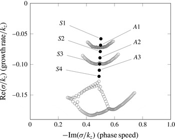
Let ${\it\lambda}_{z}$ and ${\it\delta}_{99}$ denote the spanwise wavelength and the spanwise boundary layer thickness at the attachment line respectively. The spectrum of the linearized Navier–Stokes operator (2.1) for a spanwise wavenumber $k_{z}=4000$ – corresponding to ${\it\lambda}_{z}/{\it\delta}_{99}\simeq 4$ – is computed for the three domains S, M and L of figure 1. A second-order finite-difference scheme is employed for the numerical discretization of the linearized operator on a conformally mapped boundary-fitted grid. The spectrum is indicated with solid black symbols in figure 2. It is composed of a single branch of eigenvalues characterized by a nearly constant phase speed of $c_{r}=0.5$ . Inspection of the eigenvectors reveals that modes with spatially symmetric ( $S1,S2,\dots$ ) and antisymmetric ( $A1,A2,\dots$ ) structure with respect to the attachment line alternate while moving from the least stable eigenvalue to more stable ones. This result is consistent with the local findings of Lin & Malik (Reference Lin and Malik1996, Reference Lin and Malik1997): in the unstable parameter range these authors identified a single branch of constant phase speed $c_{r}=0.35$ consisting of alternating symmetric and antisymmetric modes.

Figure 2.

Eigenvalues for $\mathit{Re}_{C}=10^{6},k_{z}=4000~({\it\lambda}_{z}/{\it\delta}_{99}\simeq 4)$ . The computed spectrum consists of a single branch – solid black symbols – of modes travelling at roughly the same phase speed $-\text{Im}({\it\sigma}/k_{z})\approx 0.5$ in the spanwise direction. The corresponding eigenvectors present spatial structures that are alternatingly symmetric ( $S1,S2,\dots$ ) and antisymmetric ( $A1,A2,\dots$ ) with respect to the attachment line when moving from the least stable to the most stable mode. The eigenvalues have been computed for three different domain sizes. For the large domain, only $S1$ and $A1$ are recovered. For the mid-sized domain, $S1,A1,S2$ and $A2$ are captured, and for the small domain all seven black eigenvalues are obtained. The grey open circles represent eigenvalues belonging to the pseudo-spectrum.

The computation for the large domain (L) yields only the $S1$ and $A1$ eigenvalues, together with the pseudo-spectrum represented by the curved branch in grey open circles right below $A1$ . The mid-sized domain (M) yields all four eigenvalues from $S1$ to $A2$ , and its pseudo-spectrum is represented by the curved branch in grey open circles below $A2$ . Finally, the smallest domain returns all seven eigenvalues $S1$ to $S4$ , and its pseudo-spectrum lies below $S4$ . 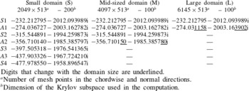For comparison, the eigenvalues computed in the three domains are reported in table 1 with six decimal digits. The digits differing from the values obtained for the small domain are underlined. It can be seen that the least stable eigenvalue $S1$ is the same in all three domains. The $A1$ mode has the same value for the small-sized and mid-sized domains, but the value obtained for the larger domain differs in the last four significant digits. The same is repeated for the $S2$ and $A2$ modes when comparing the small-sized and the mid-sized domains: the $S2$ eigenvalue matches well while $A2$ differs in the last two significant digits. Counterintuitively, computations on larger domains return fewer eigenvalues for numerical reasons. A Krylov–Schur iterative method is employed for the eigenvalue computation in this work. Because of memory limitations, the increase in the number of degrees of freedom – required to maintain a constant mesh spacing – is not matched by an increase in the dimensionality of the Krylov subspace: 100 vectors have been used for both the mid-sized and large domains despite the fact that the number of degrees of freedom increases by a factor of 1.5. For the small domain, 200 vectors have been used. For numerical reasons, the more precise results are obtained for the small domain where only a minor part of the flow structure is resolved. Full details on the numerical approach are reported in Meneghello (Reference Meneghello2013).

Table 1.

Computed eigenvalues.

Digits that change with the domain size are underlined.

a Number of mesh points in the chordwise and normal directions.

b Dimension of the Krylov subspace used in the computation.

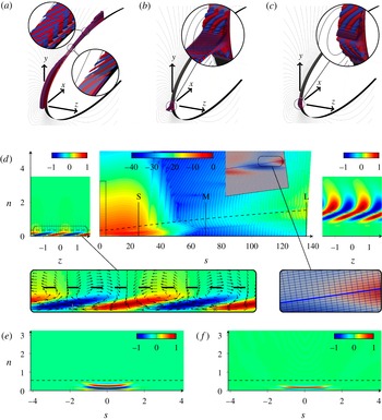
The spectrum and the eigenvectors are now analysed in terms of local stability considerations in an attempt to understand why the location of the eigenvalues in the complex plane is not affected by the position of the outflow boundary. To this end, figure 3 displays the direct and adjoint eigenvectors as well as the wavemaker for the least stable $S1$ eigenvalue by both isocontours of the real part of the chordwise $u$ velocity component of the eigenvectors (figure 3 a–c) and its cross-cuts in a frame of reference defined by a curvilinear chordwise coordinate $s$ , a wall normal coordinate $n$ and a spanwise coordinate $z$ , expressed in thousandths of chord length.

Figure 3(a,d) represent the direct eigenvector covering the full computational domain and growing exponentially towards the outflow boundary of the largest domain. The outflow boundary for each domain is marked by vertical lines and the letters S, M and L. Three regions displaying distinct spatial structures may be identified along the chordwise $s$ coordinate.

Figure 3.

Real part of the chordwise $\hat{u}$ component of the (a,d) direct and (b,e) adjoint eigenvectors and (c, f) wavemaker associated with the least stable $S1$ mode. Red and blue in (a–c) denote positive and negative isocountours respectively; cross-sections are shown in colour in (d–f). In the centre panel of (d), the chordwise $s$ -direction is compressed and a logarithmic colour scale is used. S, M and L denote the outflow boundaries for the three domains. The rectangle at the origin delimits half the domain shown in (e–f). The grey inset shows the numerical grid in a domain close to the outflow boundary with identically scaled horizontal and vertical axes. The left and right panels of (d) display spanwise-normal $s{-}n$ sections close to the attachment line and in the crossflow region, respectively (colour in linear scale). The direct eigenvector extends across the entire computational domain and shows features characteristic of both attachment-line modes and crossflow modes, as obtained by local analysis. The adjoint eigenvector and the wavemaker are localised in a very small region extending only a few boundary layer thicknesses across the attachment line. The spanwise ${\it\delta}_{99}$ boundary layer thickness is indicated by dashed lines. Coordinates are in thousandths of the chord length  $C$ .

1. (i) Close to the attachment line, the eigenvector has a spatial shape corresponding to the local attachment-line modes of swept Hiemenz flow as described in Lin & Malik (Reference Lin and Malik1996). Counter-rotating vortices aligned in the chordwise direction lift low-momentum flow from the wall and push high-momentum flow towards the wall, generating alternating low- and high-chordwise-velocity streaks visible in the $z$ – $n$ section on the left of figure 3(d). Lin & Malik (Reference Lin and Malik1996) and Mack et al. (Reference Mack, Schmid and Sesterhenn2008) identified similar features in their respectively local and global analyses of swept Hiemenz flow and compressible leading-edge flow.

2. (ii) A transition region downstream of the attachment-line region shows a decrease in the eigenvector of nearly 10 orders of magnitude, as can be seen in the cross-cut presented in the central panel of figure 3(d) as well as in the magnified inset of figure 3(a). After the decay of attachment-line features, cross-flow-vortex features start to form just below the ${\it\delta}_{99}$ boundary layer thickness.

3. (iii) Downstream of the transition region, cross-flow vortices, aligned with the base flow at an angle of 45° with respect to the chord, increase exponentially in magnitude. In addition, streamwise-velocity streaks are no longer attached to the wall; instead, they develop across the ${\it\delta}_{99}$ boundary layer thickness.

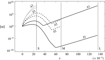
As first presented in Mack et al. (Reference Mack, Schmid and Sesterhenn2008), it is remarkable to note the coexistence, in the same eigenvector, of attachment-line features and cross-flow features, both of which were previously identified in separate local analyses of distinct regions in the boundary layer. Figure 4 displays the magnitude of the first six eigenvectors as a function of the chordwise distance $s$ : the continuous connection between the local attachment line and the local cross-flow-vortex instability, the exponential decay of the attachment-line structure in the chordwise direction by 10 orders of magnitude and the subsequent exponential growth of the cross-flow-vortex structures is made even clearer. Vertical lines mark the outflow boundary for the different domains. It has to be recalled that the $S1$ and $A1$ modes are obtained in all domains, not only in the largest one. The large spatial growth of the eigenfunctions displayed in figure 4 may suggest the dominance of the A1 mode in the cross-flow region; it should, however, be noted that the eigenfunctions have been normalized to attain unit energy density in the attachment line. For a valid assessment of the relative prominence of the (least stable) $S1$ or the $A1$ mode one has to account for their temporal decay rates as well as their respective susceptibility to external noise sources.

Figure 4.

Magnitude of the first six eigenvectors as a function of the chordwise distance $s$ . The eigenvectors have been normalized to unit energy density in the attachment line. Vertical lines mark the outflow boundaries for the S, M and L domains. All eigenvectors exhibit an initial algebraic growth in space, followed by an exponential decay of the attachment-line structure, eventually giving way to an exponential growth of the cross-flow-like structure. A connection between the two local stability structures is evident.

The adjoint eigenvector shows a completely different picture: it is concentrated very close to the attachment line. According to figure 3(e) the adjoint eigenvector is negligible outside a very small region extending a few boundary layer thicknesses across the attachment line in the chordwise $s$ direction. According to our definition of receptivity given by (2.2), this is the most effective region to apply a control forcing in order to modify the response amplitude $\hat{A}$ . In other words, this same region is most effective in promoting the exponential growth of cross-flow-like structures further downstream. It should also be noted that undesirable forcing due to free-stream turbulence would be most disruptive in this high-receptivity region.

In a similar manner the wavemaker – defined by (2.3) – covers a region localized within a single boundary layer thickness which is even smaller than the region covered by the adjoint mode: structural modifications ${\it\delta}\hat{\mathscr{L}}$ of the operator $\hat{\mathscr{L}}$ outside this region have only negligible influence on the location of the eigenvalue $S1$ . This is true also for the structural modifications associated with the location of the outflow boundary – or of the actual numerical implementation of the outflow boundary condition, as shown by table 1.

The localization of the wavemaker in a surprisingly small region close to the attachment line also implies that the local stability results obtained for swept Hiemenz flow by Hall et al. (Reference Hall, Malik and Poll1984) and Lin & Malik (Reference Lin and Malik1996), possibly including curvature corrections as in Lin & Malik (Reference Lin and Malik1997), still hold for the entire leading-edge region. The relevance of previous local stability analyses has therefore been established: the computed spectrum does not change as long as the region covered by the adjoint eigenvector and the wavemaker is correctly represented. As can be seen from figures 3(d) and 4, in the smaller computational domain, extending only $2.5\,\%$ of chord downstream of the attachment line, none of the cross-flow instabilities are accounted for and even the attachment-line instability is truncated close to the location of maximum magnitude. The global eigenvalue is nonetheless correctly calculated.

Our spectral and adjoint analysis uncovered only travelling global structures with support in the attachment line and the boundary layer downstream, and despite a careful and methodical search, no stationary modes have been found. Recalling the existence of two families of cross-flow modes (as discussed, e.g. in Dagenhart & Saric (Reference Dagenhart and Saric1999)), our study can only draw conclusions about the receptivity to travelling modes, in which case we find a high and very localized receptivity in the vicinity of the attachment line. The relative dominance of these two receptivity processes – roughness induced via stationary modes or environmentally induced via travelling modes – depends on the specific flow configuration and the characteristics of the external disturbance environment.

The present results may have important implications in the development of effective open-loop control strategies for instabilities in the leading-edge region of swept wings. More specifically, while stationary leading-edge modes may be passively manipulated by base-flow modifications further downstream, our analysis implies that the control of travelling leading-edge structures is most effectively and efficiently accomplished by actuators that are placed in a region extending only a few boundary layer thicknesses, equivalent to a few thousandths of the chord length, across the attachment line. The targeted manipulation of travelling cross-flow structures developing further downstream would require far more control effort. Conversely, stationary cross-flow modes cannot be controlled from the attachment line.