1. Introduction
Particles are carried along a bottom boundary by jets in many naturally occurring systems and industrial processes. If the particle density and volume concentration are sufficiently large, the jets are said to be particle-laden, meaning that the particles have a non-negligible influence upon the buoyancy of the jet relative to the ambient fluid. An extreme example of a particle-laden flow is a turbidity current, which is driven primarily by buoyancy forces associated with the density of the particle–fluid mixture in comparison with the lower-density ambient fluid (Bonnecaze, Huppert & Lister Reference Bonnecaze, Huppert and Lister1993; Bonnecaze & Lister Reference Bonnecaze and Lister1999; Kneller & Buckee Reference Kneller and Buckee2000; Meiburg & Kneller Reference Meiburg and Kneller2010). Turbidity currents ultimately stop when the particles have rained out and the buoyancy driving force is exhausted. Conversely, in a particle-bearing jet the particle concentration is so small that the particles have a negligible influence upon buoyancy. Although particles rain out of the jet to sediment on the bottom, the jet continues to advance and this can additionally influence the sediment morphology through bedload transport (Gomez Reference Gomez1991). A common motivation for studying particle-bearing or particle-laden jets is to understand the sedimentary deposits that build up as particles rain out of the jet, whether oriented vertically (Shuen et al. Reference Shuen, Solomon, Zhang and Faeth1985; Fleckhaus, Hishida & Maeda Reference Fleckhaus, Hishida and Maeda1987; Hardalupas et al. Reference Hardalupas, Taylor, Whitelaw and Weinberg1989; Sutherland & Hong Reference Sutherland and Hong2016; Balasubramanian, Mirajkar & Banerjee Reference Balasubramanian, Mirajkar and Banerjee2018) or horizontally. In the latter case, this has been studied non-intrusively for turbidity currents by measuring resistivity between floor-mounted electrodes (de Rooij & Dalziel Reference de Rooij and Dalziel2001). In our present study, we use the method of light attenuation adapted to particle deposits (Munro & Dalziel Reference Munro and Dalziel2005) in order to measure the structure of sediments from a particle-bearing jet. We furthermore adapt the methodology recently devised by Bhamidipati & Woods (Reference Bhamidipati and Woods2017), who examined the structure of vertically rising plumes to study the frontal structure and interior motion of the plume in a stratified ambient.
The presence of particles in turbulent jets and gravity currents is known to alter the flow dynamics significantly depending upon their concentration, density and diameter (Picano et al. Reference Picano, Sardina, Gualtieri and Casciola2011; Lee, Li & Lee Reference Lee, Li and Lee2013; Lippert & Woods Reference Lippert and Woods2020; Sutherland, Rosevear & Cenedese Reference Sutherland, Rosevear and Cenedese2020). Even at low concentrations (with particle volume fractions less than 1 %), the dynamics for particle settling within a turbulent jet is known to be quite complex. In particular, Lee et al. (Reference Lee, Li and Lee2013) used laboratory experiments to examine the settling of particles from a horizontal jet situated well above the tank bottom. Within half the momentum-settling length scale, the particle distribution in the jet was found to be approximately axisymmetric around the jet centreline. Beyond this distance the particle settling from the underside of the jet resulted in a horseshoe-shaped pattern of particle concentration contours. Likewise, the numerical study of a particle-bearing jet by Picano et al. (Reference Picano, Sardina, Gualtieri and Casciola2011) showed an enhanced concentration of particles near the jet axis, being largest when the local Stokes number (the ratio of the particle relaxation time to the integral time scale of the turbulent flow) was near unity. A recent study by Lippert & Woods (Reference Lippert and Woods2020) examined particle settling in a gravity current driven by the buoyancy of the particles. They showed that the mixing near the top interface of the current governed the development of a particle-settling front provided the speed of the current was sufficiently large, but not too large, compared with the setting velocity.
Although there have been many investigations into sedimentation from turbidity currents and other manifestations of particle-laden currents, there are few studies of sedimentation from particle-bearing gravity currents and jets. In a recent study, Sutherland et al. (Reference Sutherland, Rosevear and Cenedese2020) examined sedimentation resulting from particles descending from a buoyant current running under an upper slope – a model for sediment transport by subglacial meltwater plumes. They showed that particles descending from below the current were carried towards the current source as a consequence of an underlying return flow set up by entrainment into the overlying current. The resulting deposition pattern had a near-uniform slope with the depth decreasing with distance from the source. In that study, the return flow was relatively slow so that the settled particles were unaffected by the overlying flow. In contrast, bottom-propagating gravity currents and jets may continue to act upon the particle motion due to bedload transport even after they have settled.
In the study of sediment transport by statistically steady turbulent river flows, bedload transport and resuspension are typically characterized by a Shields parameter (Shields Reference Shields1936), which measures the bottom stress relative to the weight per area of the particles. If the particles are sufficiently small, the turbulent shear stresses may not be able to overcome the viscous stresses exerted on the particles in the bottom boundary layer. While examining particle resuspension by an impacting rigid body, Eames & Dalziel (Reference Eames and Dalziel2000) showed that the critical Shields parameter for mobilization of tiny particles was inversely proportional to the square root of the particle Reynolds number.
In the many studies of bedload transport by river flows and wind flows over deserts, a focus has been on the bedforms that naturally develop into dunes (Hersen, Douady & Andreotti Reference Hersen, Douady and Andreotti2002; Charru, Andreotti & Claudin Reference Charru, Andreotti and Claudin2013; Bacik et al. Reference Bacik, Lovett, Caulfield and Vriend2020). In most of these examinations, the overlying turbulent flow was statistically horizontally uniform. In part motivating our work is the study of bedforms that develop from a jet emanating from a localized source such that the turbulence characteristics decay laterally as well as in the along-jet direction.
In § 2, a review of the relevant theory for turbulent jets and sediment bedload transport is presented. In § 3, the experimental set-up and the method employed for data analysis are described. The quantitative results are presented in § 4 and conclusions are given in § 5.
2. Theoretical considerations
Here we review the classical theory for unbounded statistically steady, neutrally buoyant, self-similar turbulent jets and adapt it for a wall jet. We further use the approach of Bhamidipati & Woods (Reference Bhamidipati and Woods2017) to develop a semi-empirical prediction for the advance of the jet front. We go on to develop a theory for the pattern of sediment deposition arising from a particle-bearing jet flowing along a rigid boundary, adapting this to account for bedload transport of particles after they have rained out of the jet.
2.1. Self-similar jet theory
Because our focus is primarily on horizontally oriented jets, we characterize the steady along-jet flow by  $u(r,x)$, in which
 $x$ is the distance from the source in the along-jet direction and
 $r$ is the radial distance from the centreline of the jet. For the later purposes of examining particle deposition from the jet, we assume the mean flow varies radially as a Gaussian according to
 \begin{equation} u(r,x)=u_c(x) \exp\left(-\frac{r^2}{b(x)^2}\right), \end{equation}
in which  $b(x)$ is a measure of the jet width and
 $u_c(x)$ is the centreline velocity. In our study of a wall jet, it is assumed that the flow is of sufficiently high Reynolds number that the viscous boundary layer between the wall and jet is negligibly small compared with the jet width. This allows us to use (2.1) to characterize the mean flow in the upper half
 $y$–
 $z$ plane, with
 $y$ being the horizontal spanwise distance from the jet centreline and
 $z$ being the normal distance from the tank bottom. It may be that, due to the influence of the wall, the actual cross-section of the jet is semi-elliptical instead of circular, as postulated by McConnochie, Cenedese & McElwaine (Reference McConnochie, Cenedese and McElwaine2020) in their study of a wall fountain. In this case
 $b^2$ would be related to the product of the lateral and vertical extent of the jet. Nonetheless, if it is assumed that the aspect ratio is fixed with downstream distance
 $x$, then the form given by (2.1) suffices for the analyses that follow.
The jet dynamics is governed primarily by the momentum flux,  $M_0$, and volume flux,
 $Q_0$, at the source. For fluid emanating from a nozzle of radius
 $b_0$ with mean speed
 $u_0$,
 $Q_0={\rm \pi} b_0^2 u_0$ and
 $M_0={\rm \pi} b_0^2 u_0^2$. Shortly after exiting the nozzle near the tank bottom the flow is taken to adopt the mean flow structure given by (2.1). The transition distance and time are naturally defined by the jet length and time scales given, respectively, by
 \begin{equation} L_Q = \frac {Q_0}{M_0^{1/2}} \quad\mbox{and}\quad T_Q = \frac {Q_0^2}{M_0^{3/2}}. \end{equation}
The former scale provides a measure of the distance from the actual source to the virtual origin; the latter measures the time to traverse this distance (Hunt & Kaye Reference Hunt and Kaye2005).
The equations for a statistically steady turbulent jet in a uniform ambient fluid (Morton, Taylor & Turner Reference Morton, Taylor and Turner1956) are given in the upper half plane by
 \begin{equation} \frac{\textrm{d} Q}{\textrm{d}x} = {\rm \pi}\alpha_g b u_c, \end{equation}
in which
 \begin{equation} Q \equiv \frac{\rm \pi}{2} b^2 u_c \end{equation}
is the volume flux for the wall jet and  $\alpha _g$ is the entrainment coefficient for a Gaussian jet, representing the assumption that the lateral inflow velocity is proportional to the centreline velocity. In experiments of unbounded jets, typical values of the entrainment coefficient are found to lie in the range
 $0.046<\alpha _g<0.059$ (Carazzo, Kaminski & Tait Reference Carazzo, Kaminski and Tait2006). In contrast, the entrainment coefficient for plumes is larger, with
 $0.071<\alpha _{gp}<0.11$ (Morton Reference Morton1959; Carazzo et al. Reference Carazzo, Kaminski and Tait2006; van Reeuwijk et al. Reference van Reeuwijk, Salizzoni, Hunt and Craske2016; Parker et al. Reference Parker, Burridge, Partridge and Linden2020). As is well known for plumes, the presence of a vertical wall along the plume centreline reduces entrainment, with a recent study showing a reduction from
 $\alpha _{gp}\simeq 0.10$ for a free plume to
 $\alpha _{gp}\simeq 0.061$ for a wall plume (Parker et al. Reference Parker, Burridge, Partridge and Linden2020). Likewise, a corresponding reduction in the entrainment coefficient of a wall jet is anticipated. The effect of buoyancy in momentum-driven regions is characterized by the jet length scale
 $L_m$, defined by
 \begin{equation} L_m = \frac{M_0^{3/4}}{B_0^{1/2}}, \end{equation}
in which
 \begin{equation} B_0 = (g^\prime Q_0)\phi_v \end{equation}
is the buoyancy flux at the source,  $g^\prime =(\rho _p-\rho )g/\rho$ is the reduced gravity, with
 $\rho _p$ being the particle density and
 $\rho$ the fluid density, and
 $\phi _v$ is the volume fraction of particles in the fluid. At distances from the source beyond
 $L_m$, the flow would be governed significantly by buoyancy. However, for our case of a particle-bearing jet with
 $\phi _v<1\,\%$, the source buoyancy is so small that the particles settle out at much shorter distances than
 $L_m$. And, of course, as the particles rain out the influence of their buoyancy in the jet becomes further reduced. For this reason, buoyancy effects are neglected. Hence momentum is conserved in the jet such that the momentum flux in the upper half plane
 \begin{equation} M = M_0 \equiv \tfrac{1}{4} {\rm \pi}b^2 u_c^2 \end{equation}
is constant. Using this to replace  $b$ with
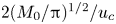 $2(M_0/{\rm \pi} )^{1/2}/u_c$ in (2.3) and (2.4), and then integrating gives an expression for the centreline velocity,
 $u_c$, as it depends upon distance,
 $x$, from the point source (virtual) origin:
 \begin{equation} u_c(x) = \xi_0 \frac{M_0^{1/2}}{x} . \end{equation}
In (2.8), the non-dimensional constant
 \begin{equation} \xi_0\equiv \frac{1}{\sqrt{\rm \pi}\,\alpha_g} \end{equation}
is an empirical parameter replacing the role of  $\alpha _g$. The corresponding jet radius is predicted to increase linearly with distance from the virtual origin as
 \begin{equation} b(x) = \frac{2}{\sqrt{\rm \pi}\xi_0} x. \end{equation}
While (2.8) gives the flow within a statistically steady turbulent jet, it is expected that the advance of the front of a starting jet should have the same dimensional dependence upon  $M_0^{1/2}/x$. Because the jet is injected continuously, the front is not influenced by strong vortex ring formation and it is considered to be quasi-steady after undergoing initial adjustments (Gharib, Rambod & Shariff Reference Gharib, Rambod and Shariff1998). Following the approach of Bhamidipati & Woods (Reference Bhamidipati and Woods2017) in their study of vertically rising starting plumes, we assume the front position
 $x_f(t)$ satisfies
 $\textrm {d}x_f/\textrm {d}t = \xi _f M_0^{1/2}/x_f$, in which
 $\xi _f$ is a non-dimensional measure of the front velocity. Integrating and rearranging gives an expression for
 $\xi _f$:
 \begin{equation} \xi_f=\frac{x_f^2}{2M_0^{1/2}(t+t_0)}, \end{equation}
in which  $t_0$ represents the time required for the jet to attain a self-similar shape (Bhamidipati & Woods Reference Bhamidipati and Woods2017). We will show that, with the correct choice of
 $t_0$,
 $\xi _f$ is indeed nearly constant for sufficiently large
 $t$ irrespective of the flow and particle parameters. However, the scaling described above will not be appropriate at large distances when the vertical extent of the jet becomes a significant fraction of the total fluid depth, in which case the flow of the ambient fluid over and around the jet becomes non-negligible. In our experiments, the vertical extent of the jet is
 ${\simeq }3/4$ the total depth after propagating a distance from the source of
 $x\approx 40\ \textrm {cm}$ and
 $x\approx 60$ cm, respectively, for bottom slope angles of
 $0^{\circ }$ and
 $8^{\circ }$. Most of our analyses of jet spreading and sediment deposition are well within this range of
 $x$.
2.2. Sedimentation
To derive a simple model for predicting the onset of sedimentation from a particle-bearing jet, we suppose that the particles are homogeneously spread within the vertical cross-section of the jet and they begin to settle out when the Gaussian profile of the jet speed near the bottom becomes comparable to the particle settling velocity,  $w_p$. Setting
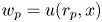 $w_p=u(r_p,x)$ in (2.1) thus gives an implicit formula for the critical radius
 $r_p(x)$ which is defined as the distance from
 $y = 0$ in the horizontal plane at which particles settle. Explicitly,
 \begin{equation} r_p(x) = \frac{2}{\sqrt{\rm \pi}} \frac{x} {\xi_0} \left[\ln\left(\xi_0 \frac{L_p}{x}\right)\right]^{1/2}, \end{equation}
in which we have used (2.8) and (2.10) along with the momentum-settling length scale  $L_p$, which is defined to be (Ernst et al. Reference Ernst, Sparks, Carey and Bursik1996)
 \begin{equation} L_p \equiv \frac{M_0^{1/2}}{w_p}. \end{equation}
In (2.12),  $x$ is bounded above by
 $\xi _0 L_p$, representing the maximum distance from the virtual origin beyond which particle settling must occur.
While (2.12) may be representative of where particles first descend to the bottom, it is possible for the particles consequently to slide along the bottom as a consequence of stresses imposed by the overlying flow through a process known as bedload transport. Whether the stresses are sufficiently strong to advect the settled particles is determined by the Shields parameter (Shields Reference Shields1936), defined as
 \begin{equation} {Sh}=\frac{u^2}{g^\prime d_p}, \end{equation}
in which  $u$ is the local flow velocity far from the boundary,
 $d_p$ is the particle diameter and
 $g^\prime =(\rho _p-\rho )g/\rho$ is the reduced gravity. Bedload transport occurs if
 $u$ is sufficiently large that
 ${Sh}$ exceeds a critical value,
 ${Sh}_c$, of order unity. The critical velocity below which no bedload transport occurs is thus given by
 $({Sh}_c g^\prime d_p)^{1/2}$. Equating this with (2.1) and rearranging, as in (2.12), the prediction for the interior boundary of the sediment bed is given by
 \begin{equation} r_s(x) = \frac{2} {\sqrt{\rm \pi}} \frac{x} {\xi_0} \left[\ln\left(\xi_0 \frac{\gamma_s L_s}{x}\right)\right]^{1/2}, \end{equation}
in which
 \begin{equation} L_s\equiv {\left(\frac{M_0}{g^\prime d_p}\right)}^{1/2}. \end{equation}
For convenience, we have defined  $\gamma _s\equiv {Sh}_c^{-1/2}$, which is an empirical quantity to be determined from experiments.
In the above discussion, it was assumed the particles were much larger than the viscous boundary layer associated with the ambient flow passing over the bottom wall. If the particles are much smaller than the boundary layer depth,  $\delta \sim \nu /u$, in which
 $\nu$ is the kinematic viscosity, then the velocity of the flow acting on the particles is of order
 $u_\nu \sim d_p u/\delta = {Re}_f u$, in which
 \begin{equation} {Re}_f \equiv \frac{u d_p}{\nu} \end{equation}
is the Reynolds number based upon the local ambient flow speed. Consequently, the condition for bedload transport, given by 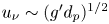 $u_\nu \sim (g^\prime d_p)^{1/2}$, can be recast in terms of
 $u$. Putting this expression in (2.14) gives the critical condition for bedload transport to be
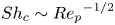 ${Sh}_c \sim {{Re}_p}^{-1/2}$ (Eames & Dalziel Reference Eames and Dalziel2000), in which
 \begin{equation} {Re}_p \equiv \frac{w_p d_p}{\nu} \end{equation}
is the particle Reynolds number. Recasting this critical condition in terms of the critical ambient flow speed,  $u_s$, outside the boundary layer gives
 \begin{equation} u_s = \frac{1}{\gamma_c} (g^\prime d_p)^{1/2}{{Re}_p}^{-1/4}, \end{equation}
in which  $\gamma _c$ is a non-dimensional empirical constant to be determined empirically. The location where particles ultimately sediment is therefore predicted to occur where
 $u_s=u(r,x)$. Rearranging, as in (2.12), we predict the sediment bed should begin to accumulate beyond a radius
 \begin{equation} r_c(x) = {\sqrt \frac{2}{\rm \pi}} \frac{x} {\xi_0} \left[\ln\left(\xi_0 \frac{\gamma_c L_c}{x}\right)\right]^{1/2}, \end{equation}
in which
 \begin{equation} L_c\equiv \frac{M_0^{1/2}}{u_s} . \end{equation}
If  ${Re}_p\ll 1$,
 $w_p$ is given by the Stokes settling formula, in which case
 $L_c = [(M_0^2 d_p)/(18 g^\prime \nu ^2)]^{1/4}$. For our experiments, in which
 ${Re}_p$ ranges between
 $0.5$ and
 $8$, we use the empirical formulae equations (24), (25) and (37) of Brown & Lawler (Reference Brown and Lawler2003), which account for the correction to the Stokes settling velocity due to particle inertia at these moderate particle Reynolds numbers.
The above equations, (2.12), (2.15) and (2.20), defining the inner boundary of the sediment bed will be compared below with experiment results to determine, respectively, if bedload transport is not important or, if it is important, whether the boundary layer has negligible influence on bedload transport ( ${Re}_f\gg 1$) or if it is significant (
 ${Re}_f\ll 1$).
3. Experimental set-up and analysis methods
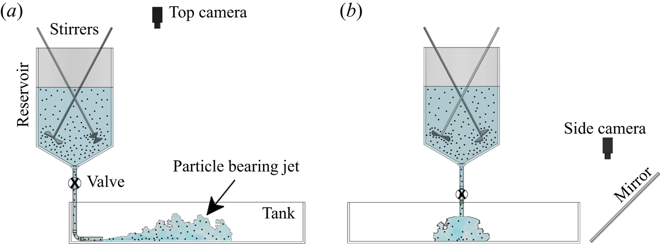
Here we describe the apparatus used for performing the experiments along with the techniques used for data analysis. A schematic of the experimental set-up is shown in figure 1.
Schematic of the experimental set-up showing (a) the side view and (b) the front view with the jet approaching the viewer.

3.1. Apparatus
The experiments were performed in a tank with length  $L_T=120$ cm, width
 $W_T =120$ cm and height
 $H_T = 30$ cm. This was suspended above the floor by four supports at the corners. In some experiments, the two supports were higher at the rear of the tank such that it sloped downward at a prescribed angle
 $\beta =8^\circ$ to the horizontal. A nozzle with diameter
 $d=1$ cm was positioned at the mid-span of the tank with its opening parallel to the bottom, situated 35 cm from the rear end of the tank. The nozzle consisted of an expansion chamber that led to a fine mesh covering a 0.2 cm radius opening. This set-up ensured turbulent flow exited the nozzle (Hunt & Linden Reference Hunt and Linden2001). Leading to the nozzle was 1 cm inner diameter flexible Tygon tubing connected to a hopper-shaped reservoir. This was a cylinder of height
 $H_R = 50\ \textrm {cm}$ and radius
 $R = 15\ \textrm {cm}$ which had a conical bottom sloping at an angle of
 $30^\circ$ to an opening at the bottom. Two angled mixers were situated inside the reservoir to ensure sufficient turbulent motion to keep particles in uniform suspension before and during an experiment. The hose itself passed through a valve, which was opened at the start of an experiment, and a clamp which was used to adjust the source volume flux,
 $Q_0$, leaving the nozzle. Tap water was put into both the tank and reservoir such that the maximum depth of water in the tank was 15 cm and the depth of water in the reservoir was 25 cm. With the base of the reservoir being situated 100 cm above the location of the nozzle, the flow was driven by near-constant pressure: during the course of an experiment, the depth of fluid in the reservoir decreased by no more than 1 cm for a total change in distance between the reservoir surface and nozzle of less than 1 %.
Shortly before the start of an experiment, the mixers in the reservoir were turned on, and 10 ml of blue food colouring was added. Then a pre-measured mass of glass ballotini, having density  $\rho _p = 2.5 \ {\textrm {g}}\ {\textrm {cm}}^{-3}$, was added to the reservoir. Depending upon the experiment, the spheres had mean diameters of
 $d_p\approx 88 \pm 10$,
 $120\pm 30$ or
 $212\pm 40\ \mathrm {\mu }{\textrm {m}}$. From the mass and size of the spheres and the known volume of fluid initially in the reservoir, the volume fraction of particles in the fluid,
 $\phi _v$, was determined. To ensure that the particles had negligible influence upon buoyancy in the jet, all experiments had
 $\phi _v\leqslant 0.01$. The typical Reynolds number of the jet at the source ranged from 4500 to 9000 in all the experiments.
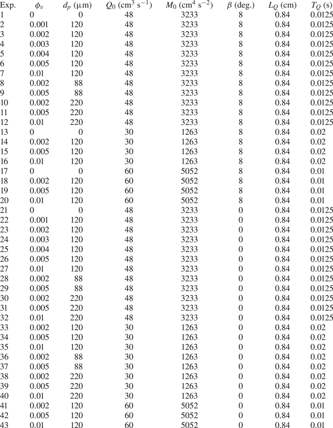
A list of all the experiments performed with corresponding parameters presented in this study is given in table 1. Several runs were repeated two to three times as a check of the consistency of results.
Source parameters for all the experiments: experiment number (Exp.), particle volume fraction ( $\phi _v$), particle diameter (
 $d_p$), volume flux (
 $Q_0$), momentum flux (
 $M_0$) and corresponding calculated jet length scale,
 $L_Q$, and time scale,
 $T_Q$.

At the start of an experiment, the valve was opened resulting in the release of a particle-bearing jet in the tank. When the jet front reached the front of the tank, the valve was closed, and the experiment ended. The average run time of the experiments lasted from 10 to 40 s depending upon  $Q_0$. In some experiments, red dye was impulsively injected into the tubing connecting the reservoir to the nozzle. This was done in order to distinguish the flow within the jet from the velocity at its front.
In order to visualize and record top views of the experiments, a light-emitting diode panel was situated underneath the tank and a digital camera (Canon Rebel T3i) situated 185 cm above the centre of the tank was directed vertically downward. Simultaneously, a second camera (Canon Rebel T5i) was positioned to look downward 50 cm above an angled mirror to give a side view of the experiment. Both cameras captured images at a rate of 24 frames per second with a resolution of  ${\approx }11\ \textrm {px}\,\textrm {cm}^{-1}$.
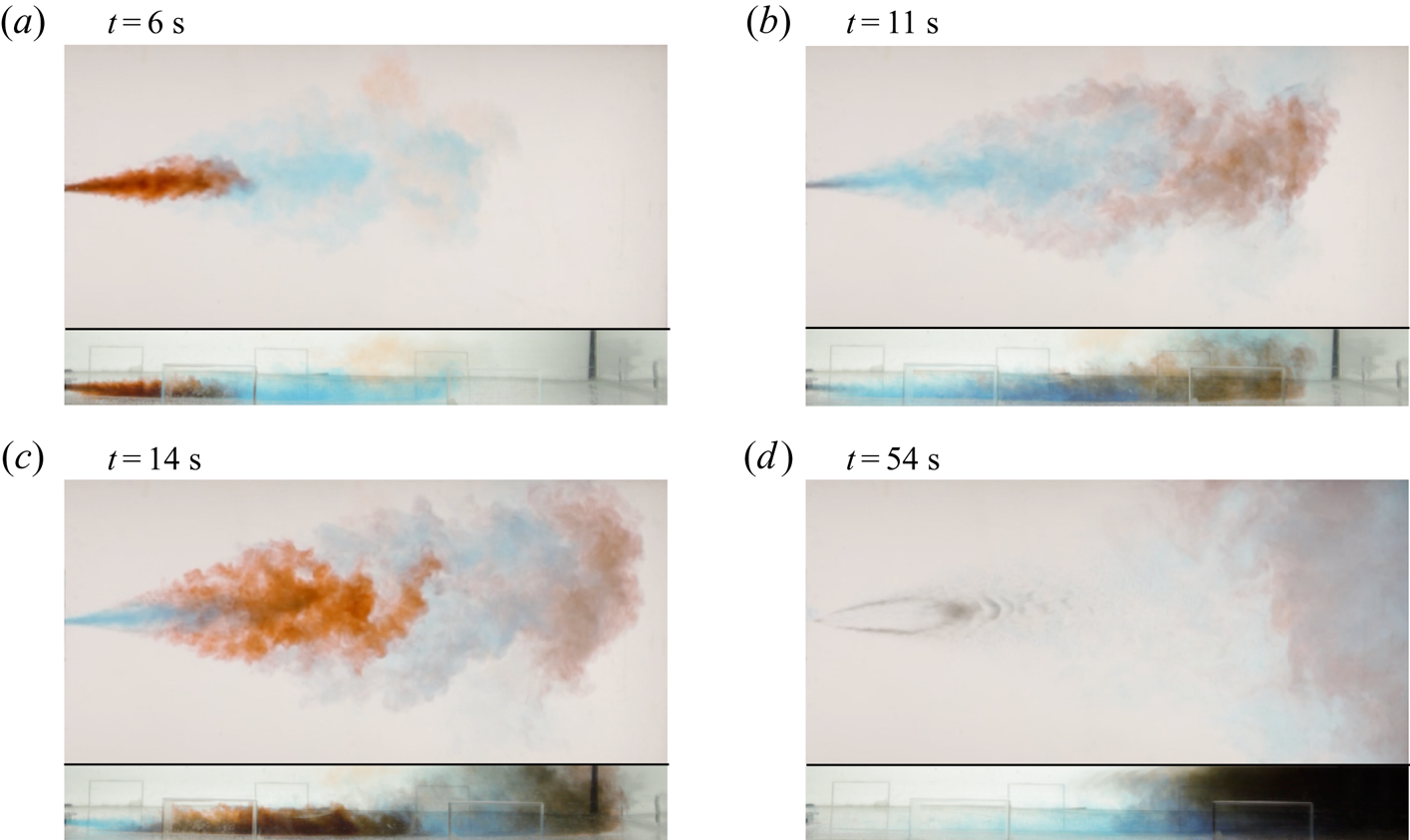
Images from a typical experiment are shown in figure 2. The side views show that the jet emanating from the nozzle touches the tank bottom shortly after exiting the nozzle. The top of the jet lies well below the free surface up to 80 cm from the nozzle. This is relevant because most sediments are deposited well before this distance indicating that the finite depth has little influence upon the deposition process, although we will show that it does influence entrainment into the jet far downstream of the source.
Top-view (upper image of each panel) and side-view (lower image of each panel) snapshots of Experiment 23 with  $Q_0 = 48\ {\textrm {cm}}^{3}\ {\textrm {s}}^{-1}$,
 $\phi _v=0.002$,
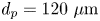 $d_p = 120\ \mathrm {\mu }{\textrm {m}}$ and
 $\beta =0^{\circ }$ shown at (a–d) four times as indicated. Red dye is impulsively injected into the hose leading to the nozzle shortly before 6 and 14 s. The image at 54 s shows the teardrop-shaped sediment deposit near the nozzle 10 s after the valve is closed. Snapshot dimensions:
 $\text {length} = 83\ \textrm {cm}$,
 $\text {width} = 40\ \textrm {cm}$ (top view) and
 $\text {height} = 10\ \textrm {cm}$ (side view).

For the experiment shown in figure 2, red dye was impulsively injected into the hose near the nozzle at two times after the experiment began. This clearly showed that fluid from the rear continuously reached the front of the blue-dyed jet before being swept sideways. A similar observation was made by Bhamidipati & Woods (Reference Bhamidipati and Woods2017) in their examination of vertically rising plumes. This effect could be attributed to the additional drag exerted on the front of the jet as it impinges upon a quiescent ambient fluid.
3.2. Analysis of jet
Digital movies from the top view of the experiments were processed using MatLab. To determine the position and shape of the blue-dyed jet front, for each frame of the recordings the image of the background in the absence of a jet was subtracted. The front and sides of the jet were then tracked by thresholding the image intensity to  $20\,\%$ of the maximum intensity value. In order to quantify the error in measurement of the front location,
 $x_f(t)$, different thresholding values were used, giving a location accuracy to within
 ${\pm }5\,\%$.
3.3. Light attenuation technique
Figure 2(d) shows a typical sediment pattern that formed after the end of an experiment. The teardrop shape of the sediment bed was observed for all the experiments.
The sediment depth was measured non-intrusively using the method of light attenuation (Munro & Dalziel Reference Munro and Dalziel2005; Sutherland & Hong Reference Sutherland and Hong2016). Because the particles were composed of glass spheres, light was scattered but not obstructed by the particles. Consequently, the light passing through the sediment is expected to decrease exponentially with the sediment depth,  $h$. Explicitly, the light intensity,
 $I$, is expected to depend upon
 $h$ as
 \begin{equation} I = I_b + (I_0-I_b)\,\textrm{e}^{-h/\sigma_h}. \end{equation}
This involves three empirically determined parameters:  $I_b$ is the effective ‘black’ intensity corresponding to a sediment depth so large that light no longer passes through it;
 $I_0$ is the intensity in the absence of particles; and
 $\sigma _h$ is the e-folding depth over which the intensity difference decreases by a factor e. The parameters were determined using a straight-edged scraper to make a linearly decreasing slope over a distance of 20 cm between a 1 cm tall guide and the bottom of a ‘calibration tank’. By recording the intensity of light passing through this uniform slope, a measurement of
 $I(h)$ was found. A nonlinear regression routine in MatLab was then used to determine a best-fit curve of the form (3.1). This procedure was followed for each of the three particle types. (See, for example, Sutherland & Hong (Reference Sutherland and Hong2016) for details of the calibration procedure.)
Once  $I_b$,
 $I_0$ and
 $\sigma _h$ were determined, it was straightforward to invert (3.1) to determine
 $h$ for given
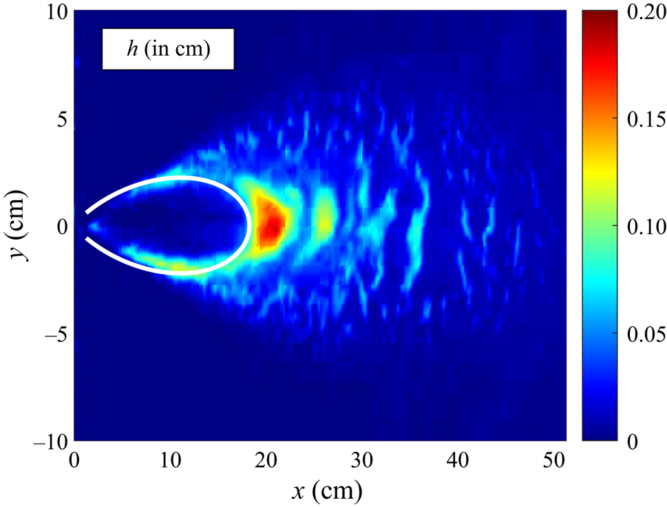
 $I$. As an example, figure 3 shows the measured sediment depth corresponding to Experiment 6.
Depth of the sediment deposit computed at the end of Experiment 6, which has  $\phi _v=0.5$ % and
 $d_p=120\ \mathrm {\mu }{\textrm {m}}$. The superimposed curve shows the predicted onset of sediment deposition according to (2.15), which includes the effect of bedload transport for
 ${Re}_f\gg 1$.

4. Quantitative results
4.1. Bulk dynamics
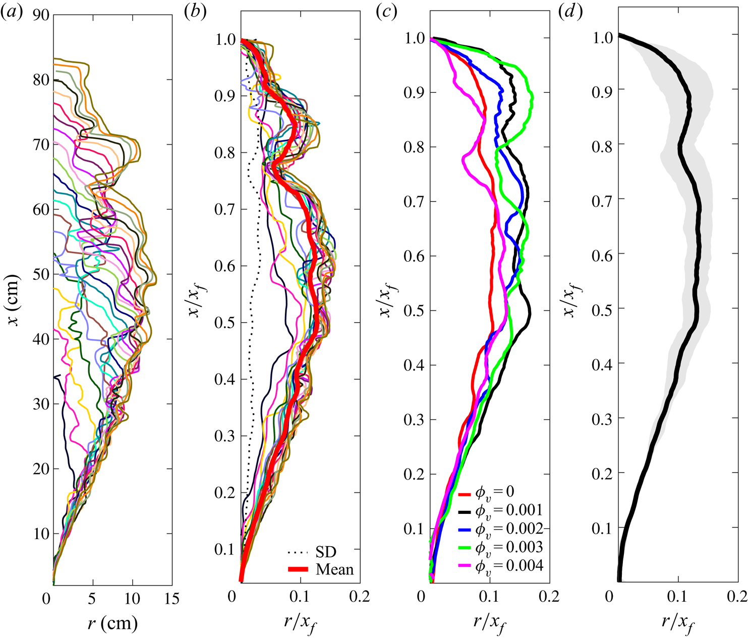
Figure 4(a) shows the outline of the jet at successive times as it advances and spreads laterally. Normalizing both the along-jet distance,  $x$, and radial distance,
 $r$, with the front position,
 $x_f$, leads to an approximately self-similar profile (figure 4b). These scaled profiles are then averaged to produce plots of the mean relative spread of the current with relative distance from the source. Figure 4(c) plots these mean profiles computed for experiments of jets with different particle concentrations,
 $\phi _v$. As expected for particle-bearing (not particle-laden) jets, the profiles effectively overlap, indicating that the particles have negligible influence upon the jet evolution. Taking the radial mean of all these profiles for each
 $x$ gives the self-similar jet profile plotted in figure 4(d). The standard deviation about the mean becomes large only near the front of the jet where greater fluctuations occur as a consequence of the impinging head interacting with the ambient fluid and due to recirculation patterns occurring in the lee of the head, where the fluid in the jet catches up to the front and then spreads laterally, as shown in figure 2.
From Experiment 5, (a) lateral extent of the jet as a function of along-jet coordinate  $x$ plotted at
 $\text {time steps}=0.5\ \textrm {s}$ starting from
 $t = 2\ \textrm {s}$, (b) corresponding lateral extent with along-jet coordinate scaled by the front position
 $x_f$, (c) average (solid lines) of the scaled front positions from Experiments 1, 2, 3, 4 and 5 with different particle concentrations
 $\phi _v$, having fixed
 $Q_0=48\ {\textrm {cm}}^{3}\ {\textrm {s}}^{-1}$,
 $d_p=120\ \mathrm {\mu }{\textrm {m}}$ and
 $\beta =8^{\circ }$ and (d) mean profile (line) and standard deviation (grey shaded region) computed from Experiments 1, 2, 3, 4 and 5.

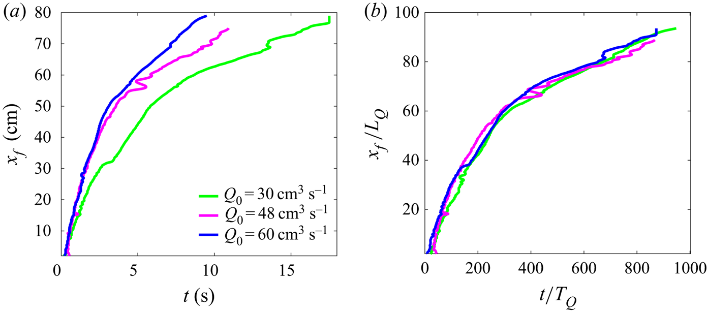
As well as having a self-similar shape, the advance of the jet front is self-similar in time. This is shown in figure 5, which plots the front position of the jet in time from experiments with different values of  $Q_0$. Upon non-dimensionalizing position and time, respectively, with the characteristic scales
 $L_Q$ and
 $T_Q$, the curves collapse well, as shown in figure 5(b).
(a) Front position,  $x_f$, versus time for three different
 $Q_0$ with
 $\phi _v = 0$ and
 $\beta = 8^{\circ }$. (b) Scaling with jet length scale
 $(L_Q)$ and time scale
 $(T_Q)$.

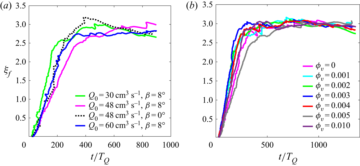
A more quantitative representation of the self-similarity of the front position is given by plots of the non-dimensional velocity,  $\xi _f$, defined by (2.11), as shown in figure 6. With suitable choice of the virtual origin time (
 $t_0$), which accounts for the adjustment of the jet front to self-similar form upon leaving the nozzle, the values of
 $\xi _f$ are found to be constant after sufficient time. For
 $Q_0=48\ {\textrm {cm}}^{3}\ {\textrm {s}}^{-1}$, typical values of
 $t_0$ lie in the range 2–6 s. The corresponding non-dimensional front velocity
 $\xi _f$ in our experiments was found to be
 $\xi _f\simeq 2.8\pm 0.2$ which is moderately higher than the value
 $\xi _f\simeq 1.99\pm 0.06$ measured for plumes (Bhamidipati & Woods Reference Bhamidipati and Woods2017). As expected,
 $\xi _f$ is not dependent upon the particle concentration
 $\phi _v$, volume flux
 $Q_0$ or slope angle
 $\beta$.
(a) Non-dimensional velocity ( $\xi _f$) defined by (2.11) corresponding to the scaled time (
 $t/T_{Q}$) for different
 $Q_0$ and
 $\beta$ with
 $\phi _v = 0.005$ and
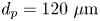 $d_p = 120\ \mathrm {\mu }{\textrm {m}}$. (b) Variation of
 $\xi _f$ for different
 $\phi _v$ with
 $Q_0 = 48 \ {\textrm {cm}}^{3}\ {\textrm {s}}^{-1}$,
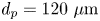 $d_p = 120\ \mathrm {\mu }{\textrm {m}}$ and
 $\beta = 8^{\circ }$.

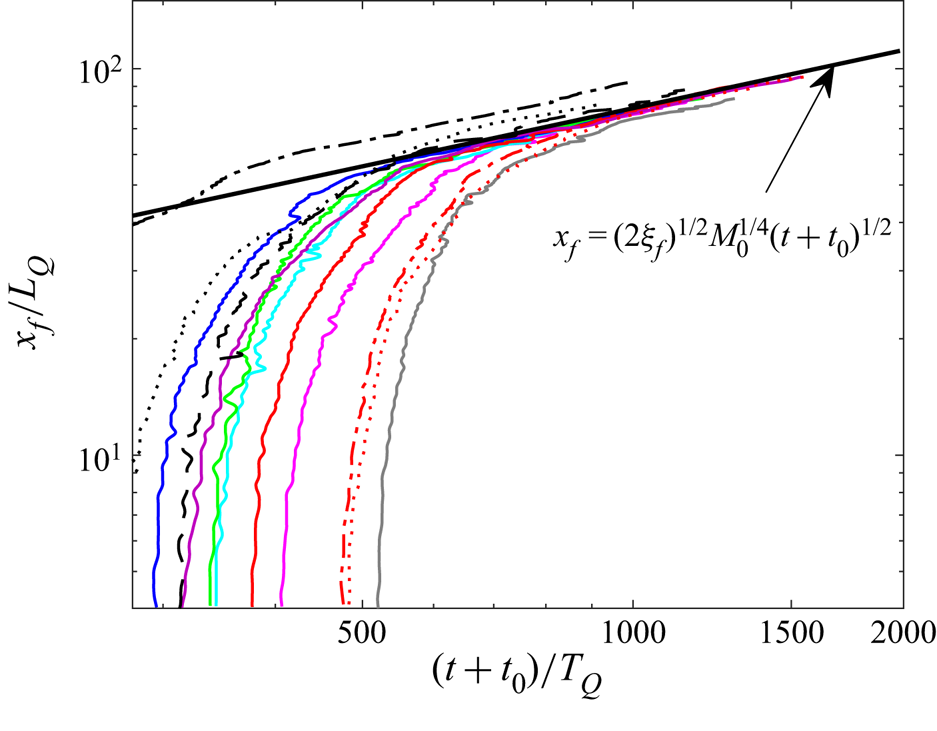
Making use of the virtual time,  $t_0$, to become self-similar, figure 7 plots the front position, scaled with
 $L_Q$, versus time with respect to the virtual time
 $t_0$, scaled by
 $T_Q$. For all experiments, these collapse to the semi-empirical prediction given by (2.11) at sufficiently large times.
Scaled front position as a function of scaled time for various experiments with different  $\phi _v$,
 $\beta$,
 $d_p$ and
 $Q_0$. All the solid curves correspond to varying
 $\phi _v$ and have the same parameters and colour scheme as that of figure 6(b). The black dotted and black dash-dotted lines correspond to
 $Q_0 = 30$ and
 $60\ {\textrm {cm}}^{3}\ {\textrm {s}}^{-1}$, respectively, with
 $\phi _v =0$ and
 $\beta = 8^{\circ }$. The red dotted and red dash-dotted lines correspond to
 $d_p = 88$ and
 $220\ \mathrm {\mu }{\textrm {m}}$, respectively, with
 $\phi _v =0.002$,
 $Q_0 = 48\ {\textrm {cm}}^{3}\ {\textrm {s}}^{-1}$,
 $\beta = 8^{\circ }$. The black dashed line corresponds to
 $\beta = 0^{\circ }$ with
 $Q_0 = 48 \ {\textrm {cm}}^{3}\ {\textrm {s}}^{-1}$ and
 $\phi _v = 0$. The solid black line represents the theoretical scaling law for the front position.

By examination of the motion of injected red dye relative to the front, as shown in figure 2, we found the velocity scaling of the steady jet to be given by  $\xi _0 \simeq 3.9 \pm 0.3$, so that
 $\xi _0\simeq 1.4\xi _f$. Although the front position plotted in figure 7 shows that the initial adjustment to self-similarity extends a considerable distance from the source, the flow in the lee of the front is found to be self-similar, as confirmed by tracking the motion of injected red dye. Using (2.9), the measured value of
 $\xi _0$ corresponds to an entrainment parameter
 $\alpha _g\simeq 0.14\pm 0.01$, which is more than twice the value typically measured for a free jet (Carazzo et al. Reference Carazzo, Kaminski and Tait2006). This result is surprising given that the entrainment of a wall jet is expected to be smaller than the entrainment parameter,
 $\alpha _g\simeq 0.05$, for a free jet due to the existence of a no-slip condition near the wall and the suppression of meandering that, in comparison with the free jet, should reduce the length of the turbulent/non-turbulent interface between the jet and ambient fluid (Parker et al. Reference Parker, Burridge, Partridge and Linden2020). This suggests that the finite depth of the ambient fluid may influence the entrainment process far from the source where the jet becomes self-similar, a consequence of the ambient fluid above the jet being directed back towards the source so that the total volume flux across a vertical-spanwise cross-section is always zero. Despite this discrepancy, it is anticipated that such a return flow has negligible influence upon sedimentation from the jet near the source, for which peak deposition occurs typically within
 $20\ \textrm {cm} \simeq 24 L_Q$ from the source.
4.2. Particle sedimentation
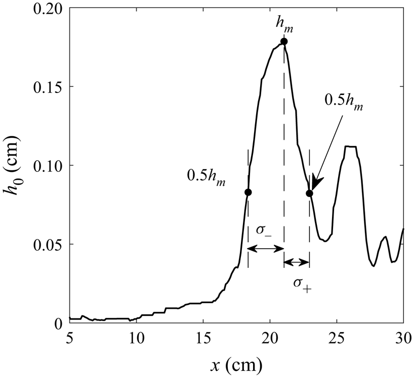
From measurements of the height of the sediment taken at the end of an experiment (see, for example, figure 3), we extract the height of the sediment along the centreline of the jet, as shown in figure 8. In all cases, the height exhibits a large peak sometimes followed by smaller peaks in its lee. The largest peak typically has width of the order of 2 cm with steeper slope in the lee.
Height distribution of the sediment along the jet centreline determined from Experiment 6.

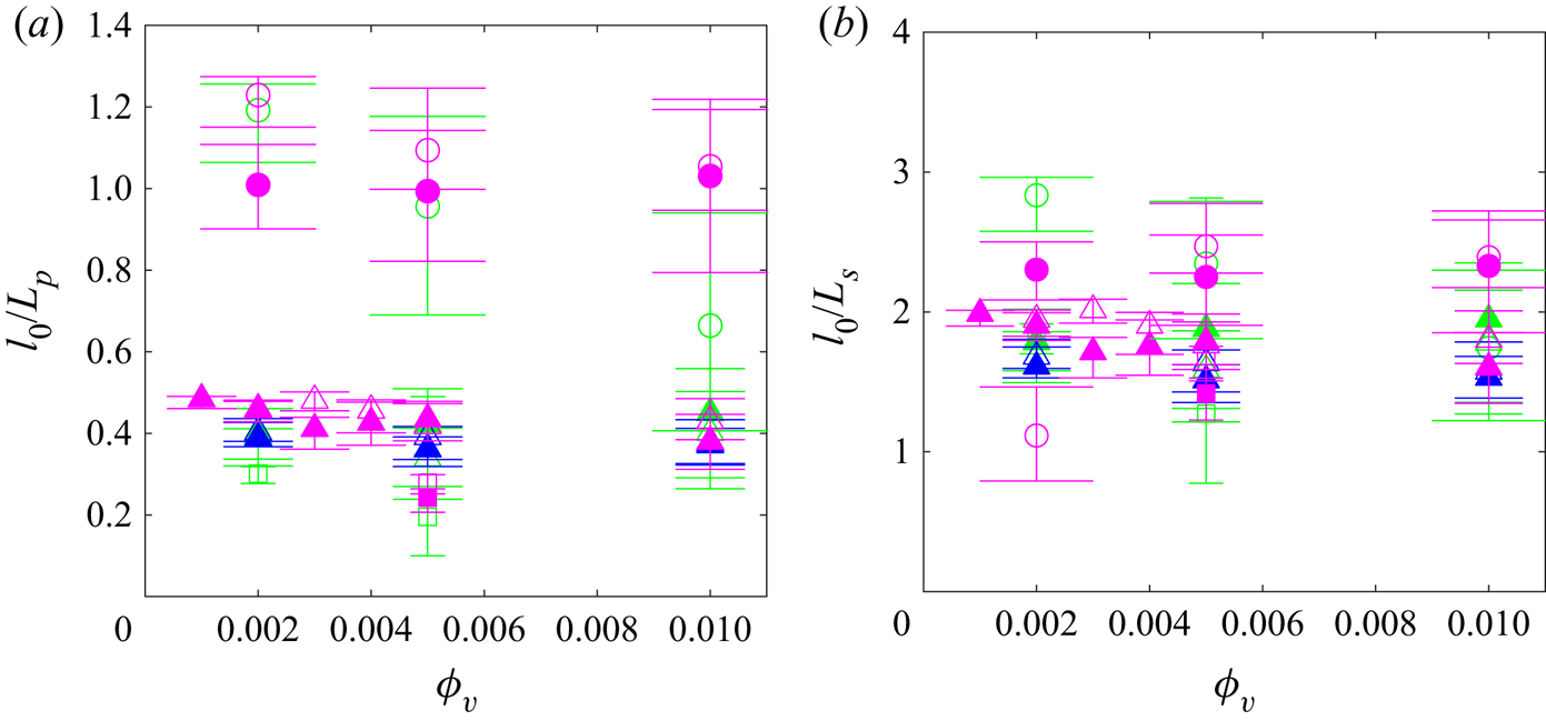
Generally, the distance,  $l_0$, from the virtual origin to the peak sediment depth is larger if the source momentum flux is larger. This is consistent with the estimates for the length scales of deposition,
 $L_p$,
 $L_s$ and
 $L_c$, respectively given by (2.13), (2.16) and (2.21). However, as shown in figure 9(a), when
 $l_0$ is scaled by
 $L_p$ (the length scale that assumes deposition with no consequent bedload transport), the results show a strong dependence upon the particle size. On the other hand, when
 $l_0$ is scaled by
 $L_s$ (which includes the influence of bedload transport after settling but neglects the influence of the viscous boundary layer), all the data collapse reasonably well to relative values of
 $l_0/L_s \simeq 1.8 \pm 0.4$ (figure 9b).
Distance,  $l_0$, from virtual origin of the maximum sediment depth measured from experiments for varying
 $\phi _v$,
 $d_p$ and
 $\beta$, given relative to scalings (a)
 $L_p$ and (b)
 $L_s$. Colour represents
 $Q_0$ as indicated in figure 5. Filled symbols (
 $d_p = 88\ \mathrm {\mu }{\textrm {m}}$, squares;
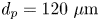 $d_p = 120\ \mathrm {\mu }{\textrm {m}}$, triangles;
 $d_p = 220\ \mathrm {\mu }{\textrm {m}}$, circles) for
 $\beta = 8^{\circ }$. Open symbols (
 $d_p = 88\ \mathrm {\mu }{\textrm {m}}$, squares;
 $d_p = 120\ \mathrm {\mu }{\textrm {m}}$, triangles;
 $d_p = 220\ \mathrm {\mu }{\textrm {m}}$, circles) for
 $\beta = 0^{\circ }$. Vertical bars indicate upstream half-width (
 $\sigma _{-}$) and downstream half-width (
 $\sigma _{+}$) as indicated in figure 8.

A similar good collapse of data occurs in plots of  $l_0/L_c \simeq 1.4 \pm 0.2$ (not shown). However, when the flow Reynolds number (2.17) is computed using
 $u=u_c(L_c)$, we find
 ${Re}_f\gg 1$. Hence the viscous boundary layer should not play a significant role in determining the critical Shields parameter.
We define  $l_s$ to be the along-jet distance from the virtual origin to where the sediment bed first appears. From measurements of
 $l_s$, we construct the ratio
 $l_s/L_s$, and so determine the value of the empirical constant
 $\gamma _s$ appearing in (2.15) to be
 $\gamma _s = l_s/(\xi _0 L_s) \simeq 0.33 \pm 0.11$. The measured value of
 $\gamma _s$ is used in (2.15) to predict the spanwise radius as a function of along-stream distance from the virtual origin where particles first sediment. In particular, this curve is superimposed on the plot of sediment depth in figure 3, showing good agreement to the location where sediment depth first becomes non-zero inside the teardrop-shaped deposit.
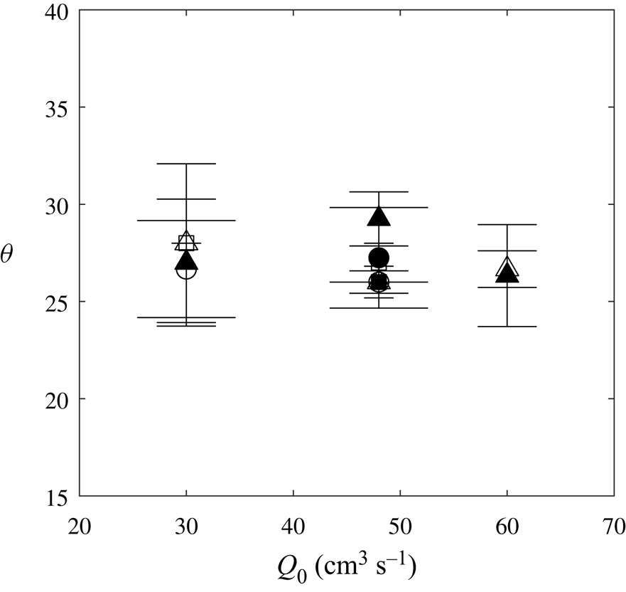
Near the source, the sediments deposit along lines at a near-constant angle from the source. The particles settle when the mean velocities at the periphery of the jet become sufficiently slow compared with the particle settling velocity. The measured angles of the sediment deposit determined from experiments with various  $Q_0$,
 $\beta$ and
 $d_p$ are shown in figure 10. The angles are measured from the inside of the teardrop-shaped sediment bed. For each point, the error bars indicate the deviation for
 $\phi _v$ in the range of
 $0.1\,\%$ to
 $1\,\%$. In all cases the angle ranges between
 $25^\circ$ and
 $30^\circ$.
Sediment deposit angles ( $\theta$, in degrees) for different
 $Q_0$. Symbols indicate the particle diameter, with
 $d_p=88\ \mathrm {\mu }{\textrm {m}}$ (
 $\blacksquare$),
 $120\ \mathrm {\mu }{\textrm {m}}$ (
 $\blacktriangle$) and
 $220\ \mathrm {\mu }{\textrm {m}}$ (
 ). Filled (open) symbols correspond to
 $\beta = 8^{\circ }$ (
 $0^{\circ }$). Bars represent the standard deviation computed for measurements over all
 $\phi _v$ values with fixed
 $Q_0$,
 $d_p$ and
 $\beta$.

In order to estimate the height scale determining the maximum sediment depth,  $h_m$, we note that the volume of particles injected during the time
 $t_f$ of an experiment is given by
 $V=Q_0t_f\phi _v$. The particles are assumed to settle in a teardrop shape bounded inside by the curve given by (2.15) with
 $\gamma _s=0.33$, and bounded outside by the same curve but with
 $\gamma _s=1$, representing the condition that the kinetic energy of the flow is insufficient to overcome the potential energy of the particles. The basal area of this curve is given by
 \begin{equation} A= 2\sqrt{\frac{2}{\rm \pi}} I \xi_0 (1-\gamma_s^2) L_s^2, \end{equation}
in which  $I=\int _0^1 x [\ln (1/x)]^{1/2}\,{\textrm {d}x} \simeq 0.313$. Thus, assuming a loose-sphere packing fraction of
 $p_f=0.56$, and evaluating the constants in (4.1), the mean height is predicted to be
 \begin{equation} H_s = \frac{1}{p_f}\frac{V}{A} \simeq (1.0 \pm 0.1) \frac{Q_0 t_f\phi_v}{L_s^2}. \end{equation}
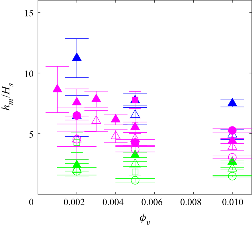
As a test of the predicted height scale (4.2), figure 11 plots the measured values of the maximum height,  $h_m$, normalized by
 $H_s$. As the maximum height is expected to exceed the mean, the figure shows that
 $H_s$ correctly captures the order of magnitude of the expected mean sediment depth. However, there is clearly a trend such that the relative maximum depth is lower if the source volume (hence momentum) flux is smaller. For these experiments, the width of the sediment bed about the primary peak was found to be longer. This suggests that additional consideration should be made for the piling up of the sediment in front of the impinging jet and the influence of the bed morphology upon the jet itself near the lower boundary. Consideration of such dynamics lies beyond the scope of this study.


5. Conclusion
In this paper the spreading and sedimentation dynamics of horizontal and bottom-sloping dispersed particle-bearing jets in uniform ambient fluid were studied experimentally for a range of parameters, namely the particle volume fraction  $\phi _v$, source volume flux
 $Q_0$, particle diameter
 $d_p$ and slope angle
 $\beta$. Our results show that irrespective of these parameters, the propagation of the jet front follows a self-similar behaviour. The relation between front position with time was found to be
 $x_f = (2\xi _f (t+t_0))^{1/2} M_0^{1/4}$ with
 $\xi _f\simeq 2.8\pm 0.2$ and
 $t_0=4 \pm 2$ s. The flow in the steady jet behind the front advanced towards the front such that the non-dimensional velocity was
 $\xi _0\simeq 1.4\xi _f$. The magnitudes of
 $\xi _f$ and
 $\xi _0$ are larger than anticipated for an unbounded jet, suggesting that the finite depth of the ambient fluid influences entrainment and the jet speed far downstream of the source where the jet width is a non-negligible fraction of the total depth. Near the source where sediment deposition occurs the jet width is considered to be sufficiently small that finite-depth effects should not play a role in sedimentation.
Supposing that the radial profile of the jet assumes a Gaussian structure, a prediction was made for the momentum-settling length scale,  $L_p$, at which the particle settling velocity exceeds the mean turbulent flow speed. This provided a poor collapse of data. However, the prediction for the extent of the sediment bed improved on using the length scale
 $L_s$, which accounted for the bedload transport of particles after they settle out of the jet, neglecting viscous boundary layer dynamics. The observed teardrop-shaped structure of the sediment bed was well predicted using the bedload theory by choosing an empirical parameter
 $\gamma _s\simeq 0.33\pm 0.11$ such that the maximum distance before settling begins was found to be
 $l_s=\gamma _s\xi _0 L_s$. On the other hand, the maximum height, when scaled by the corresponding mean height
 $H_s$, showed that the relative height was steeper and the peak more narrow if the jet momentum at the source was larger. Because the theory for the run-out length
 $l_s$ already accounted for the decrease in the maximum jet velocity with distance from the source, it is believed that the dependence of
 $h_m/H_s$ upon
 $Q_0$ and
 $M_0$ should also account for the influence of the growing sediment bed upon the jet itself. This will be the focus of future work.
Acknowledgements
We thank the Shastri Indo-Canadian Institute for providing financial support for this research work in the form of a Shastri Institutional Collaborative Research Grant (SICRG). We are grateful to the anonymous reviewers for giving insightful comments on this work.
Declaration of interests
The authors report no conflict of interest.