1. Introduction
Particle-in-cell (PIC) codes are known for their versatility and relative speed. They are used to simulate a wide range of phenomena in kinetic and collisionless (or weakly collisional) plasma physics. To solve Maxwell equations, many of them use the finite-difference time-domain method first proposed by Yee (Reference Yee1966), a simple second-order method easily parallelisable but suffering from some numerical dispersion error which gives rise to what is known as numerical Cherenkov radiation (NCR) (Godfrey Reference Godfrey1974). There has been much work in recent years proposing different ways to limit the impact of NCR (Lehe et al. Reference Lehe, Lifschitz, Thaury, Malka and Davoine2013; Xu et al. Reference Xu, Yu, Martins, Tsung, Decyk, Vieira, Fonseca, Lu, Silva and Mori2013; Godfrey & Vay Reference Godfrey and Vay2014; Yu et al. Reference Yu, Xu, Decyk, Fiuza, Vieira, Tsung, Fonseca, Lu, Silva and Mori2015; Lehe et al. Reference Lehe, Kirchen, Godfrey, Maier and Vay2016; Li et al. Reference Li, Yu, Xu, Fiuza, Decyk, Dalichaouch, Davidson, Tableman, An and Tsung2017, Reference Li, Miller, Xu, Tsung, Decyk, An, Fonseca and Mori2021). We recently proposed a novel approach to mitigate the effects of this numerical artefact through the modification of the field interpolation (Bourgeois & Davoine Reference Bourgeois and Davoine2020).
This new technique, which we called B-TIS for B-translated interpolation scheme, is easy to implement in most PIC codes using the Yee scheme, has negligible impact on performance or communications and showed good results to reduce the impact of NCR in laser wakefield acceleration (LWFA) simulations, but we believe it could also help to improve the modellisation of laser–particle interaction in a number of cases.
One domain where this interaction is particularly important, and thus could benefit greatly from such improvements, is the simulation of vacuum laser acceleration (VLA): where a laser beam directly interacts with electrons propagating in a vacuum to accelerate them (Esarey, Sprangle & Krall Reference Esarey, Sprangle and Krall1995; Quesnel & Mora Reference Quesnel and Mora1998; Yu et al. Reference Yu, Yu, Ma, Sheng, Zhang, Daido, Liu, Xu and Li2000; Cline et al. Reference Cline, Shao, Ding, Ho, Kong and Wang2013; Varin et al. Reference Varin, Payeur, Marceau, Fourmaux, April, Schmidt, Fortin, Thiré, Brabec and Légaré2013). Though it is a difficult technique to set up experimentally, it benefits from the extremely strong fields of the laser pulse (a few ${\rm TV}\,{\rm m}^{-1}$ ) which makes it a good candidate to produce MeV electrons at high repetition rate (Marceau et al. Reference Marceau, Hogan-Lamarre, Brabec, Piché and Varin2015; Carbajo et al. Reference Carbajo, Nanni, Wong, Moriena, Keathley, Laurent, Miller and Kärtner2016).
B-TIS allows for a better modellisation of laser–electron interaction by reducing the error on the computed magnetic field which in turn leads to more accurate Lorentz force and particle motion. The improvement is especially significant for electromagnetic fields propagating at $c$ along the electron acceleration axis. The study of VLA thus appears as a logical next step as it fits well within the limitations of B-TIS and provides a good benchmark to investigate the reproduction of the physical phenomena at play in laser–electron interaction. This should also help to improve the modellisation of the direct laser acceleration (DLA) regime appearing in LWFA which presents great similarities to VLA (Pukhov, Sheng & Vehn Reference Pukhov, Sheng and ter Vehn1999; Shaw et al. Reference Shaw, Tsung, Vafaei-Najafabadi, Marsh, Lemos, Mori and Joshi2014, Reference Shaw, Lemos, Amorim, Vafaei-Najafabadi, Marsh, Tsung, Mori and Joshi2017; Zhang, Khudik & Shvets Reference Zhang, Khudik and Shvets2015).
In this article, we start in § 2 with the study of a single electron interacting with a plane wave so as to compare and validate the simulation results against a simple analytical model. This simple study highlights the limitations of the different simulation techniques available and prompted us to develop an improved version of B-TIS that should be even more robust and accurate than the previous one. In § 3 we see how the Gaussian shape of a laser pulse impacts those results before, in § 4, looking into the acceleration of a bunch of electrons by a laser beam and finally the application of our results to a case of DLA in a LWFA simulation.
2. Electron dynamic in an electromagnetic plane wave
We first study the case of a single electron interacting with a propagating plane wave. This simple situation can be analytically modelled which gives us a useful benchmark to evaluate the accuracy of our numerical simulations.
2.1. Analytical model
Considering one electron in a vacuum, we can write its motion equation in terms of the electromagnetic vector potential $\boldsymbol {A}$ as

where $\boldsymbol {p}$ is the electron momentum, $\boldsymbol {v}$
 its velocity, $e$
 the elementary charge and the scalar potential $\phi = 0$
 .
For a plane wave propagating along the $x$ axis, the vector potential depends only on $x$
 and is polarised in the $yz$
 plane. Assuming an electron initially at rest, we thus get to


with $\boldsymbol {p}_\perp = p_y \boldsymbol {e_y} + p_z \boldsymbol {e_z}$ , $m_e$
 being the electron mass and $\gamma$
 its Lorentz factor. We can recognise in (2.2) the expression for the relativist ponderomotive force in the one-dimensional case.
From the conservation of energy equation for the electron and using the fact that for a plane wave propagating at $c$ along the $x$
 axis, $( {\partial }/{\partial t} + c ({\partial }/{\partial }x) ) A = 0$
 , we can then show that the quantity $\gamma - p_x / m_e c$
 is conserved. With the electron being initially at rest, we have $\gamma (t=0)=\gamma _0=1$
 and $p_x(t=0)=p_{x,0}=0$
 which leads to

We thus have three equations describing the dynamic of an initially at rest electron in a propagating plane wave:


2.2. Numerical simulations
All numerical simulations presented in this article were performed using the code Calder (Lefebvre et al. Reference Lefebvre, Cochet, Fritzler, Malka, Aléonard, Chemin, Darbon, Disdier, Faure and Fedotoff2003). Before we delve into the results of those simulations though, we first discuss the computation of electromagnetic fields and their resulting actions in PIC codes in order to introduce and summarise the B-TIS method proposed in Bourgeois & Davoine (Reference Bourgeois and Davoine2020).
2.2.1. Temporal interpolation of the magnetic field $B$ in PIC codes

2.2.1.1. Standard temporal interpolation
Although there have been interesting new developments to create dispersionless Maxwell solvers in recent years, notably most recently (Pukhov Reference Pukhov2020), Calder, as many other PIC codes, still uses the simple and robust finite-difference time-domain Yee scheme (Yee Reference Yee1966) to solve the Maxwell equations. Electric ($E$ ) and magnetic ($B$
 ) fields are thus calculated using a leap-frog method: they are defined on different grids which are offset spatially by half a cell but also temporally by $\Delta t / 2$
 .
Let us consider the computation of the transverse Lorentz force applied to a moving particle in our simulation. The particle can move freely in the whole simulated space while the fields are computed only on specific grid points. It is thus necessary to interpolate the electromagnetic fields onto the charged particle position to calculate its motion.
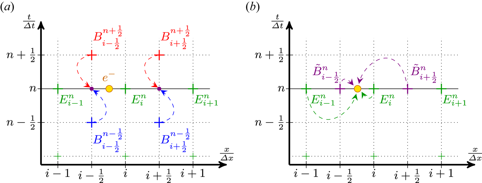
This simple situation, with the field amplitude values known on the different points of the grid and an electron moving freely between those points, is shown in figure 1 for a simple one-dimensional grid. Considering only the longitudinal dimension $x$ to simplify the notations, $A^{n}_{i}$
 then denotes the value of the field $A$
 at the $n$
 th time step and the $i$
 th point of the spatial grid or in other terms $A^{n}_{i}= A (t= n\Delta t,x=i\Delta x )$
 . Due to the leap-frog nature of the Yee scheme, values of the $E_y$
 fields are known at integer time steps and grid points while values for $B_z$
 are known at half-integer time steps and grid points. In the remainder of this section, we only consider $E_y$
 and $B_z$
 – which are required to compute the transverse force $F_y$
 – and then omit the $y$
 and $z$
 indices when it is not absolutely necessary so as not to clutter the notation.
Usual interpolation process of electromagnetic fields on a one-dimensional spatial grid at the $n$ th time step in order to get the transverse force $F_y^n$
 applied on the particle represented by the yellow circle. (a) The initial configuration where the field values are known at different times and spatial points. The temporal interpolation to get $\tilde {B}^n$
 is shown with dashed arrows. (b) The subsequent spatial interpolation of $E^n$
 and $\tilde {B}^n$
 on the particle (again with dashed arrows and first order).

As the fields are initially not known at the same time step, a temporal interpolation is necessary to get $\tilde {B}^n$ before the spatial interpolation and the computation of the force which is done at the integer time step $n$
 . The simplest and most common method is the linear time interpolation (LTI) $\tilde {B}^n = ( B^{n-{1}/{2}} + B^{n+{1}/{2}} )/2$
 as is shown in figure 1(a) but a quadratic time interpolation (QTI), with

can sometimes be used instead for higher accuracy (Lehe et al. Reference Lehe, Thaury, Guillaume, Lifschitz and Malka2014). Once both fields $E$ and $B$
 are known at the same time step, they are interpolated spatially onto the particles. This step is shown in figure 1(b). Once again different kinds of spatial interpolation can be used with varying orders of interpolation. The one depicted here is, for simplicity's sake, a first-order method (linear interpolation).
2.2.1.2. Bypassing the need for a temporal interpolation: B-TIS
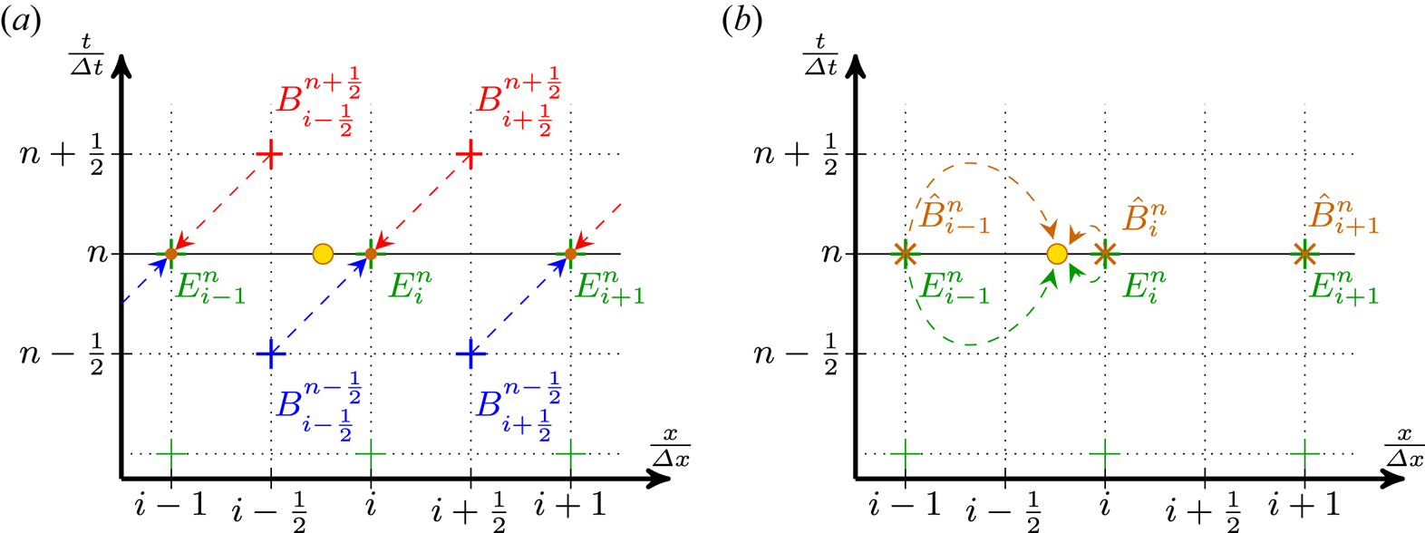
The idea behind our new scheme proposed in Bourgeois & Davoine (Reference Bourgeois and Davoine2020) is to simply use the available value of the magnetic field as the value we need. That is, interpolating the fields at the particle position using ($E_i^{n}$ , $\hat {B}_{i}^{n}= B_{i+{1}/{2}}^{n+{1}/{2}}$
 ) instead of ($E_i^{n}$
 , $\tilde {B}_{i+{1}/{2}}^{n}$
 ) as previously shown. Of course, doing so is only physically sound if $B_{i}^{n} \approx B_{i+{1}/{2}}^{n+{1}/{2}}$
 . Thankfully this condition means for a wave propagating at $c$
 that $B(x,t) \approx B(x+\Delta x/2, t + \Delta t/2)$
 which is true as long as $\Delta x \approx c \Delta t$
 . Although this last condition can be limited in the simulation by the Courant–Friedrichs–Lewy condition, it is usually verified in PIC simulations as having a ratio $\Delta x / \Delta t$
 close to $c$
 improves the quality of the results.
This new method effectively results in a translation of the calculated $B$ field before the spatial interpolation, hence its name: B-translated interpolation scheme. This process is described in figure 2.
Modified interpolation process of electromagnetic fields: B-TIS on a one-dimensional grid at the $n$ th time step. (a) The same initial configuration as figure 1(a) but instead of the temporal interpolation of $B$
 , the relation $\hat {B}^n_i = B^{n+{1}/{2}}_{i+{1}/{2}}$
 is used. (b) The result of this translation and the subsequent spatial interpolation of $E^n$
 and $\hat {B}^n_i$
 on a particle.

2.2.1.3. Computational error introduced
Both approaches introduce an error on the computed values of the magnetic field compared with an ideal situation where the magnetic field can be computed at integer time steps.
Let us consider a given magnetic field $B(\varphi ) = B_0 \cos (\varphi )$ . The computation of the numerical value of that field in the simulation introduces an error $\varepsilon$
 which depends on the method used:


with $\varphi = k_x x + k_y y + k_z z - \omega t$ , $\delta \varphi = {\omega \Delta t}/{2}$
 and $\widehat {\delta \varphi } = (k_x \Delta x - \omega \Delta t)/2$
 . Here $\omega$
 is the field's angular frequency and $k_x$
 , $k_y$
 , $k_z$
 its wavevector components.
For longitudinally propagating waves with $\omega /k_x \approx c$ and $c \Delta t \approx \Delta x$
 , $\widehat {\delta \varphi }$
 can become very small and the gain in accuracy should then be significant. This improvement of the computation of the magnetic field is what enables B-TIS to effectively suppress the effects of NCR. Indeed, the more accurate computation result in the induced Lorentz force, from the interaction of the NCR with particles, being negligible. In effect, the spurious radiation is still generated and present in the simulation but has no impact on the simulated particles.
2.2.2. Comparison of the different temporal interpolation methods
Three simulations were originally performed, each with a different temporal interpolation method introduced earlier: LTI, QTI and B-TIS. To reproduce in a two-dimensional simulation the situation presented above, we use a plane wave propagating along the $x$ axis, infinite in width along the $y$
 axis. Periodical boundary conditions are used on the longitudinal edges of the simulation box to recreate the infinite transverse property of the wave.
We chose the polarisation direction in the simulation plane (along the $y$ axis). The laser wavelength is $\lambda _0 = 2 {\rm \pi}c / \omega _0$
 , with $\omega _0$
 the laser angular frequency, and the wave amplitude is characterised by $a_0 = e A_0 / m_e c = 5$
 . Simulations were performed in a moving window following the wave propagation of $960 \times 200$
 cells with $\Delta x = 0.15 c/\omega _0$
 , $\Delta y = 10 \ c/\omega _0$
 and a time step $\Delta t = 0.149 \ 1/\omega _0$
 .
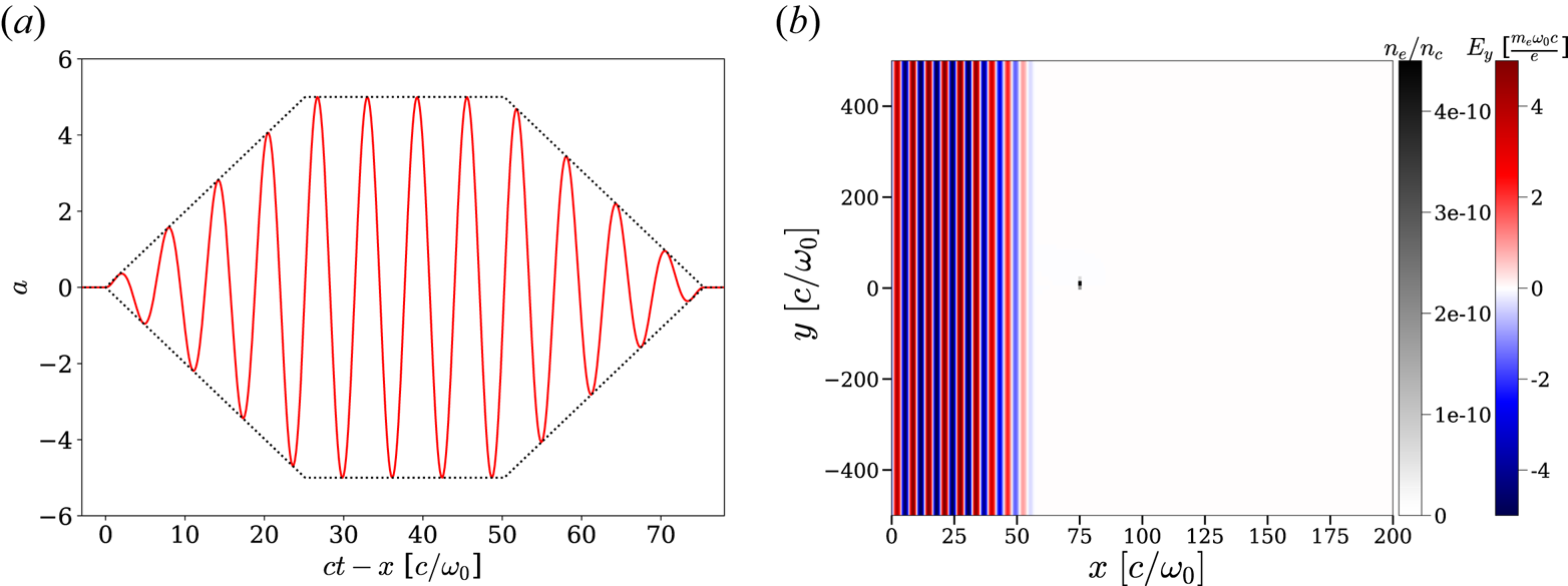
The propagating wave's temporal profile has a finite extension with a trapezoidal envelope as shown in figure 3(a). Each ramp and the plateau of the trapezoidal profile are $4 \lambda _0$ long. We take care that $\int E_y(t)\,{\rm d}t = 0$
 , otherwise $A_y$
 , and thus $p_y$
 , is non-zero even once the laser has passed. To make the analysis easier we also chose the temporal profile so that $\int _{t_1}^{t_2} E_y(t) \,{\rm d}t = 0$
 , with $t_1$
 and $t_2$
 being the time boundaries of the profile ramps or plateau. This ensures that the transverse impulsion $p_y$
 is zero on average during the whole passing of the laser intensity plateau by the electron.
(a) Temporal profile (normalised vector potential $a$ ) of the incident wave. The dashed line describes the trapezoidal envelope. (b) Initial situation of the simulation. The incident wave is propagating to the right.

Only one particle is considered here. It is initially at rest at the centre of the simulation box. This single particle is given a very small statistical weight in the simulation so that the charge density (computed within each cell of the simulation) around the particle is negligible and does not affect the particle dynamic. Figure 3(b) shows the initial state of the simulation. It is an electron density map (normalised to the plasma critical density $n_c = \epsilon _0 m_e \omega _0^2 / e^2$ ) showing the initial position of the particle superimposed on a map of the wave transverse electric field $E_y$
 .
Considering a propagating plane wave along $x$ , polarised along the $y$
 axis and with a temporal envelope $f$
 such as $\boldsymbol {A} = A_0 f(t - x/c) \sin (\omega _0 (t - x/c) ) \boldsymbol {e_y}$
 , then (2.5), (2.6) and (2.7) may be rewritten as


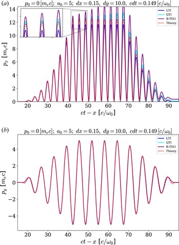
Figure 4 shows results for each simulation by comparing the particle momenta $p_x$ and $p_y$
 with those expected according to theoretical computations based on (2.12) and (2.13). These figures use normalised values, meaning $t$
 is expressed as multiples of $1/\omega _0$
 , $x$
 as multiples of $c/\omega _0$
 and the momentum $p$
 as multiples of $m_e c$
 .


The QTI and B-TIS methods give values of $p_y$ closer to the theoretical value than LTI but, overall, all three simulations reproduce fairly well the transverse behaviour of the particle with small differences.
Still, notable differences between analytical and simulation results though are present at the beginning and end of the trapezoid ramps ($t-x \approx 20$ and $t-x \approx 90$
 ) in figure 4(b). Those are due to a small difference in how the laser temporal profile is defined: in the theoretical case we considered a trapezoidal envelope for the vector potential $A$
 , whereas we considered a trapezoidal envelope for the electric and magnetic fields $E$
 and $B$
 in the simulation, as it is easier to initialise the value of those fields. This definition gives rise to vector potential $A$
 with a slightly different shape when $A$
 varies significantly within a single wavelength, as is the case at the boundaries of the temporal profile of the wave.
The longitudinal momentum is more problematic and only the LTI method reproduces qualitatively the expected behaviour of the particle, with a notable error on the maximal value of $p_x$ which is underestimated. Both QTI and B-TIS lead to an overestimation of $p_x$
 with an error increasing over time (artificial increase in the energy of the particle). This error leads to a non-physical residual momentum after the wave has gone by.
In the next section we investigate the source of this error and present a possible solution for the B-TIS method.
2.3. Inaccurate longitudinal momentum with QTI and B-TIS
The laser wave propagation in Calder is computed using the fields $E$ and $B$
 not the vector potential $A$
 so we will use here expressions with respect to the electromagnetic fields. The electron motion equation, for the longitudinal momentum, is thus

Considering a plane wave propagating along $x$ and polarised along the $y$
 axis such that $E_y = E_0 \cos ( \varphi )$
 with $\varphi = \omega _0 (t-x/c)$
 , then $B_z = (E_0 / c) \cos ( \varphi )$
 and $E_x = 0$
 , $B_y =0$
 . The previous equation thus becomes

From (2.6), we get that $v_y \propto A(\varphi ) \propto \sin ( \varphi )$ , which leads to

This means that for an electron initially at rest, after an integer number of wave periods, the momentum $p_x$ should be $0$
 again as $\int _0^{2{\rm \pi} } \sin ( \varphi ) \cos ( \varphi ) \,{\rm d}\varphi = 0$
 . This is indeed what is observed in figure 4 for the theoretical curve and LTI but not for QTI and B-TIS. This error comes from the computational error introduced during the magnetic field interpolation step.
Looking at (2.9)–(2.11), for all three methods, we can see that the error depends on a term that is proportional to $\cos (\varphi )$ but in the case of QTI and B-TIS there is a second term proportional to $\sin (\varphi )$
 . It is this last part which is problematic here. Taking a look at the numerically computed momentum $p_x^{{\rm num}}$
 in our simulation, we can express it as

where $\varepsilon _p$ is the numerical error on the momentum $p_x$
 . Thus, with LTI, we get that

with $K$ a constant depending on the wave amplitude. This error will fluctuate with time but it will periodically cancel out, whereas with QTI and B-TIS we get


with $K' = K ( 1 - \cos ( \delta \varphi ) ( 1 + \tfrac {1}{2} \sin ^2 ( \delta \varphi ) ) )$ and $K'' = K ( 1 - \cos ( \widehat {\delta \varphi } ) )$
 . The second term in these expressions leads to an error that grows continuously and monotonically with time instead of periodically cancelling out. This explains the divergence of results observed in figure 4 though the initial error is really small. Note also that, with our values for the parameters $\Delta x$
 and $\Delta t$
 , $\tfrac {1}{2} \sin ^3 ( \delta \varphi ) \approx 2\times 10^{-4}$
 whereas $\sin ( \widehat {\delta \varphi } ) \approx 5\times 10^{-4}$
 . This explains the difference in growth rate for the error with QTI and B-TIS.
The obvious solution would be to use a finer grid so as to minimise $\Delta t$ and $\Delta x - c \Delta t$
 – thus minimising $\delta \varphi$
 , $\widehat {\delta \varphi }$
 and the induced error – but this is highly detrimental to computation performance. Restricting oneself to using only small values of $a_0$
 is another way to circumvent this problem – as the error is proportional to $a_0^2$
 – but it is problematic in the case of the study of VLA or DLA. In any case, both of those approaches only mitigate the problem as the error will still be present and, though small initially, it will compound and increase with time.
It is, however, possible to slightly modify B-TIS in a way that drastically reduces this source of error while still benefiting from all of the advantages of this method.
2.4. B-TIS modification
As we saw earlier, B-TIS replaces the following temporal interpolation of the magnetic field:

with the following translation (as shown in figure 2a):

This is based on the assumption that the wave propagates at $c$ along the $x$
 axis and that $c \Delta t \approx \Delta x$
 .
However, if the value of the magnetic field is conserved going forward in time and space, it is also conserved when going backward, and within those assumptions, that translation is completely equivalent to

Both possible translations are shown in figure 2(b) where the assumption that the magnetic field $B$ propagates at $c$
 and that $c \Delta t \approx \Delta x$
 means that $B$
 is constant along the diagonals of the grid, hence the equivalence of the two translations.
Let us call rB-TIS the ‘reversed’ version of B-TIS using $\hat {B}_i^n = B_{i-{1}/{2}}^{n-{1}/{2}}$ . This method then introduces the following error on the magnetic field:


With the exception of the sign of the second term, this is the same expression as the error for the ‘classical’ B-TIS. As such, we should be able to eliminate that second term by combining both B-TIS and rB-TIS. We can indeed choose to use both translations in conjunction at each time step through a simple average such as

It is important to note, though, that it is not a simple temporal averaging as is used in LTI: both the time index and the spatial index are different. This new method, which we call B-TIS3, then introduces the following error on $B$ :


The second term involving $\sin (\varphi )$ has indeed disappeared as we expected. The expression of this error is similar to the one introduced by LTI with the important difference though that we have $\widehat {\delta \varphi } < \delta \varphi$
 , which should point to an improvement of accuracy.
To illustrate this point, let us consider a forward-propagating wave in a vacuum with $\omega = \omega _0$ and $k_x = k = {\omega _0}/{c}$
 . We thus have $\delta \varphi = {\omega _0 \Delta t}/{2}$
 while $\widehat {\delta \varphi } = \tfrac {1}{2} ({\omega _0}/{c}) ( \Delta x - c \Delta t )$
 .
Then, per (2.9), (2.10), (2.11) and (2.29), with our numerical parameters we get


On the other hand, let us consider a wave, propagating forward in the simulation at the Nyquist frequency so that $\omega = {{\rm \pi} }/{\Delta t}$ and $k_x = k = {{\rm \pi} }/{\Delta x}$
 . Then, as $\delta \varphi = {{\rm \pi} }/{2}$
 and $\widehat {\delta \varphi } = 0$
 :


Both of these simple cases show the immense improvement in accuracy that B-TIS3 brings to our simulations regarding the magnetic field over all the previously considered methods.
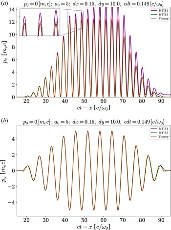
A comparison of the results from the B-TIS3 method and the previous one is presented in figure 5. We can see that this improved B-TIS3 eliminates the troublesome compounding error impacting B-TIS1 and leads to computed values of $p_x$ even closer to the theoretical ones than those obtained using LTI. Results on transverse momentum $p_y$
 are just as good as before, the improvement margin being already very slim even with LTI.


At this point, the reader should note that we have focused on forward-propagating waves, as they are those that are most commonly encountered in VLA and LWFA and for which this scheme was designed. Counter-propagating radiation, however, can be present in a few situations, because of backscattering for instance or even in the case of colliding laser pulses. It is thus of interest to check the robustness of our new scheme in such scenarios.
The accuracy of both LTI and QTI is not impacted for a counter-propagating wave, as we still have $\delta \varphi = {\omega \Delta t}/{2}$ . For B-TIS and B-TIS3, however, with $k_x = -k$
 , we now get $\widehat {\delta \varphi } = ( k \Delta x + \omega \Delta t )/2$
 . With this, for a counter-propagating laser pulse we get

And for a wave propagating backward at the Nyquist frequency:

While these results appear much worse than in the case of forward propagation, it should be noted that they are not that different from the accuracy level of LTI, with a factor of 2 to 4 between them. Therefore, the presence of counter-propagating radiation in the simulation, although not the ideal use case for B-TIS3, should not prove physics-breaking and the overall gains might be well worth this trade-off.
From these results, it appears that we have successfully solved the initial problem encountered in the computation of the longitudinal momentum $p_x$ and that B-TIS3 appears well suited to reproduce the physics of VLA contrary to B-TIS1 and QTI.
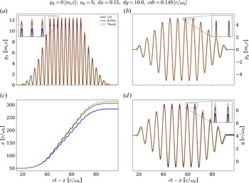
As LTI is by far the most common method used in PIC codes, it seems an appropriate method with which to compare. We then only present simulation results for both of these methods. A summary of results for LTI and B-TIS3 is presented in figure 6. The better reproduction of the momentum with B-TIS3 shown in figure 6(a,b) leads to an electron trajectory more faithful to the theoretical predictions as can be seen in figure 6(c,d).
Evolution of the electron normalised momentum (a) $p_x$ and (b) $p_y$
 and normalised position (c) $x$
 and (d) $y$
 with respect to the normalised coordinate $ct-x$
 for LTI and B-TIS3. The red dashed line shows the theoretical values expected from the analytical model introduced earlier.

2.5. Simulations with initial longitudinal momentum
We have so far investigated only the case of an electron initially at rest but, in practice, electrons are far more likely to have a non-zero initial momentum. Going back to the analytical model developed in § 2.1, with $p_{x,0} \neq 0$ and $\gamma _0 \neq 1$
 we now get

which leads to the three following equations now describing the electron motion:


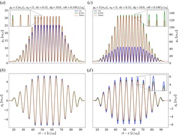
Figure 7 shows results from two simulations where the electron had an initial longitudinal momentum $p_0$ : the first one with $p_0 = m_e c$
 and the second one with $p_0 = 5 m_e c$
 . All other numerical and physical parameters are the same as previously. The two methods result in much more noticeable differences than previously.
Evolution of the electron normalised momentum (a) (respectively c) $p_x$ and (b) (respectively d) $p_y$
 with respect to the normalised coordinate $ct-x$
 for LTI and B-TIS3 with $p_0 = m_e\, c$
 (respectively $p_0 = 5\, m_e\, c$
 ). The red dashed line shows the theoretical values expected from the analytical model introduced earlier.

It is apparent that the greater the initial velocity of the electron, the more LTI underestimates the longitudinal momentum. The maximum longitudinal momentum $p_{x,max}$ being underestimated by a factor of at least $3$
 compared with the theoretical value when using LTI with an initial momentum $p_0 = 5\, m_e\, c$
 . B-TIS3, on the other hand, slightly overestimates $p_x$
 but overall produces results much closer to the predictions of the analytical model.
Looking now at the transverse momentum $p_y$ , both methods reproduce fairly well the theoretical results, though both tend to overestimate them. Once again, the B-TIS3 results appear closer to those of the model and, though the error increases when the initial momentum $p_0$
 increases, this increase appears much smaller for B-TIS3 than for LTI.
Note that all of the presented simulations have been realised using the Boris pusher (Boris Reference Boris1970). We found very negligible differences between simulations using the Boris scheme and simulations using the scheme proposed in Vay (Reference Vay2008) to correct the Boris pusher inaccuracies at relativistic speed, and we observed the same inaccuracies with LTI and the same improvements with B-TIS3, irrespective of the choice of pusher.
3. Interaction with a Gaussian beam
In order to get to more realistic cases, we now consider, as our incident wave, a laser pulse with a Gaussian spatial profile instead of plane wave with an infinite transverse size.
3.1. Theoretical description
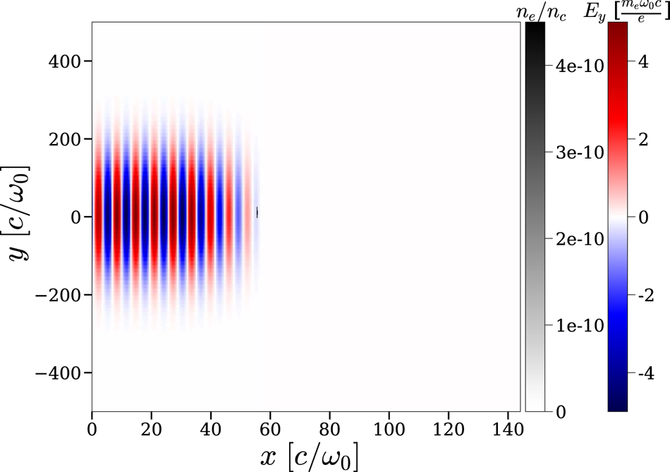
We keep the same trapezoidal temporal profile for our laser pulse so as to make comparisons with earlier results easier; however, its transverse size is now finite and given by a Gaussian profile with a width (full width at half maximum of the intensity profile) of $160 \omega _0/c$ . Figure 8 shows this initial situation.
Initial situation with a spatially Gaussian wave.

We can come back to the equations introduced in § 2.1 but considering now the more general case of a wave polarised along the $y$ axis and propagating along the $x$
 axis such that $\boldsymbol {A}(x,y,t) = A(x,y,t) \boldsymbol {e}_y$
 . The laser waist is assumed here much larger than the wavelength and as such we can neglect the existence of a vector potential component along $x$
 (we discuss this approximation later). The energy conservation equation then leads to

And the motion equation (2.1) gives us


Using the fact that ${{\rm d} \boldsymbol {A}}/{{\rm d}t} = {\partial \boldsymbol {A}}/{\partial t} + ( \boldsymbol {v} \boldsymbol {\cdot } \boldsymbol {\nabla } ) \boldsymbol {A}$ , we finally get to


This system is much more complex than the previous one and we do not attempt to solve it analytically here. We can still gather though that the ponderomotive force of the laser will push aside the electron and that it will gain a residual momentum, both longitudinal and transverse. For an exact solution of the motion and acceleration of electrons by the laser fields, we would have to consider the longitudinal component of $\boldsymbol {A}$ ($\boldsymbol {A}=A_x\boldsymbol {e_x}+A_y\boldsymbol {e_y}$
 ) which would modify (3.1) from (3.6) above. For simplicity's sake, however, we do not consider the component $A_x$
 which is negligible in our case. More comprehensive descriptions and computations on this subject can be found in Mora & Antonsen (Reference Mora and Antonsen1997) and Quesnel & Mora (Reference Quesnel and Mora1998).
3.2. Numerical results
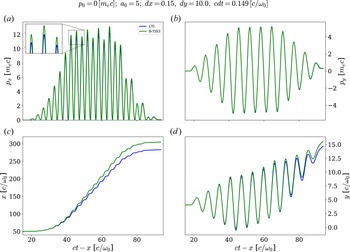
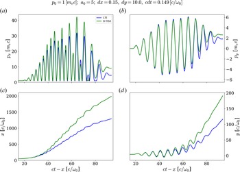
Figures 9 and 10 sum up the simulation results for an electron initially close to the propagation axis and, respectively, with no initial longitudinal momentum ($p_0 = 0$ ) or with $p_0 = m_e c$
 .
Evolution of the electron normalised momentum (a) $p_x$ and (b) $p_y$
 and normalised position (c) $x$
 and (d) $y$
 with respect to the normalised coordinate $ct-x$
 for LTI and B-TIS3 with a transversely Gaussian laser beam and an electron initially at rest ($p_0 = 0$
 ).

Evolution of the electron normalised momentum (a) $p_x$ and (b) $p_y$
 and normalised position (c) $x$
 and (d) $y$
 with respect to the normalised coordinate $ct-x$
 for LTI and B-TIS3 with a transversely Gaussian laser beam and an electron with an initial longitudinal momentum ($p_0 = m_e c$
 ).

The behaviour observed in the simulations is in accordance with our expectations: the electron drifts transversely as it is being accelerated and thus ends up with residual non-zero longitudinal and transverse momentum, $p_x$ and $p_y$
 , even after it has exited the laser beam. This residual extra momentum is quite small when the electron is initially at rest but it quickly becomes more important when the electron has some initial velocity as we can see in figure 10(a,b).
Both methods predict overall a similar behaviour for the electron though we can observe notable differences in final momentum and positions. Indeed as the electron is evidently more accelerated in the B-TIS3 case, it travels a much longer distance while inside the laser pulse. This difference is especially apparent in the case with a non-zero initial momentum, which is coherent with our previous observations.
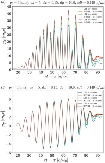
As we cannot compare with an analytical model here, we use a numerical method to estimate the theoretical result. When reducing both the spatial grid size and the time step duration, both numerical methods should converge on a unique solution corresponding to the physical solution.
We look at the results of three pairs of simulations where we chose $\Delta x = 0.15 c/\omega _0$ and $c \Delta t = 0.149 c/\omega _0$
 for the first one, $\Delta x = 0.10 c/\omega _0$
 and $c \Delta t = 0.099 c/\omega _0$
 for the second and $\Delta x = 0.05 c/\omega _0$
 and $c \Delta t = 0.049 c/\omega _0$
 for the third. Observed momenta are shown in figure 11. Those results clearly show that both methods are converging on the same solution which appears fairly close to the one obtained initially through B-TIS3. We thus observe once again that B-TIS3 tends to slightly overestimate the electron momentum while LTI noticeably underestimates it.
Evolution of the electron normalised momentum (a) $p_x$ and (b) $p_y$
 with respect to the normalised coordinate $ct-x$
 for LTI and B-TIS3, with $p_0 = \, m_e c$
 and varying cell sizes and time steps.

It is important to note, however, that even when dividing by 3 both $\Delta t$ and $\Delta x$
 (thus increasing the computation time by a factor of 9), LTI still does not give better results than B-TIS3 with a worse resolution. B-TIS3 appears, in that light, as a fairly good improvement on the standard LTI.
3.3. Influence of the initial position
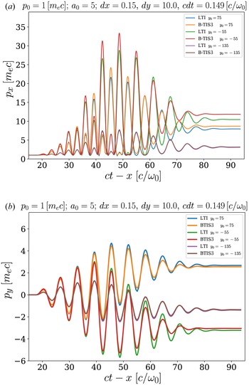
The ponderomotive force acting on a particle depends on the laser pulse intensity gradient which varies widely depending on the transverse position.
We show in this section that we can indeed observe this behaviour in our simulations. We present here in figure 12 the momenta of electrons with different initial positions $y_0$ .
Evolution of the electron normalised momentum (a) $p_x$ and (b) $p_y$
 with respect to the normalised coordinate $ct-x$
 for LTI and B-TIS3, with $p_0 = \, m_e c$
 and varying initial transverse position $y_0$
 of the electron. Note that the transverse profile of the laser is centred on $y=0$
 .

Both methods tend to predict similar final momentum for the electron as long as it is outside of the stronger field region of the laser pulse. Indeed differences in results between LTI and B-TIS3 are less important the farther is the electron initially from the propagation axis.
As we showed that the error introduced by LTI was greater when the electron was strongly accelerated, it thus seems logical that its predictions are better – thus more in accordance with B-TIS3 – when the electron is far from the high-intensity region near the propagation axis and less accelerated.
Though final momentum may appear similar, the small differences can have a great impact on the particle trajectory. Furthermore, when trying to study VLA we are of course more interested in the strongly accelerated electrons. Thus the usage of the B-TIS3 method appears better suited to these simulations than the standard LTI.
4. Results for VLA and DLA simulations
4.1. Vacuum laser acceleration simulations
Now that we have determined that B-TIS3 gives more accurate results than LTI for a single electron, we want to simulate a bunch of electrons and see the impact of the different methods on more realistic cases. We thus introduce in our simulation a full electron beam instead of a single particle while keeping the same laser profiles as described in § 3. The initial situation is presented in figure 13. Note that we chose here to initialise the electron beam directly in the laser field so as to maximise electron acceleration. The (two-dimensional) charge of the beam is quite low (${\approx }4.5\, {\rm pC}\,\mathrm {\mu }{\rm m}^{-1}$ ) so as to limit space charge effects and both the longitudinal and transverse spatial extensions are chosen to be close to a laser wavelength of $800 \,{\rm nm}$
 .
Initial situation with a spatially Gaussian laser beam and an electron bunch.

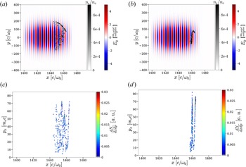
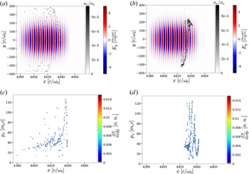
Still comparing results of simulations using either LTI or B-TIS3, in both simulations we observe the electron beam being longitudinally accelerated with the laser ponderomotive force making it gradually blow up. The electrons then exit the laser pulse, mostly through the sides without making it through longitudinally from end to end. Electrons are, however, accelerated for much longer in the B-TIS3 simulation, resulting in the charge being contained in the simulation box for a much longer propagation distance, as we can see in figure 14.
Charge inside the simulation box with respect to travelled length.

Figures 15 and 16 give a comparison of the spatial positions of the electrons within the laser beam as well as their phase space $(x,p_x)$ for two different times of the simulation. As expected, we can see that the beam is progressively bursting apart due to the laser ponderomotive force. The asymmetry in the explosion of the beam is due to the fact that the electron bunch is initially not exactly on the propagation axis but in fact slightly above it, hence the drift mostly towards positive values of $y$
 . Also, as the electron beam is initially about as long as a laser wavelength, the back-end and the front-end are not in phase. They interact initially with fields of different values – thus feel different forces which explains the progressive separation of the two ends of the beam.
Electronic density map (greyscale) superimposed to the electric field $E_y$ map (colours) after a propagation of $570\,\mathrm {\mu }{\rm m}$
 for (a) LTI and (b) B-TIS3. Phase space $(x,p_x)$
 after a propagation of $570\,\mathrm {\mu }{\rm m}$
 for (c) LTI and (d) B-TIS3.

Electronic density map (greyscale) superimposed to the electric field $E_y$ map (colours) after a propagation of $950\,\mathrm {\mu }{\rm m}$
 for (a) LTI and (b) B-TIS3. Phase space $(x,p_x)$
 after a propagation of $950\,\mathrm {\mu }{\rm m}$
 for (c) LTI and (d) B-TIS3.

We can see in figure 15(a,b) that the beam is dispersed much more quickly in the simulation using LTI compared to that using B-TIS3, and it is even more apparent in figure 16(a) where there is almost no electron left in the laser beam while the electron bunch is, at the same time, still clearly present in figure 16(b) for B-TIS3. The periodic evolution of $p_x$ that we saw earlier is also visible on the map of the $(x,p_x)$
 phase space, especially in figures 15(d) and 16(d). Though this structure is quickly masked in the case of LTI, we can still make it out in figure 15(c).
Figure 17 shows a comparison of the electron energy spectra after two different propagation lengths. The remaining charge inside the simulation window is much more important in the case of B-TIS3 and reaches higher energies which is coherent with previous observations.
Energy spectrum of the accelerated electrons after a propagation of (a) $570\,\mathrm {\mu }{\rm m}$ and (b) $950\,\mathrm {\mu }{\rm m}$
 .

In the end, it appears that B-TIS3 produces results significantly different from those of LTI. Considering those results and the previous comparison with theoretical models, LTI appears – barring a prohibitively costly refining of the grid – to not be well suited to the study of VLA though B-TIS3 may be an easy-to-implement substitute to solve this problem. Indeed, LTI may lead to an inadequate estimation of the accelerated charge and of the beam energy, two key characteristics in electron acceleration.
4.2. Direct laser acceleration simulations
Investigating the use of B-TIS3 for VLA simulation has allowed us to highlight its improvement compared with LTI. However, as VLA so far has been shown to be quite limited as a reliable source of accelerated electrons, it is interesting to also study the use of B-TIS3 in simulations of other acceleration methods.
We already demonstrated the usefulness of B-TIS in mitigating the impact of numerical artefacts such as NCR in LWFA simulations (Bourgeois & Davoine Reference Bourgeois and Davoine2020) and those results still apply with B-TIS3. In addition to this, our new interpolation technique, B-TIS3, should also bring great improvements to simulations of another situation: DLA.
In LWFA, DLA occurs when the laser beam is long enough to encompass part of the bubble where electrons are being accelerated which brings about a coupling between electrons and laser fields (Pukhov et al. Reference Pukhov, Sheng and ter Vehn1999). Those electrons are then subject not only to the electromagnetic wake fields but also to those of the laser pulse and their energy gain is, in part, due directly to the laser wave and not only to the plasma wave.
To investigate this setting, we performed two two-dimensional simulations (one using LTI the other B-TIS3), choosing laser and plasma parameters leading to the creation of a wakefield with efficient electron acceleration but with a purposefully elongated temporal profile for the laser, facilitating interaction between the accelerated electrons and the laser field so as to get DLA. Figure 18 shows the temporal profile of the laser used in the simulation which is realised by adding two Gaussian temporal profiles with different amplitudes, lengths and delays ($a_0 = 6$ , $\tau = 42\, {\rm fs}$
 for the first profile, where $\tau$
 is the laser intensity profile full width at half maximum, and $a_0 = 4$
 , $\tau = 85\, {\rm fs}$
 for the second one with a $42\, {\rm fs}$
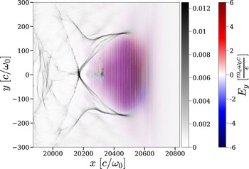
 delay between the two maximums). This results in an asymmetric temporal profile with duration of around 100 fs: the high-intensity pulse front generates the wakefield while the low-intensity pulse tail fills the back of the bubble and interact with the electron beam as shown in figure 19. This laser profile was specifically designed to favour laser interaction with an accelerated electron beam and DLA in a fast two-dimensional simulation.
Temporal profile of the electric field $E_y$ .

Electron density map normalised to the critical density $n_c$ (greyscale) superimposed to the electric field $E_y$
 map.

This laser is propagating in a 6 mm long and fully ionised plasma with an electron density of $n_e = 0.0025 n_c$ . We used a density gradient injection technique (Bulanov et al. Reference Bulanov, Naumova, Pegoraro and Sakai1998; Suk et al. Reference Suk, Barov, Rosenzweig and Esarey2001; Ekerfelt et al. Reference Ekerfelt, Hansson, Gallardo González, Davoine and Lundh2017) to facilitate electron injection in the bubble. The simulation is performed inside a moving window of $6400 \times 400$
 cells with $c \Delta t = 0.149 c/\omega _0$
 , $\Delta x = 0.15 c/\omega _0$
 and $\Delta y = 3 c/\omega _0$
 .
Figure 19 gives an example of DLA in a numerical simulation. As in all LWFA cases, the laser propagating inside the plasma excites a plasma wave in its wake which creates a positively charged cavity in which electrons can be accelerated. The borders of this cavity or bubble are delimited by a higher electron density and easily visible on the greyscale map. A beam of electrons has already been injected and is being accelerated inside of the bubble around $y=0 c/\omega _0$ and $x=20\,350 c/\omega _0$
 . The laser oscillations are easily visible and present over the whole length of the bubble meaning all of the injected electrons are directly influenced by the laser field.
Both simulations predict the formation of an accelerating bubble in the wake of the laser beam and the injection and subsequent acceleration of a similar charge of electrons. Note that contrary to what was done in our previous paper (Bourgeois & Davoine Reference Bourgeois and Davoine2020), B-TIS3 is now applied to all electrons in the simulation, irrespective of their energy.
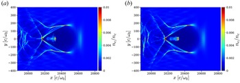
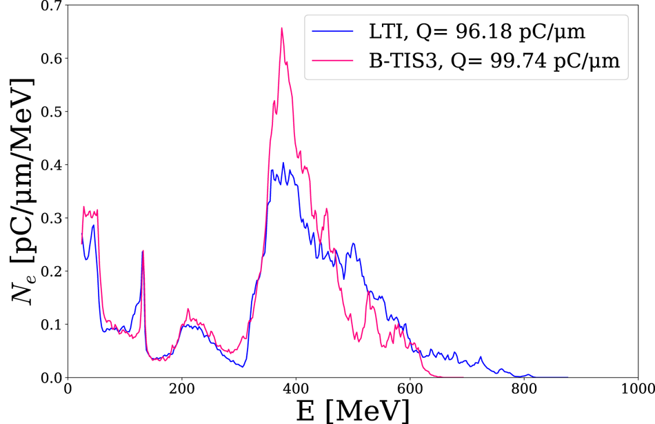
There are nevertheless significant differences between the two simulations. The electron beam appears much more focused in the B-TIS3 case. This effect is visible directly on the transverse size of the beam as can be seen in figure 20, but also on the transverse momentum of the accelerated electrons as shown in figure 21. It is important to note that NCR is quite weak in these two-dimensional simulations and thus this numerical artefact is not responsible for this variation in beam transverse size and divergence in the way we observed in Bourgeois & Davoine (Reference Bourgeois and Davoine2020). In the present case, the difference is indeed due to the improved modellisation of the laser–electron interaction in the B-TIS3 simulation. Comparing the electron phase space $(p_x,\, p_y)$ of both simulations, we can see that both beams have a similar structure but with a much higher dispersion in the LTI case, especially for the transverse momentum of the most energetic electrons. This seems to be in accordance with previous observations suggesting LTI tends to overestimate $p_y$
 and thus the beam divergence. However, somewhat contrary to what could be expected, LTI also predicts higher longitudinal momentum than B-TIS3 despite the fact that we showed in our previous VLA simulations that LTI tends to underestimate $p_x$
 when B-TIS3 slightly overestimates it. This difference may be explained by the fact that electrons are not accelerated only by laser fields as was previously the case. Direct laser acceleration is the result of a complex coupling between the laser and the plasma fields and a small error on the laser field effect can lead to an important perturbation of this coupling, leading to the overestimation of both $p_y$
 and $p_x$
 .
Electron density map after 2.65 mm of laser propagation in the plasma: (a) LTI simulation; (b) B-TIS3 simulation.

Phase space map $(p_x,\, p_y)$ after 2.65 mm of laser propagation in the plasma: (a) LTI simulation; (b) B-TIS3 simulation.

Looking at the energy spectra of both beams (figure 22), we can again observe the previously noted similarities and differences: LTI presents a broader spectrum which reaches to higher energies whereas the B-TIS3 spectrum is much more peaked.
Energy spectrum of the accelerated electrons after 2.65 mm of laser propagation in the plasma.

The overall similarity of those two simulations leads us to think that B-TIS3 does not introduce adverse effects to the modellisation of DLA in our simulation. To the contrary in fact, the previous results for the VLA simulations make us confident in the fact that the modellisation of laser–electron interaction is improved by the use of B-TIS3 over LTI leading to a better reproduction of the electron behaviour in both VLA and DLA.
Note that DLA simulations presented here had relatively low electronic densities. Simulations with higher densities were also performed and we found that differences between simulations using LTI or B-TIS3 are less and less prevalent with higher electronic densities ($n_e \approx 0.01 n_c$ or higher) to the point of becoming almost negligible. We can assume that, in those regimes, the plasma impacts the laser propagation sufficiently so that there are real, physical differences in amplitude between the electric and magnetic fields of the laser, making the error on the $B$
 amplitude introduced by LTI negligible.
5. Conclusion
In this paper we improved upon the already introduced technique of B-TIS, making it more robust and accurate. We then demonstrated its usefulness, not only to mitigate adverse effects of NCR, but also to better model laser–electron interaction phenomena, getting more faithful results, especially in terms of momentum, than the traditional PIC methods. These improvements appear particularly important in the case of VLA simulations or simulations involving DLA with low electron densities where those small differences lead to more realistic values of charge and energy for the accelerated electron beams.
With the benefit of this technique established, it could now be used to study more complex cases of LWFA, DLA, VLA or other situations where electron beam or plasma co-propagates with an electromagnetic pulse in a PIC simulation box. For instance, VLA with a radially polarised laser (Zaïm et al. Reference Zaïm, Thévenet, Lifschitz and Faure2017) could benefit from this improved modellisation to better understand the polarisation impact and effects of other properties on the acceleration process.
Acknowledgements
Editor L.O. Silva thanks the referees for their advice in evaluating this article.
Funding
This work has been supported by Laserlab-Europe (EU-H2020 654148). We also acknowledge GENCI for granting us access to the supercomputer Irene under grant nos. A0110512993 and A0100507594.
Declaration of interests
The authors report no conflict of interest.