1. Introduction
Passive micromixers were one of the first element to be added to the microfluidic toolbox. Early systems, such as T-mixers (Kamholz et al. Reference Kamholz, Weigl, Finlayson and Yager1999), H-filters (Brody & Yager Reference Brody and Yager1997) and hydrodynamic focusing chips (Knight et al. Reference Knight, Vishwanath, Brody and Austin1998), were used for the design of separation systems (Weigl & Yager Reference Weigl and Yager1999), diffusion-based assays (Hatch et al. Reference Hatch, Kamholz, Hawkins, Munson, Schilling, Weigl and Yager2001) and controlled chemistry at interfaces (Atencia & Beebe Reference Atencia and Beebe2005). These systems usually operate at high Péclet numbers and exchange between the different incoming streams happens by slow, linear diffusion. As rapid mixing equipment, these simpler systems were eventually replaced by chaotic mixers (Stroock et al. Reference Stroock, Dertinger, Ajdari, Mezic, Stone and Whitesides2002), which use ‘stretch-and-fold’ dynamics to enact mixing in time scales orders of magnitude more rapid than passive diffusion (Ottino & Wiggins Reference Ottino and Wiggins2004).
In recent years, however, there has been a renewal of interest for more complex system geometries that still exhibit passive advection–diffusion, free of chaotic features. In pharmaceutical applications, devices based on variants of hydrodynamic focusing chips have been used as tools for the synthesis of complex lipid particles, first liposomes (Jahn et al. Reference Jahn, Vreeland, DeVoe, Locascio and Gaitan2007; van Swaay & DeMello Reference van Swaay and deMello2013), then lipid nanoparticles (Krzysztoń et al. Reference Krzysztoń, Salem, Lee, Schwake, Wagner and Rädler2017). The synthesis of these particles is typically done using rapid solvent–antisolvent mixing, where an organic stream containing precursor lipids is rapidly mixed with an aqueous stream containing payload molecules (Buschmann et al. Reference Buschmann, Carrasco, Alishetty, Paige, Alameh and Weissman2021). A current active area of research in the field is the precise determination of process-property parameters (Devos et al. Reference Devos2024) and the mixing equipment is known to have an important impact on final product characteristics, as shown by the few systematic studies investigating similar formulations with different mixers (O’Brien Laramy et al. Reference Laramy2023; Petersen et al. Reference Petersen, Chaudhary, Arral, Weiss and Whitehead2023; Chen et al. Reference Chen, Liu, Guo, Yang, Zhao and Yang2025). Formation of liposomes and other small lipid vesicles is known to be a kinetic, non-equilibrium process (Leng, Egelhaaf & Cates Reference Leng, Egelhaaf and Cates2003). As such, simple equilibrium considerations (Lasic et al. Reference Lasic, Joannic, Keller, Frederik and Auvray2001) are inadequate in predicting output, and a detailed knowledge of the microenvironment history of individual lipid nanoparticles during their formation is necessary for a correct prediction of their final morphology. Microfluidic mixers offer a unique opportunity to probe these complex self-assembly mechanisms. Flow and concentration gradients within them are much more regular and predictable than in their chaotic or turbulent counterparts. This makes the precise determination of the flow and concentration everywhere within them feasible. This regularity allows for the probing of the microenvironment of nucleating particles with a granularity that is impossible in larger mixers. Low-enough-Reynolds-number mixers have the advantage of being amenable to analytic treatment, which can considerably speed up calculations and give insight into scaling behaviour that would otherwise be laborious to obtain from numerical studies. There is a clear need for precise analytical models of transport in these microfluidic mixers. Such models should give us complete information about flow and diffusion in experiments, such as the solvent–antisolvent precipitation used in nanoparticle formation, and be applicable to the wide range of mixer geometry that currently exists.
Problems of complex planar flow have a long history of analytical treatment. Potential flow theory, combined with complex variable methods, has been a mainstay of theoretical hydrodynamics, from the pioneering work of Lamb (Reference Lamb1924) and Milne-Thomson (Reference Milne-Thomson1943), to its application to planar Darcy flows, omnipresent in groundwater mechanics (Strack Reference Strack1988). Methods based on conformal transforms have also been used to study other transport problems associated with these flows. Starting with Boussinesq (Reference Boussinesq1902), it has been known that advection–diffusion in planar potential flow is conformally invariant. Similar transformations to that used by Boussinesq were later applied to the study of turbulent dispersion of pollution by wind (Hunt Reference Hunt1973; Hunt & Mulhearn Reference Hunt and Mulhearn1973), to tracer dispersion in porous media (Koplik, Redner & Hinch Reference Koplik, Redner and Hinch1994), to solidification problems (Cummings et al. Reference Cummings, Hohlov, Howison and Kornev1999) and to dispersion by bluff bodies (Eames & Bush Reference Eames and Bush1999), just to name a few. Work by Martin Bazant in the 2000s showed how the Boussinesq problem was a specific example of a wider family of conformally invariant systems (Bazant Reference Bazant2004) and later applied the method to problems of non-Laplacian growth (Choi et al. Reference Choi, Margetis, Squires and Bazant2005), as well as the elaboration of three-dimensional (3-D) solutions of the Navier–Stokes equation (Bazant & Moffatt Reference Bazant and Moffatt2005). The same methodology was used to study induced recirculation in problems of magnetohydrodynamics in the Hele-Shaw cell (McKee Reference McKee2024). More recently, conformal mapping techniques have been applied to the determination of a steady-state concentration profile in a range of planar microfluidic systems. Arrangement of point sources and sinks have been used to study complex staining over surfaces (Goyette et al. Reference Goyette, Boulais, Normandeau, Laberge, Juncker and Gervais2019) and were subsequently shown to apply to large families of microfluidic systems (Boulais & Gervais Reference Boulais and Gervais2023). Similar flow and concentration patterns were simultaneously found to appear in the human choriocapillaris (Zouache, Eames & Luthert Reference Zouache, Eames and Luthert2015). Diffusion in channel junctions, such as T-sensors and hydrodynamic focusing chips, was studied using a combination of simplified semi-infinite channel geometry, and careful arrangements of point sources and sinks (Boulais & Gervais Reference Boulais and Gervais2020).
In this article, we extend this previously published body of work and present a theoretical framework for analysis of flow and diffusion in arbitrarily shaped microfluidic mixers. While previously cited work has focused on simple geometries (either radially symmetrical or based on simple rectangular channels), the method proposed here is applicable to mixers and channel junctions of arbitrary polygonal shapes, which is more representative of real mixing equipment. The method yields the exact concentration everywhere in the mixer, allowing for precise determination of the microenvironment history of individual particles, a crucial missing ingredient in the search for better models of self-assembly of lipid nanoparticles. The method presented here is based on the use of Schwarz–Christoffel maps (Driscoll Reference Driscoll2002), which have been known in the applied mathematics community for a long time, but have found very little applications in microfluidics and in pharmaceutical applications. Schwarz–Christoffel maps enabled the resolution of flow problems in complex channels (Floryan Reference Floryan1985), of general free surface flow problems (Dias, Elcrat & Trefethen Reference Dias, Elcrat and Trefethen1987) as well as problems of flow in porous media (Smith Reference Smith1996), but have been comparatively much less used in analysing the associated advection–diffusion problem that comes with these flows.
Using a sequence of conformal maps, we reduce the problem of advection–diffusion in a polygonal mixer to a known geometry and formulate an analytical solution for the velocity as well as the concentration profile everywhere in the mixer. One crucial map in the sequence, the map from an arbitrary polygon, has a set of unknown real parameters that need to be computed numerically. The method is thus semi-analytical. Since the map to and from the polygonal geometry only has to be computed once (as the mixer geometry does not change from one experiment to the next), the method allows for near instant determination of the concentration field and velocity, which could enable its use in control applications, where execution speed is often crucial. We focus here on microfluidic systems, given the comparatively more simple and regular characteristics of their flow and transport. Since flow in such systems can be kept laminar and free from chaotic features, they allow in principle a complete determination of flow and diffusion within them from knowledge about their input parameters (incoming flow rates, device dimensions, diffusion coefficients of components, etc.). However, the method of mapping shown here can also be used to generate grids that can serve as a starting point for efficient numerical analysis of more complex chaotic flows (Floryan Reference Floryan1985). Once we have outlined the models and shown how they can be used to analyse mixers of arbitrary geometries, we then move on to compare predicted results with experimental physical tracer tests.
2. Theory
2.1. Problem description
We are looking for a complete description of velocity and concentration profiles within a polygonal microfluidic mixer such as illustrated in figure 1. Such mixers typically have two or more inlets and a single outlet. In a typical flash nanoprecipitation experiment, the inlets will inject either solvent or antisolvent, the mixing of which we model using linear advection–diffusion. In some experiments, inlets may also have different initial temperatures, leading to temperature gradients on top of concentration gradients. As a first approximation, temperature gradients may also be modelled using linear advection–diffusion, but doing so neglects heat of mixing, which may become important in experiments involving the mixing of alcohol and water as solvent and antisolvent (Peeters & Huyskens Reference Peeters and Huyskens1993). Linear models may thus be applicable in cases where the difference in temperature between inlets is already much bigger than the difference in temperature generated by the heat of mixing. As a first approximation, we will suppose the Reynolds number to be low enough for creeping flow approximations to hold. This is adequate for typical hydrodynamic focusing systems (Knight et al. Reference Knight, Vishwanath, Brody and Austin1998; Jahn et al. Reference Jahn, Vreeland, DeVoe, Locascio and Gaitan2007), where rapid mixing is achieved by controlling the inlet ratio. This type of approximation breaks down for systems where inertial effects and chaotic mixing become important. We are focusing on quasi-planar geometries, where the mixer’s height is uniform and comparatively smaller than the other dimensions of the problem. This is consistent with standard methods of microfluidic system fabrication, and allows us to treat the problem as a quasi-two-dimensional (quasi-2-D) problem, which is common of many complex microfluidic flows (Boulais & Gervais Reference Boulais and Gervais2023).
Microfluidic mixer geometry. (a) Schematic of the mixer. (b) Experimental picture of a physical tracer test in a microfluidic impinging jet mixer (scale bar, 100
 $\mu$
m). (c) Different types of mixer geometries that have been published: (i) microfluidic analogue to an impinging jet mixer; (ii) Y-junction (Gobby, Angeli & Gavriilidis Reference Gobby, Angeli and Gavriilidis2001); (iii) hydrodynamic focusing system (Knight et al. Reference Knight, Vishwanath, Brody and Austin1998); (iv) multi-inlet hydrodynamic focusing (Park et al. Reference Park, Qiu, Rhoades, Korlach, Kwok, Zipfel, Webb and Pollack2006).

The method presented here allows for an arbitrary number of inlets and outlets, with each inlet fixed at a known concentration. Typical microfluidic mixers for nanoparticle synthesis may exhibit two (Hatch et al. Reference Hatch, Kamholz, Hawkins, Munson, Schilling, Weigl and Yager2001; Devos et al. Reference Devos2024), three (Knight et al. Reference Knight, Vishwanath, Brody and Austin1998) or a larger number of inlets (Park et al. Reference Park, Qiu, Rhoades, Korlach, Kwok, Zipfel, Webb and Pollack2006).
2.2. Constitutive equations
The equations describing the flow are the incompressible Navier–Stokes equation. If the depth of the mixer’s chamber is much smaller than the characteristic length in the horizontal direction, then the flow in the mixer can be adequately described as a Hele-Shaw cell. In that case, the Navier–Stokes equations reduce to the Hele-Shaw equations, which are easily solved for the in-plane velocity components (Batchelor Reference Batchelor2000),
 \begin{equation} u \approx - \frac {1}{2 \mu } \frac {\partial p}{\partial x} z ( d - z ), \hspace {3em} v \approx - \frac {1}{2 \mu } \frac {\partial p}{\partial y} z ( d - z ), \end{equation}
where
 $\mu$
is the viscosity of the fluid,
 $d$
the depth of the chamber and
 $p$
is the hydrostatic pressure. Equation (2.1) can be rewritten as
 \begin{equation} \boldsymbol{u} = - \boldsymbol{\nabla }\phi ( x, y ) z ( d - z ), \end{equation}
which is the product of a parabolic flow in the
 $z$
direction and the gradient of a 2-D potential function in the
 $xy$
plane. Combining (2.1) with the continuity equation
 $\boldsymbol{\nabla }\boldsymbol{\cdot }\boldsymbol{u} = 0$
yields the 2-D Laplace equation for our potential function
 $\phi ( x, y)$
,
 \begin{equation} {\nabla} ^2 \phi = 0. \end{equation}
The solution of (2.3), combined with (2.2), gives us complete information of our flow field. This is valid as long as the Reynolds number is reasonably small and that the main features of the flow happen sufficiently far from the wall, as the potential flow formulation breaks down at a distance from the wall comparable to the channel height (Gökçe et al. Reference Gökçe, Castonguay, Temiz, Gervais and Delamarche2019). Tracer dispersion in the mixer can be described by the steady-state linear advection–diffusion equation,
 \begin{equation} 0 = {\nabla} ^2 c - \textit{Pe}\, {\boldsymbol{u}} \boldsymbol{\cdot }\boldsymbol{\nabla }c, \end{equation}
where
 $\textit{Pe} = ({Q_0}/{2 \pi G D})$
is the Péclet number, representing the ratio of advective to diffusive transport, with
 $Q_0$
being a characteristic flow rate,
 $G$
is the thickness of the Hele-Shaw cell in the
 $z$
direction and
 $D$
is the diffusion coefficient of the tracer. We take
 $Q_0$
as the flow rate of one of the inlets. From the characteristic flow rate
 $Q_0$
, a characteristic velocity
 $u_0$
can be obtained,
 \begin{equation} u_0 = \frac {Q_0}{2 \pi L G}, \end{equation}
where
 $L$
is a characteristic dimension in the
 $xy$
plane, which we usually take to be the width of the outlet channel. Taking the depth-averaged concentration field in the chamber, the concentration field is described by the 2-D advection–diffusion equation,
 \begin{equation} 0 = {\nabla} ^2 c - \textit{Pe} \boldsymbol{\nabla }\phi \boldsymbol{\cdot }\boldsymbol{\nabla }c, \end{equation}
which is valid as long as the concentration field can be assumed to be relatively constant in the
 $z$
direction. Caveats and limit cases for such an approximation are discussed further by Boulais & Gervais (Reference Boulais and Gervais2020). The same system of equation would also be valid in the case of a device extending infinitely in the
 $z$
direction. When solving this 2-D flow and concentration problem, we prescribe slip boundary conditions for the flow, as well as no-flux conditions for the concentration field on the walls of the mixers. Inlets and outlets have prescribed inflow (or outflow), and a prescribed concentration at each inlet.
2.3. Conformal mapping strategy
The description of the problem in terms of 2-D potential flow strongly suggests the use of complex variable representation (Milne-Thomson Reference Milne-Thomson1943). The position vector can be rewritten in terms of a single complex variable
 $w = x + i y$
. We can then write the complex potential
 $\varPhi ( w) = \phi + i \psi$
as a function of a single complex variable, with the real part
 $\phi$
corresponding to the level sets of the real potential and the imaginary part
 $\psi$
corresponding to the streamlines of the flow. The components of the velocity field can be obtained from the complex potential by using the expression for the complex velocity,
 \begin{equation} u - i v = - \frac {{\rm d} \varPhi }{{\rm d}w}, \end{equation}
or equivalently,
 \begin{equation} u = - \frac {\partial \phi }{\partial x} = - \frac {\partial \psi }{\partial y}, \hspace {3em} v = \frac {\partial \psi }{\partial x} = - \frac {\partial \phi }{\partial y}. \end{equation}
Formulation of the 2-D problem in terms of complex variable immediately enables us to use conformal maps, which are a standard tool in 2-D hydrodynamics (Lamb Reference Lamb1924; Milne-Thomson Reference Milne-Thomson1943; Strack Reference Strack1988). More importantly, if the problem is formulated in this way, the associated advection–diffusion problem (2.6) is also conformally invariant (Boussinesq Reference Boussinesq1902; Bazant Reference Bazant2004). Our mixer has a complex irregular shape, which may reduce our hope for an analytical solution. However, maps from the half-plane to the interior of arbitrary polygons, called Schwarz–Christoffel maps, can in principle always be found, even though they may not have simple closed-form analytical expressions. Efficient numerical methods for computing such maps have been described in the past (Trefethen Reference Trefethen1980) and applied to hydrodynamics problems (Elcrat & Trefethen Reference Elcrat and Trefethen1986; Dias et al. Reference Dias, Elcrat and Trefethen1987). While numerical methods for the computation of Schwarz–Christoffel methods have been around since the 1980s, their application to concrete transport problems have been relatively scarce. This lack of application could be due to the wider availability of direct numerical solvers for this kind of problem or to a perceived complexity of the method by wider engineering audiences. To the best of our knowledge, the current paper is the first report of an integrated method for analysing transport in microfluidic systems using Schwarz–Christoffel maps to arbitrary polygonal geometries.
2.4. Sequence of transforms
Since our system of equations is conformally invariant, solving the problem reduces to finding a sequence of conformal transforms that map our polygonal mixer domain to a simplified geometry in which flow and concentration can readily be solved. Such a sequence of maps is illustrated in figure 2. Keeping the notation for the different domains uniform with the existing literature is difficult, considering the number of intermediary steps in our derivation and the varying conventions across different sources. We use
 $w$
for the interior of the mixer and
 $z$
for the disk domain, so that the equations relating to the Schwarz–Christoffel transforms directly match the equations of Trefethen (Reference Trefethen1980). We write
 $\varPhi = \phi + i \psi$
for the streamline domain to retain the standard
 $\phi$
and
 $\psi$
for the hydrodynamic potential and stream function. The intermediate plane domain is written as
 $\nu$
as it is a variable name that is not easily confused with others in this paper and related works. This notation differs from older hydrodynamic texts such as Lamb (Reference Lamb1924) and Milne-Thomson (Reference Milne-Thomson1943), where the complex potential is usually written as
 $w = \phi + i \psi$
.
Sequence of transforms involved in going from the flat, streamline domain
 $\varPhi$
to the mixer geometry
 $w$
.

We now describe each of the maps used to simplify the problem. The first, and arguably more complex step, is to map the complex polygonal shape of the mixer to a simpler domain, in this case, the interior of a disk. Maps from disks to polygons, known as Schwarz–Christoffel maps, are given by Driscoll (Reference Driscoll2002),
 \begin{equation} w \left ( z \right) = w_c + C \int ^z \prod _{k=1}^{n} \left ( 1 - \frac {\xi }{z_k} \right)^{\alpha _k - 1}\, {\rm d} \xi , \end{equation}
where the
 $\alpha _k$
are the interior angles at each corner (expressed in multiples of
 $\pi$
) and the
 $z_k$
are the images of the vertices of the polygon in the disk domain, distributed along the circumference of the unit circle in the
 $z$
domain. Such a domain, which has the geometry of a disk with point sources and sinks distributed around its circumference, has been used in the past to study chaotic mixing (Metcalfe et al. Reference Metcalfe, Lester, Ord, Kulkarni, Rudman, Trefry, Hobbs, Regenaur-Lieb and Morris2010) as well as in control applications (Schneider, Mandre & Brenner Reference Schneider, Mandre and Brenner2011). The value of the parameters
 $z_k$
has to be determined as part of the solution procedure, see § 2.8 for more details. The introduction of an intermediate disk domain
 $z$
ensures that the integrals are always computed in a bounded domain. This disk domain can be ‘unwrapped’ to the upper half-plane
 $\nu$
by using the Moebius transform,
 \begin{equation} \nu = i \frac {z + z_0}{z - z_0}, \end{equation}
where
 $z_0$
is the image of the outlet in the
 $z$
domain to be determined as part of the solution procedure. This form of the map maps the circumference of the disk to the real axis, with the point
 $z_0$
being mapped to infinity in the
 $\nu$
domain. The flow problem can then directly be solved in the upper half-plane domain
 $\nu$
. In this domain, each of the inlets maps to a point source on the real axis. In this half-plane domain, the flow potential
 $\varPhi ( \nu)$
can be directly written as a superposition of logarithmic point sources,
 \begin{equation} \varPhi ( \nu) = \sum _i k_i \text{ln} ( \nu - \nu _i), \end{equation}
where the sum is over all inlets,
 $k_i$
is the dimensionless flow rate of each inlet
 $i$
(
 $k_i = 1$
corresponding to an inlet with dimensional flow rate
 $Q_0$
) and
 $\nu _i$
is the image of the inlet
 $i$
in the half-plane domain, to be determined as part of the solution procedure. At this point, the flow problem is solved. However, to solve the associated steady advection–diffusion problem, we need to use the map
 $\varPhi ( \nu)$
to the streamline coordinate domain, where the flow is a simple plane flow.
2.5. Streamline coordinate domain
In the streamline coordinate domain
 $\varPhi = \phi + i \psi$
, the steady advection–diffusion equation takes the form
 \begin{equation} \frac {\partial ^2 c}{\partial \psi ^2} + \frac {\partial ^2 c}{\partial \phi ^2} - \textit{Pe} \frac {\partial c}{\partial \phi } =0. \end{equation}
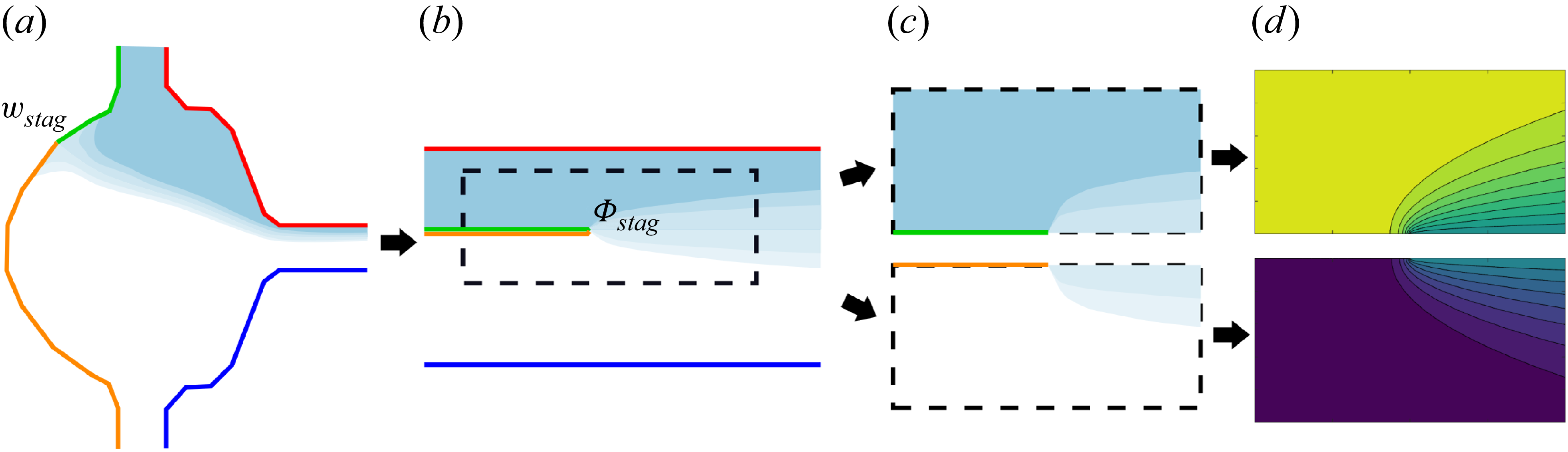
While the form of the equation is much simpler, in the general case, the problem in the streamline coordinate domain might have one or several mixed boundary conditions, which can be difficult to deal with. We first describe the construction of the solution for the simpler case of two inlets and one outlet.
Illustration of the construction of the solution in the streamline domain. (a) Mixer geometry
 $w$
. (b) Streamline coordinate domain problem. (c) Two halves of the streamline problem for high
 $\textit{Pe}$
, in which the outer walls are neglected. (d) Two leading edge similarity solutions to be patched together.

In the problem of two inlets of unequal flow rates, the streamline coordinate problem maps to two strips of different concentrations, each with a height of
 $k_i \pi$
. The strips are initially separated by a no-flux boundary which ends at a point
 $\varPhi _{\textit{stag}}$
, then allowed to mix with one another (see figure 3). The point
 $\varPhi _{\textit{stag}}$
corresponds to the image of the stagnation point located between the two point sources in the
 $\nu$
domain. This stagnation point’s position is given by
 \begin{equation} \nu _{\textit{stag}} = \frac {k_1 \nu _2 + k_2 \nu _1}{k_1 + k_2} \end{equation}
and its image in the
 $\varPhi$
domain is
 \begin{equation} \varPhi _{\textit{stag}} = k_1 \ln ( \nu _{\textit{stag}} - \nu _1) + k_2 \ln ( \nu _{\textit{stag}} - \nu _2). \end{equation}
The presence of the mixed boundary condition separating the two strips significantly complicates the problem; however, in the case of high-Péclet-number flows, it is possible to cut up the problem into a number of simpler subdomains and use this subdivision to construct solutions which are valid everywhere. In a high-Péclet-number regime, the mixing region will be confined to a thin wake originating at
 $\varPhi _{\textit{stag}}$
and of thickness
 $\sqrt {( {\phi - \phi _{\textit{stag}}})/{\textit{Pe}}}$
. As long as the thickness of this wake is small compared with the width
 $k_i \pi$
of the strip in the streamline domain, the effect of the no-flux boundaries at the top and bottom of the strip (red and blue segments in figure 3
b) will be negligible. Neglecting the outer boundary conditions in the streamline domain, we are left with the problem of an infinite domain with a different prescribed value of
 $c$
at infinity on each half-plane (dotted box in figure 3
b). The two half-planes are separated by a semi-infinite no-flux boundary that ends at
 $\varPhi _{\textit{stag}}$
. In this subdomain, the problem is symmetrical and the concentration on the separating axis, past
 $\varPhi _{\textit{stag}}$
, can be taken to be just the average of the two inlet concentrations.
We can finally split the problem into two simpler sub-problems (see figure 3
c). In each ‘half’ of the subdivided problem, we have a problem of advection–diffusion in plane flow in a semi-infinite domain, with a symmetry condition on half of the real axis, a prescribed concentration of
 $c = 1/2$
on the other half of the real axis and a concentration that tends to either 0 or 1 as
 $\lvert \varPhi \rvert \rightarrow \infty$
. The problem has thus been reduced to the classical boundary layer for uniform flow past a semi-infinite slipping flat plate. This problem can be solved in parabolic coordinates and has a simple similarity solution in terms of error functions (Cummings et al. Reference Cummings, Hohlov, Howison and Kornev1999; Bazant Reference Bazant2004). We can patch the two halves of the solution together to obtain an expression for the concentration field:
 \begin{equation} c \left ( \varPhi \right) = \begin{cases} \frac {1}{2} \left ( 1 - \text{erf} \left ( \text{Im} \sqrt { \textit{Pe} \left ( \varPhi - \varPhi _{\textit{stag}} \right) } \right) \right)\!, & \psi \lt 0, \\ \frac {1}{2} \left ( 1 + \text{erf} \left ( \text{Im} \sqrt { \textit{Pe} \left ( \varPhi - \varPhi _{\textit{stag}} \right) } \right) \right)\!, & \psi \geqslant 0. \\ \end{cases} \end{equation}
This solution has the familiar square root scaling of boundary layer thickness for slipping plates, which would be recuperated by using classical boundary layer analysis. Such a method of patching solutions together that appear on opposite sides of a separating streamline has been done in the past by Bazant & Moffatt (Reference Bazant and Moffatt2005) in constructing solutions to the Navier–Stokes equation with steady vortex structures. The novelty here lies in the shifting of the potential between the two half-plane solutions using
 $\varPhi _{\textit{stag}}$
. This shifting of the solutions becomes non-trivial when constructing more elaborate solutions where more than two subdomains are patched together, such as happens when analysing multiple inlets (see § 2.6). In that case, multiple stagnation points appear and different parts of the solution have their potential shifted by different values of
 $\varPhi _{\textit{stag}}$
.
The solution (2.15) breaks down when
 $\sqrt {({\phi - \phi _{\textit{stag}}})/{\textit{Pe}}}$
becomes comparable to the strip width
 $k_i \pi$
, at which point, the neglecting of the outer boundaries is no longer justified and the assumption that the separating line has a constant concentration, which is the average of the two inlet concentrations, is no longer true. In a previous publication, we have shown how a solution for this far-field regime can be obtained in terms of Green’s functions (Boulais & Gervais Reference Boulais and Gervais2020).
2.6. Multiple inlets solution
The procedure for solving the diffusion problem in mixers with more than two inlets is similar to the above-mentioned one, but involves a patching together of more than two similarity solutions. In multi-inlet mixers, the streamline domain
 $\varPhi$
corresponds to a series of strips of different concentration, initially separated by boundaries across which concentration cannot pass, and put in contact at different points (see figure 4).
Schematic of the different domains involved in the multi-inlet problem (the intermediate disk domain
 $z$
is not pictured). By slicing the domain along the red dotted lines, the problem can be subdivided into a sequence of smaller problems whose solution is given by (2.15). The solution breaks down when the wake’s width becomes comparable to the distance between dotted lines, or to the width of the smallest strip segment.

Like in the two-inlet case, identification of the stagnation points’ image in the
 $\varPhi$
domain is important, as they represent the end of the semi-infinite boundaries initially separating the different strips. There is a stagnation point in between each pair of point sources in the
 $\nu$
domain. While analytical determination of each stagnation point’s position is cumbersome when there are more than two apertures, there are a number of simple ways to approximate their positions.
-
(i) Numerically solve the equation
 $\boldsymbol{\nabla }\varPhi ( \nu) = {\boldsymbol{0}}$
to find the position of each stagnation point.
-
(ii) Use the weighed average of each pair of inlets to find the stagnation point between them. This assumes that the effect of the other inlets is mostly screened out by the two nearest singularities and the error committed in that case should be minimal.
-
(iii) If the mixer geometry has relatively sharp corners (such as illustrated in figure 8 c) and the ratio of the different injection rates are not too big, we can approximate that the position of the stagnation point will correspond to the image of the corresponding corner.

The solution will be a patchwork of wakes, each translated by the position of their respective stagnation point.
2.7. Multiple outlets
The solution procedure gets more complicated if there are multiple outlets. In problems with multiple outlets, the fluids of different concentration can be put in contact for a finite distance, then reseparated. In such a geometry, the mixing region can be confined to a strip of finite length, requiring more complex solution procedures. Such a finite strip problem (Pearson Reference Pearson1957) has been studied using combinations of numerical and analytical methods in problems of solidification in potential flows (Choi et al. Reference Choi, Margetis, Squires and Bazant2005). In microfluidics, classic H-filter systems (Weigl & Yager Reference Weigl and Yager1999) as well as microfluidic surface shields (Boyadjian, Boulais & Gervais Reference Boyadjian, Boulais and Gervais2022) involve such a streamline domain, where the finite strip solution needs to be used.
2.8. Schwarz–Christoffel maps
A key step in the derivation of our solution is the computation of the Schwarz–Christoffel map 2.9 between the complex polygonal mixer and disk domain. This map has a number of unknown
 $z_k$
parameters, which are the images of the vertices of the polygon in the disk domain, distributed along the circumference of the unit circle in the
 $z$
domain. With the exception of some limited cases with small numbers of vertices or high symmetry, the integral in (2.9) usually does not have a closed expression in terms of simple functions. However, its value at any point in the domain can easily be computed using numerical quadratures. The main difficulty in computing (2.9) is in determining the set of parameters
 $z_k$
, which is usually called the ‘parameter problem’, and is the more laborious part in computing complex Schwarz–Christoffel maps. The parameters
 $z_k$
are not known a priori and have to be determined by numerically solving a nonlinear system of equation, based on the constraints of our geometry. The method is in that sense semi-analytical. Various numerical methods for the generation of Schwarz–Christoffel maps (and the resolution of the parameter problem) have been presented throughout the years (Menikoff & Zemach Reference Menikoff and Zemach1980; Stephenson Reference Stephenson2005; Marshall & Rohde Reference Marshall and Rohde2007); this work implements the method described by Trefethen (Reference Trefethen1980). We outline the complete procedure in Appendix A. Despite adding a numerical step to our procedure, there is still advantage to using this method over simply numerically solving the transport problem from the start. Indeed, the set of pre-vertices
 $z_k$
only has to be computed once for a given geometry and can then be considered as known. This means that once the problem is solved for a given mixer shape, solutions to our flow and diffusion problem can be generated instantly for any combination of the problem parameters, without requiring additional numerical steps. This is useful in typical microfluidic applications, where the geometry of the mixer is unlikely to change in between experiments.
2.9. Inverting the map
Once the parameter problem has been solved and we know the set of parameters
 $z_k$
, the forward map
 $w(z)$
can be directly evaluated using (2.9). An illustration of a map to the interior of the mixer is shown in figure 5. However, evaluation of the concentration profile (2.15) for a given point
 $w$
in the mixer requires an expression of the inverse map
 $z(w)$
. To invert
 $w( z)$
, we differentiate, then take the multiplicative inverse of (2.9). This gives
 \begin{equation} \frac {{\rm d} z}{{\rm d} w} = \frac {1}{C} \prod _{k=1}^{n} \left ( 1 - \frac {z}{z_k} \right)^{1-\alpha _k}, \end{equation}
which is an ordinary differential equation (ODE) of the form
 \begin{equation} \frac {{\rm d} z}{{\rm d} w} = g (w, z). \end{equation}
Map
 $w ( z)$
from (a) the disk to (b) the interior of the mixer. The map is illustrated by displaying a regular polar grid in the
 $z$
domain and visualising its image in the
 $w$
domain. The vertices and their image in the disk domain are shown as black circles.

This equation can readily be integrated using a prepackaged ODE solver, provided we know the value of
 $z(w)$
at a given starting point. We use Matlab’s prepackaged ‘ode45’ solver for this calculation, which allows us to get the inverse map everywhere in the domain at a reasonable accuracy. If more accuracy is needed, Newton iterations can be used to refine the map. Newton iterations yield more precise end results, but require a reasonably accurate initial guess, which the ODE solver provides.
2.10. Complete procedure
We are now in a position to completely solve the 2-D diffusion problem in our microfluidic mixer. We summarise the steps to obtain analytical flow and concentration profiles in arbitrary polygonal mixers. This sequence is not trivial, as the different maps involved in building the solution require parameters computed in previous steps. The steps are as follows.
-
(i) Solve the pre-vertice problem for the Schwarz–Christoffel map from the disk to the interior of the mixer.
-
(ii) Compute the inverse map
$z ( w)$
on a grid of points in a region of interest. -
(iii) From the solution of the pre-vertice problem, obtain the values of
$z$
for the inlet and outlet vertices. -
(iv) The image of the outlet
$z_0$
allows computation of the Moebius transform (2.10), which gives an expression for
$\nu ( z)$
. -
(v) Applying the Moebius transform to the pre-vertices
$z_1$
and
$z_2$
of the inlets gives
$\nu _1$
and
$\nu _2$
, which go in the expression of the complex potential
$\varPhi ( \nu)$
, given in (2.11). -
(vi) The sequence of transforms
$\varPhi ( \nu)$
,
$\nu ( z)$
,
$w ( z)$
can be combined to evaluate the complex potential
$\varPhi ( w)$
at any point in the interior of the mixer. -
(vii) The potential
$\varPhi ( w)$
at any point in the mixer can be substituted in (2.15) to obtain the concentration at that point.


3. Results
3.1. Streamline plots
Streamlines in the microfluidic mixer can be plotted in two different ways. The first is to plot the streamlines in the z domain (interior of the disk), using (2.11) and (2.10). Individual points of these streamlines can then be mapped to the interior of the mixer by using the direct transform (2.9). This has the disadvantage of yielding varying resolution in the resulting streamlines, depending on the scale factor at different points in the map. In particular, this method makes it difficult to get accurate streamlines in highly elongated regions such as near the inlets and outlets. The second method of tracing the streamlines is to use the inverse map
 $z ( w)$
, which we calculated in § 2.9. Using the inverse map, we can directly find the value of the complex potential
 $\varPhi ( \nu ( z ( w))) = \varPhi ( w)$
at any given point in the
 $w$
domain. Provided we have evaluated
 $z ( w)$
for a sufficient number of points in our region of interest, we can then just find the level sets of the real or complex part of
 $\varPhi ( w)$
using a built-in function such as Matlab’s contour plot. This second method is used to obtain the streamline maps illustrated in figure 6.
Streamlines (blue) and potential level set (red) in the microfluidic mixer for different ratios of inlet flow rates. The flow from the left inlet has been coloured light blue for additional clarity. (a) 1–1 inlet ratio. (b) 1–3 inlet ratio. (c) 1–8 inlet ratio.

3.2. Concentration plots
The inverse map
 $z ( w)$
computed in § 2.9 allows us to evaluate the complex potential
 $\varPhi ( w)$
for any point in our domain. From this complex potential, we can then evaluate the diffusion solution in the streamline coordinate domain (2.15). This allows us to instantly evaluate the concentration at any given point
 $w$
in the domain, provided we have already precomputed the inverse map at that point. We use this method to trace concentration maps for various values of the Péclet number, illustrated in figure 7. In figure 8, we show streamline as well as concentration plots obtained for a variety of geometries, reminiscent to diverse previously published microfluidic mixers. This showcases the versatility of the approach and its adaptability to arbitrary geometries. Additional figures for multi-inlet mixer geometries are shown in Appendix B.
Concentration profile in polygonal mixer with a 1–3 injection ratio for different Péclet number: (a)
 $\textit{Pe} = 10$
; (b)
 $\textit{Pe} = 100$
; (c)
 $\textit{Pe} = 1000$
.

(a,b,c) Streamline profiles and (d,e, f ) concentration fields in various polygonal mixers: (a,d) Y junction with unequal injections (Gobby et al. Reference Gobby, Angeli and Gavriilidis2001); (b,e). hydrodynamic focusing reminiscent of (Knight et al. Reference Knight, Vishwanath, Brody and Austin1998); (c, f ) hydrodynamic focusing system with five inlets (Park et al. Reference Park, Qiu, Rhoades, Korlach, Kwok, Zipfel, Webb and Pollack2006).

3.3. Physical tracer tests
To validate the results, we compare predicted concentration profiles to experimental physical tracer tests done by injecting blue dye in a microfluidic analogue to an impinging jet mixer. The results are presented in figure 9. We find excellent agreement between predicted and experimental results.
Comparison with physical tracer tests: (a,b,c) predicted concentration profiles for flow ratios of 1–1, 1–1.8 and 3–1, each with Péclet number 1000; (d,e, f ) matching physical tracer tests in microfluidic mixer using blue dye. Scale bar, 100
 ${\mu}$
m.

3.4. Cross-flow geometries
In addition to mixer geometries, our methodology can be used to model other polygonal microfluidic devices. In particular, cross-flow geometries have been used in a number of microfluidic applications, from the reproduction of G.I. Taylor’s classic four-roll mill (Lee et al. Reference Lee, Dylla-Spears, Teclemariam and Muller2007) to the creation of adjustable hydrodynamic traps (Tanyeri, Johnson-Chavarria & Schroeder Reference Tanyeri, Johnson-Chavarria and Schroeder2010) to applications in microrheology (Haward et al. Reference Haward, Oliveira, Alves and McKinley2012). In such systems, alternating inlets and outlets are used to generate tuneable extensional flows in microfluidic chambers. We show in figure 10 how our framework can be used to rapidly model flow and diffusion in one such existing system: the microfluidic rheometry system presented by Haward et al. (Reference Haward, Oliveira, Alves and McKinley2012). Analysis of such systems is usually done either by numerically solving the full Stokes flow problem or by only focusing on a region of interest around the stagnation point. Our method provides an elegant alternative, which takes into account the entire geometry and allows for rapid generation of flow or concentration profiles once a map to the interior of the chamber has been found.
Analysis of an extentional flow rheometry system similar to that of Haward et al. (Reference Haward, Oliveira, Alves and McKinley2012). (a) Schwarz–Christoffel map to the interior of the chamber. (b) Streamline profile for equal injection and aspiration flow rates. (c) Resulting concentration profile for
 $\textit{Pe} = 50$
.

4. Discussion
4.1. Avenues for applications
One immediate application of the models thus developed is in the determination of residence time distribution curves, which are an important element of the experimental characterisation of chemical reactors (Levenspiel Reference Levenspiel1998). Neglecting diffusive effects, residence time distribution can be obtained directly by integrating along the streamlines of the flow. Residence time distributions that consider diffusive effects (which are particularly relevant in microfluidic systems, due to the importance of Taylor dispersion) can be obtained by a combination of integration along streamlines in the
 $xy$
plane and Monte Carlo methods to model diffusion along the
 $z$
axis, similar to what is done by Houseworth (Reference Houseworth1984). In systems that are very thin, we expect Taylor dispersion effects to be predominant, which will give heavy tails to residence time distribution curves. While microfluidic systems are often transparent and experimental probing of the flow within them is better done using techniques such as microparticle image velocimetry (
 $\mu$
PIV), the determination of residence time distribution curves is an essential element when probing opaque systems. Computation of residence time distributions may also be a way to extend the methods from the present article to other systems, namely macroscopic flows in groundwatersheds (Haitjema Reference Haitjema1995), wetlands (Werner Reference Werner and Kadlec2000) or river beds (Gooseff et al. Reference Gooseff, Benson, Briggs, Weaver, Wollheim, Peterson and Hopkinson2011), where the flow may still be approximated using potential flow theory, but direct imaging of the flow by PIV or other visual methods is much more difficult.
Similar Monte Carlo simulations, combined with knowledge of the concentration at every point in the mixer, could be used to simulate the trajectory of individual particles in the mixer and determine their microenvironment at every time step (in a typical flash nanoprecipitation experiment, this could include both the concentration of solvent versus antisolvent as well as the temperature, if the different inlets had different initial temperatures). This precise knowledge could then be combined with the population balance model, or other more elaborate models of particle growth kinetics, to predict the output product in different types of flash nanoprecipitation experiments (Saad & Prud’homme Reference Saad and Prud’homme2016) in microfluidic mixers. This is a crucial next step in the use of microfluidic mixers for pharmaceutical applications, especially for lipid nanoparticles, and will be elaborated on in future publications.
4.2. Limitations
The models that we develop in this article hinge on a number of assumptions about our flow profile. In particular, they neglect eventual 3-D effects in the flow. The Hele-Shaw cell formulation is valid at low enough Reynolds numbers and assumes that the flow everywhere can be described by a 2-D potential flow in the
 $xy$
plane, modulated by a parabolic profile in the
 $z$
direction. This approximation eventually breaks down in mixers where the height is comparable to the characteristic dimension in the
 $xy$
plane, as the Reynolds number is increased. This can be seen in analysis of T-mixers, where increasing Reynolds number moves the system from a stratified flow regime first to a vortex regime, where vortices appear along the cross-section, then a so-called engulfment regime, where flow symmetry is broken (Fani, Camarri & Salvetti Reference Fani, Camarri and Salvetti2013). Similar effects also lead to trapping of particles in T-junctions (Vigolo, Radl & Stone Reference Vigolo, Radl and Stone2014). These regimes are important to analyse, as mixing is significantly improved in the engulfment regime. However, these are much more difficult to assess analytically, and state-of-the-art models for these situations usually involve a combination of scaling arguments and direct numerical simulation of the Navier–Stokes equations. Similar 3-D effects along the cross-section are also responsible for much of the mixing in many types of chaotic mixers (Stroock et al. Reference Stroock, Dertinger, Ajdari, Mezic, Stone and Whitesides2002), which are commonly used in microfluidic mixing experiments. Extensive work on the theoretical foundations of mixing in these ‘stretch-and-fold’ chaotic mixers have been laid out, and we refer the reader to the pioneering work of Ottino (Reference Ottino1989), Ottino & Wiggins (Reference Ottino and Wiggins2004) and Aref (Reference Aref1984) for more information on the subject.
4.3. Possible extensions
The analytical method developed in this article could be extended in several ways. We mentioned earlier the use of Schwarz–Christoffel maps for the generation of grids, which could then be used to develop numerical methods for the analysis of flow in complex geometries (Thompson, Warsi & Mastin Reference Thompson, Warsi and Wayne Mastin1982). The method of conformal transforms that we employ is also applicable to some other systems of equations, beyond the simple advection–diffusion in potential flow described throughout this article. In particular, a similar procedure could be applied to dilute electrolyte solutions, in which the concentration field is also affected by a mobility term proportional to the gradient of an electric potential
 $\boldsymbol{E} = - \boldsymbol{\nabla }V$
(Bazant Reference Bazant2004). In particular, a similar conformal mapping procedure has been used in the study of microfluidic electrodeposition (Gu et al. Reference Gu, Huo, Xu, Su, Bazant and Deng2022). The method could also be applied to problems of flow and diffusion in porous media, specifically in planar aquifers or in problems of hydrocarbon recovery (Koplik et al. Reference Koplik, Redner and Hinch1994). In such problems, our method would allow the precise determination of residence times for Brownian tracers in complex polygonal domains. The method could also easily be extended to domains with variable permeability, using methods outlined by Strack (Reference Strack1988). The extension of the method to problems of transport in porous media also suggests uses in studying transport in hydrogels, porous biological samples or in paper microfluidics (Müller & Clegg Reference Müller and Clegg1949; Martinez et al. Reference Martinez, Phillips, Butte and Whitesides2007).
The method could very simply be modified to solve problems of steady-advection–diffusion around the exterior of regular polygons. This could yield very interesting results applicable to problems of dissolution (Rycroft & Bazant Reference Rycroft and Bazant2016) or in the analysis of diffusion-limited crystallisation around polygonal grains (Seeger Reference Seeger1953), two areas of transport where similar complex variable methods have been used in the past.
5. Conclusion
We present versatile models for flow and diffusion in microfluidic mixers of arbitrary polygonal shapes, based on Schwarz–Christoffel maps. The models yield values for flow field as well as 2-D-averaged concentration profile everywhere in the geometry. Such models are general and applicable to a range of microfluidic system, in particular, in mixers used for the synthesis of complex nanomaterials, specifically lipid nanoparticles. In this context, a complete knowledge of the microhistory of individual particles (such as is afforded by our models) is a key element in the probing of the kinetics of the particles’ self-assembly and should open the way to better knowledge-based methods of synthesis. Beyond this direct application, the mathematical framework we have presented can also find application in other domains, namely transport in porous media, groundwater mechanics or magnetohydrodynamics, to name a few.
6. Method
6.1. Computation
Results were generated using custom code written in Matlab R2018a. The nonlinear equation system involved in determining the pre-vertices was solved using the pre-packaged fsolve method. Inversion of the map was performed using the pre-packaged ODE45 solver. Coefficients for the Gauss–Jacobi quadratures, used in calculating the integrals, were determined with custom code using the method of Golub & Welsch (Reference Golub and Welsch1969).
6.2. Experimental
A microfluidic chip which geometrically mimics an impinging jet mixing design was fabricated in polymethyl methacrylate using transition moulding (Parallel Fluidics, USA). The dimensions of the chip are shown in figure 11. Threaded ports were securely bonded to both the inlet and outlet of the chip. The chip’s inlet and outlet were connected to fittings (IDEX) and PTFE tubing (inner diameter, 0.5 mm; outer diameter, 1 / 16”, IDEX). The inlet tubing was connected to two syringe pumps (SyringeONE NE-1000, New Era Pump Systems Inc.), while the outlet tubing was connected to a waste collection vial. Two solutions were mixed within the microfluidic chip: Milli-Q water and an aqueous solution of Methylene Blue (100 mg L−1). Methylene Blue (minimum 82 % dye content), purchased from Fisher Scientific, was used without further purification. Mixing behaviour was recorded using a colour CMOS camera (DFK 22BUC03, The Imaging Source) mounted on a Nikon Eclipse E20 microscope. The mixing zone was illuminated from below using a halogen light source (HL 150-B) with a flexible arm for optimal positioning. Images were captured at 30 frames per second with a resolution of 1288
 $\times$
922 pixels. Experiments were run with flow rate ratios varying from 1:1 to 10:1, with an inlet flow rate
 $Q_0$
of 25
 ${\mu}$
l min−1. Using the standard expressions
 ${Re} =({\rho u L}/{\mu })$
and
 $\textit{Pe} = ( {Q_0}/{2 \pi G D})$
gives Reynolds numbers
 ${Re} \approx 0.5$
and Péclet numbers
 $\textit{Pe} \approx 1000$
. We are thus squarely in the low-Reynolds, high-Péclet regime demanded for our approximations to hold.
Dimensions of the microfluidic device that mimics an impinging jet mixer design. The depth of the device is 100
 ${\mu}$
m.

Funding
This research is funded by the U.S. Food and Drug Administration under the FDA BAA-22-00123 program, Award Number 75F40122C00200. E.B. acknowledges funding from the Fond de Recherche du Quebec, Nature et Technologie (FRQNT) Postdoctoral Fellowship Program, as well as National Science and Engineering Research Council of Canada (NSERC) Postdoctoral Fellowship Program
Declaration of interests
The authors report no conflicts of interest.
Appendix A. Computation of the Schwarz–Christoffel map
The Schwarz–Christoffel map
 \begin{equation} w \left ( z \right) = w_c + C \int ^z \prod _{k=1}^{n} \left ( 1 - \frac {\xi }{z_k} \right)^{\alpha _k - 1} \,{\rm d} \xi \end{equation}
has a number of unknown parameters
 $z_k$
, which are the image of the vertices of the polygon in the disk domain. These are unknown a priori and have to be determined as part of the solution procedure. There are different ways of formulating the parameter problem. We follow the procedure outlined by Trefethen (Reference Trefethen1980). The Riemann mapping theorem technically lets us freely determine three of the
 $z_k$
, and some sources fix three pre-vertices and then define
 $n - 3$
equations to find the other (Driscoll Reference Driscoll2002). Instead of doing this, we fix a single one and add an additional condition for the image of the disk’s origin. This means we are solving a system of
 $n - 1$
equations for the pre-vertex problem (instead of
 $n - 3$
equations if we had fixed three pre-vertices). Doing so allows us to have a better distribution of pre-vertices around the circle and avoid crowding and the numerical instabilities that come with it (see Appendix A.4 for an illustration of this). The equation for the position of the centre point is
 \begin{equation} w_1 - w_c = C \int _{0}^{z_1} w^{\prime} ( \xi)\,{\rm d} \xi . \end{equation}
Equation (A2) is a complex equation, whose real and imaginary part give two real equations for our system. For the remaining
 $n - 3$
equations, we use the polygon’s side lengths,
 \begin{equation} \frac {\big |{\int _{z_j}^{z_{j+1}} w^{\prime} ( \xi) \,{\rm d} \xi }\big |}{\lvert \int _{z_1}^{z_2} w^{\prime} ( \xi) \,{\rm d} \xi \rvert } = \frac {\lvert w_{j+1}-w_j \rvert }{\lvert w_2-w_1 \rvert }. \end{equation}
In the case of vertices at infinity (for example, the end of the inlet and outlet channels), we have two infinite side lengths, for which the real (A3) cannot be used. We use instead the complex equation
 \begin{equation} \frac {\int _{z_{j-1}}^{z_{j+1}} w^{\prime} ( \xi)\, {\rm d} \xi }{\big |{\int _{z_1}^{z_2} w^{\prime} ( \xi)\, {\rm d} \xi }\big |} = \frac {w_{j+1}-w_{j-1}}{\lvert w_2-w_1 \rvert }, \end{equation}
where
 $w_j$
is a vertex at infinity. The real and imaginary parts of (A4) give two real equations for each vertex at infinity. Equations A2, A3 and A4 thus give a system of
 $n - 1$
equations which can be solved to obtain the values of
 $z_k$
, completing the parameter problem. The remaining parameter
 $C$
can be obtained by normalising with the length of one of the edges. Put succinctly, the pre-vertex problem consists of passing from a description of our geometry in terms of a list of interior angles and side lengths (which is immediately available to us) to one in terms of a list of interior angles and a list of positions of the pre-vertices
 $z_i$
around the unit circle, which can then be plugged directly in (2.9).
A.1. Calculating the integrals
Equation (2.9), which is used to compute the map, as well as (A3) and (A4) used for solving the parameter problem, require the evaluation of complex integrals. Since the function
 $w ( z)$
is analytic everywhere inside of the disk, the value of the integrals is path-independent and we can calculate them along straight line segments. Precise computation of these integrals is difficult when the endpoints are pre-vertices, as the integrand of (2.9) is singular at these points. The presence of singularities at the endpoints of the integrals means traditional Newton–Cotes or Gauss–Legendre quadratures behave very poorly. This is of importance not only in calculating the Schwarz–Christoffel map, but also in solving the pre-vertex problem, as imprecise integrals will also limit the possible precision with which the parameter problem can be solved. Since pre-vertices also have a tendency to crowd in elongated regions (Driscoll Reference Driscoll2002), insufficient precision in the integrals can easily lead to parameter problems that fail to converge to a solution. To circumvent this issue, we follow Trefethen (Reference Trefethen1980) and use compound Gauss–Jacobi quadratures for the integrals with endpoint singularities (Davis & Rabinowitz Reference Davis and Rabinowitz2007). The coefficient for these quadratures are obtained by implementing the method of Golub & Welsch (Reference Golub and Welsch1969), which is based on finding the eigenvalues of a matrix constructed from the recurrence rule of orthogonal polynomials (in this case, Jacobi polynomials). The recurrence rules for Gauss–Jacobi polynomials can be found in classic treatises on orthogonal polynomials (Szego Reference Szego1939). Variations of Newton–Cotes quadratures that account for the presence of endpoint singularities also exist and could have been used instead (Floryan & Zemach Reference Floryan and Zemach1988).
A.2. Solving the parameter problem
Once we have a method for efficient calculation of the integrals, we are almost set to solve the parameter problem. Equations A3 and A4 define a nonlinear algebraic problem. The pre-vertices
 $z_k$
are distributed around the unit circle and thus can be written as
 \begin{equation} z_k = e^{i \theta _k} \end{equation}
with
 $0 \lt \theta _k \lt 2 \pi$
and
 $\theta _1 \lt \theta _2 \lt \ldots \lt \theta _n$
. The problem of the determination of
 $\theta _k$
is thus a constrained one and, as such, is significantly more difficult to solve numerically than an unconstrained one. To bypass this difficulty, Trefethen (Reference Trefethen1980) suggests the change of variable
 \begin{equation} y_k = \text{log} \frac {\theta _k - \theta _{k-1}}{\theta _{k+1} - \theta _k} \end{equation}
with
 $\theta _0$
and
 $\theta _k$
taken as
 $0$
and
 $2 \pi$
, respectively, both representing the argument of
 $z_k$
. The passage to an unconstrained nonlinear algebraic problem allows us to use any one of a number of robust ‘black-box’ numerical solvers. We use Matlab’s built-in ‘fsolve’ function, which is based on a standard algorithm by Powell which combines Newton iterations and steepest descent (Powell Reference Powell1968). This method allows for the resolution of problems with 30 to 100 vertices in relatively short times, of the order of minutes on a standard laptop computer.
A.3. Extension to channel geometries
The method presented previously involves a transformation from a disk domain to the interior of our polygonal mixer. This method yields precise results for the interior of mixers where the dimensions of the domain are comparable in both the
 $x$
and
 $y$
directions, but may become unprecise for highly elongated geometries. More specifically, transforming from a disk is not ideal when mapping to long channel-like geometries. Transformation from the disk is also unsuitable for mapping infinite periodic geometries, such as zigzagging channels (Mengeaud, Josserand & Girault Reference Mengeaud, Josserand and Girault2002) or baffled micromixers (Kimura et al. Reference Kimura, Maeki, Sato, Note, Ishida, Tani, Harashima and Tokeshi2018). To model such geometries, it is more appropriate to use an infinite strip as our
 $z$
domain. Such a map is described by Floryan (Reference Floryan1985). The procedure in that case is exactly the same, but the map in (2.9) is replaced with
 \begin{equation} w ( z) = w_c + C \int ^z \prod _{k=1}^{n} \left ( \text{sinh} \frac {\pi }{2} ( \xi - z_k) \right)^{\alpha _k - 1}\, {\rm d} \xi . \end{equation}
Additional care must be taken to ensure that, in addition to being correctly ordered, the pre-vertices are on the correct side of the strip. While maps can be found to the interior of 2-D channel-like systems such as zigzag mixers or baffled micromixers, it is important to remember that most of the actual mixing done in these geometries comes not from passive lateral mixing in potential flow, but from effects that are not captured in our current models. Namely, mixing in these geometries depends on 3-D aspects of the flow, on recirculations caused by the interaction of sharp corners and the viscous boundary layers, and on the chaotic aspects of the flow thus generated. That being said, mapping to periodic channel geometries may still be useful for grid generation in the context of numerical analysis, as well as for generating first-order solutions on top of which more complex transport models may be elaborated. For more details on channel geometries, we refer the reader to Floryan (Reference Floryan1985), who describes the procedure for channel geometries in detail. We do note that their article uses a different notation from ours, with the pre-vertex domain labelled as
 $w$
and the physical flow domain as
 $z$
rather than the other way around.
A.4. Fixing pre-vertices
Effect of fixing pre-vertices. (a) Disk domain when the position of the last three pre-vertices is fixed at
 $z_{n-2}=-1$
,
 $z_{n-1}=-i$
,
 $z_n=1$
. (b) Map to the interior of the mixer when three pre-vertices are fixed. (c) Disk domain when a single pre-vertex is fixed
 $z_n=1$
and the image of the origin is prescribed. (d) Map to the interior of the mixer when a single vertex and the image of the origin are prescribed.

In figure 12, we show an illustration of the effect of the choice of pre-vertices on the Schwarz–Christoffel map. If we fix the position of the last three pre-vertices
 $z_{n-2}$
,
 $z_{n-1}$
and
 $z_n$
, as the Riemann mapping theorem allows us to do, we generally observe heavy crowding of the pre-vertices around the disk (see figure 12
a), which translates to a map with uneven scale factor, where some regions are very elongated and some are not (figure 12
b). In contrast, if we fix only a single pre-vertex and add an additional condition for the image of the centre of the disk in the mixer domain, we can obtain a more even distribution of pre-vertices around the circle and a map that is much more uniform (figure 12
c,d), which facilitates both the computation of the pre-vertex problem and the computation of the map and its inverse once the pre-vertex problem has been solved. Somewhat counterintuitively, despite the fact that the second case involves the resolution of a nonlinear system of
 $n-1$
equations instead of
 $n-3$
equations, the nonlinear system in the second case may actually converge faster because of the better conditioning of the problem.
Appendix B. Additional figures
In figure 13, we show more results for a multi-inlet solution with asymmetrical inlet injection rates. This shows that our methodology does not hinge on any particular symmetry of the problem.
(a,b,c) Streamline and (d,e, f ) concentration profiles in multi-inlet mixers for asymmetrical injection ratios.