





1. Introduction
Achieving and maintaining laminar flow on large swept surfaces of transport aircraft poses a considerable challenge for aerodynamic design. Surface roughness, for instance, contamination by insects and other debris, rivets or joints introducing sharp surface features, is a source of significant laminar flow deterioration. However, the boundary layer of aircraft-wing flow ought to remain laminar over the largest possible extent to reduce the viscous drag and, hence, the fuel consumption of the aircraft. To guide manufacturing tolerances for laminar wings and to develop transition-prediction methodologies, it is imperative to understand the influence of such surface features on flow instabilities and laminar breakdown.
Recent investigations on the topic (Tufts et al. Reference Tufts, Reed, Crawford, Duncan and Saric2017; Eppink Reference Eppink2020; Rius-Vidales & Kotsonis 2020, 2021, Reference Saric, Reed and White2022) focused on effects of two-dimensional (i.e. invariant in one spatial direction) forward-facing steps on transition driven by the spatial amplification of the stationary crossflow instability (CFI). In this context, the literature distinguishes three transition regimes induced by a forward-facing step, according to the upstream shift of the transition front: a negligible shift, a notable shift and an abrupt shift to a location immediately downstream of the step. The present work investigates theoretically and numerically the third regime, in which the step produces an abrupt upstream shift of the transition front. To this end, the pertinent flow structures are examined.
1.1. The CFI
Stability analysis of boundary-layer flow typically deals with the evolution of initially small-amplitude perturbations on a reference laminar flow state, the so-called unperturbed base flow (Mack Reference Mack1984; Arnal Reference Arnal1993; Schmid & Henningson Reference Schmid and Henningson2001; Theofilis Reference Theofilis2003). In this work the base flow is the three-dimensional boundary layer over a swept wing. Laminar–turbulent transition is initiated by the exponential amplification of a primary stationary crossflow perturbation; this is the prevalent scenario in swept-wing flow subject to a low-disturbance environment as in free flight (Saric et al. Reference Saric, Reed and White2003). Deyhle & Bippes (Reference Deyhle and Bippes1996) discuss the receptivity conditions leading to dominance of the stationary (i.e. zero temporal frequency) or the travelling (i.e. non-zero temporal frequency) form of the CFI. The growth of a stationary CFI in the leading-edge-orthogonal (or chordwise) direction results in the amplification of so-called co-rotating stationary crossflow vortices. The axes of the crossflow vortices are approximately aligned with the direction of the streamlines in the outer-flow region (Bippes Reference Bippes1999; Haynes & Reed Reference Haynes and Reed2000).
The stationary vortical action of the CFI is responsible for the strong modulation of the boundary layer and consequent appearance of vigorous shear layers. These, in turn, give rise and sustain secondary instabilities, typically harbingers of laminar breakdown. Secondary instabilities are mainly classified based on their frequency content and location around the crossflow vortex as type I (or zmode), type II (or ymode) (Malik et al. Reference Malik, Li, Choudhari and Chang1999) and type III (Fischer & Dallmann Reference Fischer and Dallmann1991; Koch et al. Reference Koch, Bertolloti, Stolte and Hein2000). For further details on the behaviour of a secondary CFI, the reader is referred to the numerical work of, e.g. Högberg & Henningson (Reference Högberg and Henningson1998), Wassermann & Kloker (Reference Wassermann and Kloker2002) and Li et al. (Reference Li, Choudhari and Duan2016b ), the experimental work of, e.g. White & Saric (Reference White and Saric2005) and Serpieri & Kotsonis (Reference Serpieri and Kotsonis2016), and work on stability analysis of, e.g. Bonfigli & Kloker (Reference Bonfigli and Kloker2007) and Groot et al. (Reference Groot, Serpieri, Pinna and Kotsonis2018).
In recent years, an increasing number of studies have performed stability analyses of the secondary CFI using a non-orthogonal coordinate system (Li & Choudhari Reference Li and Choudhari2011; Casacuberta et al. Reference Casacuberta, Groot, Hickel and Kotsonis2022a ; Ambrosino et al. Reference Ambrosino, Tocci, Theiß, Hein and Rodríguez2025; Groot et al. Reference Groot, Casacuberta and Hickel2025). In this formulation, the spanwise axis is aligned with the wing’s leading edge, while the streamwise axis follows the direction of the stationary crossflow vortex. This choice both enforces spanwise periodicity and naturally incorporates the assumption of slow flow variation along the crossflow-vortex direction.
1.2. Alternative routes to transition beyond modal instability
Morkovin (Reference Morkovin1969) introduced the notion that a primary instability mechanism, such as a CFI, can be bypassed by ‘another strongly amplifying mechanism’. Throughout the years, the idea of a bypass transition has been subject to debate, especially under the influence of surface features. Nonetheless, the existence of alternative routes towards transition is presently well established (Reshotko Reference Reshotko2001).
Ellingsen & Palm (Reference Ellingsen and Palm1975) demonstrate that for an initial three-dimensional perturbation in an inviscid shear layer (i.e. neglecting the viscous term in the perturbation equation) its streamwise component may grow linearly (or algebraically, as opposed to exponentially) in time by generating streaks, namely, alternating regions of high- and low-speed fluid. Landahl (Reference Landahl1975, Reference Landahl1980) further elaborated on the linear mechanism producing the streaks, a process now commonly referred to as the lift-up effect. Algebraic perturbation growth has been ascribed mathematically to the non-normality of the linear operator governing the evolution of perturbations, i.e. the non-orthogonality of its associated eigenfunctions (Butler & Farrell Reference Butler and Farrell1992; Trefethen et al. Reference Trefethen, Trefethen, Reddy and Driscoll1993; Reddy & Henningson Reference Reddy and Henningson1993; Schmid & Henningson Reference Schmid and Henningson2001).
Similar to the classic stationary CFI, sufficiently amplified streaky structures can sustain secondary instabilities (Andersson et al. Reference Andersson, Brandt, Bottaro and Henningson2001; Asai et al. Reference Asai, Minagawa and Nishioka2002; Brandt et al. Reference Brandt, Cossu, Chomaz, Huerre and Henningson2003; Konishi & Asai Reference Konishi and Asai2004; Brandt Reference Brandt2007; Ricco et al. Reference Ricco, Luo and Wu2011), eventually leading to premature breakdown and transition, even if the streaks are predicted to decay asymptotically. This scenario typically arises in the wake of a critical three-dimensional surface feature in unswept conditions (De Tullio et al. Reference De Tullio, Paredes, Sandham and Theofilis2013; Loiseau et al. Reference Loiseau, Robinet, Cherubini and Leriche2014; Casacuberta et al. Reference Casacuberta, Groot, Ye and Hickel2020). It may also occur during what is most commonly understood as bypass transition, where so-called Klebanoff modes (Kendall Reference Kendall1985) develop in two-dimensional flow subjected to moderate-to-high levels of free-stream turbulence (Klebanoff Reference Klebanoff1971; Westin et al. Reference Westin, Boiko, Klingmann, Kozlov and Alfredsson1994; Matsubara & Alfredsson Reference Matsubara and Alfredsson2001; Jacobs & Durbin Reference Jacobs and Durbin2001; Brandt et al. Reference Brandt, Schlatter and Henningson2004; Zaki & Durbin Reference Zaki and Durbin2005). Analogous to the instability mechanisms associated to Görtler vortices (Swearingen & Blackwelder Reference Swearingen and Blackwelder1987), secondary instabilities of streaks are typically classified as either symmetrical (called varicose) or anti-symmetrical (called sinuous) based on their eigenmode shape relative to the streak shape. The spatial growth of sinuous and varicose instabilities leads to the shedding of quasi-streamwise-oriented vortices and hairpin-like vortices, respectively (Asai et al. Reference Asai, Minagawa and Nishioka2002; Brandt & Henningson Reference Brandt and Henningson2002; Konishi & Asai Reference Konishi and Asai2004).
Velocity streaks have been observed close downstream of a forward-facing step under both unswept (Stüer et al. Reference Stüer, Gyr and Kinzelbach1999; Wilhelm et al. Reference Wilhelm, Härtel and Kleiser2003; Marino & Luchini Reference Marino and Luchini2009; Lanzerstorfer & Kuhlmann Reference Lanzerstorfer and Kuhlmann2012) and swept (Casacuberta et al. Reference Casacuberta, Westerbeek, Sumariva, Groot, Hickel, Hein and Kotsonis2025) conditions and their origin has been attributed to the lift-up effect (Lanzerstorfer & Kuhlmann Reference Lanzerstorfer and Kuhlmann2012; Casacuberta et al. Reference Casacuberta, Westerbeek, Sumariva, Groot, Hickel, Hein and Kotsonis2025). The potential impact of such streaks on the mechanisms of transition advancement due to the step is at present not fully elucidated. It is presently well established that in swept-wing flow, the short-term algebraic growth of streaks can act as a precursor to the formation of crossflow vortices. Although the amplification of a CFI is primarily driven by a modal instability mechanism (see the discussion above), swept-wing flow supports significant non-modal growth of localised perturbations (Breuer & Kuraishi Reference Breuer and Kuraishi1994; Corbett & Bottaro Reference Corbett and Bottaro2001; Tempelmann et al. Reference Tempelmann, Hanifi and Henningson2010).
1.3. Transition advancement due to a forward-facing step
Historically, predictions of the threshold height of a surface feature influencing transition have relied on correlation parameters. The so-called roughness Reynolds number stands out in this regard,
 \begin{align} Re_{hh} = \frac {u_h h}{\nu }, \end{align}
where
 $h$
denotes the height of the feature,
 $\nu$
is the kinematic viscosity and
 $u_h$
expresses the velocity at the height of the surface feature in the unperturbed flow, i.e. without the surface feature; see, for instance, Smith & Clutter (Reference Smith and Clutter1959). For surface steps, correlations between the
 $Re_{hh}$
and the location of the transition front are provided by Drake et al. (Reference Drake, Bender, Korntheuer, Westphal, McKeon, Gerashchenko, Rohe and Dale2010) for an unswept flat plate with a prescribed favourable pressure gradient and by Duncan Jr. et al. (Reference Duncan, Crawford, Tufts, Saric and Reed2013) for a swept flat plate. However,
 $Re_{hh}$
does not serve as a universal predictive criterion and recent studies on steps have focused on elucidating the physical mechanisms governing laminar–turbulent transition.
Sketch of classic secondary crossflow instabilities. Isocontours of stability eigenmode shapes (40 %, 60 % and 80 % of maximum value) corresponding to type I (
 $5.2$
kHz and green), II (
 $8$
kHz and red) and III (
 $1$
kHz and blue) at
 $x/\delta _0 = 275$
for the large-amplitude case without a step (see
 $\S$
2.2) analysed in this work. Solid black lines are velocity isolines of the steady perturbed flow illustrating the stationary crossflow vortex.

Casacuberta et al. (Reference Casacuberta, Hickel and Kotsonis2021, Reference Casacuberta, Hickel, Westerbeek and Kotsonis2022b , Reference Casacuberta, Hickel and Kotsonis2024, Reference Casacuberta, Westerbeek, Sumariva, Groot, Hickel, Hein and Kotsonis2025) examined the stationary interaction between a forward-facing step and a pre-existing CFI, segregating two distinct processes. First, the upward displacement of the CFI as it approaches the step and passes over it, as also reported experimentally (Eppink Reference Eppink2020; Rius-Vidales & Kotsonis Reference Rius-Vidales and Kotsonis2021). Second, the rapid spatial amplification of stationary perturbation streaks near the wall, both upstream and downstream of the step. These streaks manifest as alternating high- and low-speed flow regions aligned along the step-edge (or wingspan) direction. Their structural identification aligns with previously reported instability characteristics at the step (Tufts et al. Reference Tufts, Reed, Crawford, Duncan and Saric2017; Eppink Reference Eppink2020; Rius-Vidales & Kotsonis Reference Rius-Vidales and Kotsonis2021). However, their potential role in promoting transition remains unexplored.
Tufts et al. (Reference Tufts, Reed, Crawford, Duncan and Saric2017) report the presence of a travelling mode in the region of local flow recirculation at the step, attributing the advancement of the transition front to its influence. Eppink (Reference Eppink2020) ascribes early transition to unsteady vortex shedding emanating from the deformed shear layer at the step which, in turn, is triggered by the growth of unsteady perturbations in the shear layer past the step. The role of classic secondary crossflow instabilities in promoting transition is deemed unlikely by Eppink (Reference Eppink2020). Rius-Vidales & Kotsonis (Reference Rius-Vidales and Kotsonis2022) experimentally measure significant temporal fluctuations on both the outer and inner sides of the lateral upward-inclined region of the stationary crossflow vortices past the step. These correspond respectively to the right-hand and left-hand sides in figure 1, which also highlights that the lateral upward-inclined region is dominated by the type-I instability. The scenario of abrupt transition at the step is linked to fluctuations originating from the inner side (Rius-Vidales & Kotsonis Reference Rius-Vidales and Kotsonis2022).
Rius-Vidales & Kotsonis (Reference Rius-Vidales and Kotsonis2022) note that, while these inner unsteady fluctuations originate in the region where the type-III secondary CFI develops, their measured frequencies are significantly higher than those of the type-III instability. Simultaneously, fluctuations on the inner side do not correlate spatially with the high-frequency type-I and type-II secondary crossflow instabilities (Rius-Vidales & Kotsonis Reference Rius-Vidales and Kotsonis2022). Together, these observations suggest a distinct unsteady mechanism at the step.
1.4. Objectives and structure of the present work
In summary, experimental evidence suggests the existence of an unexplored transition mechanism in swept-wing flow that arises from the interaction between a forward-facing step and a pre-existing stationary CFI. This mechanism potentially shifts the transition front at the step by effectively bypassing the growth of classic secondary crossflow instabilities. However, several open questions remain regarding the nature and origin of this mechanism, the potential influence of the recirculating-flow region or the steady deformation of the shear layer at the step, and the effects of the CFI amplitude.
To contribute to this discussion, direct numerical simulations (DNS) and two-dimensional linear secondary stability analysis is used here to simulate a three-dimensional incompressible swept forward-facing-step flow and examine the stationary and unsteady perturbation evolution at the step for a range of incoming CFI amplitudes. The problem set-up and methodology are described in
 $\S$
2. In
 $\S$
3 energy-balance equations for stationary spanwise-harmonic perturbation modes are developed. In
 $\S\S$
4 and 5 the interaction between the step and the incoming CFI is examined and the energy-balance equations are evaluated. The appearance and dynamics of unsteady instabilities are analysed in
 $\S$
6. Finally, the mechanisms of transition induced by the step in relation to the widely established transition paths is conceptualised in
 $\S$
7.
2. Methodology
2.1. Definition of flow problem and notation
The flow problem (figure 2) encompasses a three-dimensional incompressible swept-wing flow modelled as flat-plate flow (i.e. the effect of wall curvature is neglected) with an imposed wing-like outer pressure evolution. The stationary crossflow perturbation is superimposed on a Falkner–Skan–Cooke similarity solution at the domain inlet. Several values of incoming crossflow-perturbation amplitude are considered. A detailed description of the set-up is provided by Casacuberta et al. (Reference Casacuberta, Hickel, Westerbeek and Kotsonis2022b
), guided by the experimental work of Rius-Vidales & Kotsonis (Reference Rius-Vidales and Kotsonis2021) on a
 $45^{\circ }$
swept wing.
The inflow free-stream chordwise velocity,
 $u_{\infty }$
, and the
 $99 \,\%$
thickness of the inflow chordwise-velocity profile,
 $\delta _{0}$
, are chosen as characteristic quantities of the flow problem. The boundary-layer displacement thickness at the inlet is
 $\delta ^{\star }_{0} = 0.29 \delta _{0}$
, the Reynolds number is
 $Re = u_{\infty } \delta _{0} / \nu = 791.37$
, the spanwise free-stream velocity is
 $w_{\infty } = -1.24 u_{\infty }$
and the CFI perturbation wavelength in the direction of wing span (
 $z$
) is
 $\lambda _{z} = 9.73 \delta _{0}$
. The present choice of perturbation wavelength yields the largest amplification factor of the stationary crossflow vortices at the end of the computational domain in no-step conditions (Casacuberta et al. Reference Casacuberta, Hickel, Westerbeek and Kotsonis2022b
). Dimensional values follow the wind-tunnel experiments of Rius-Vidales & Kotsonis (Reference Rius-Vidales and Kotsonis2021) with
 $u_{\infty } = 15.10$
m s−1 and
 $\delta _{0} = 7.71 \times 10^{-4}$
m.
Sketch of the flow problem and the computational domain in (a) where the blue area represents the forcing strip at the wall used to excite unsteady perturbation modes. Panel (b) displays the signal modulating the wall-normal velocity over time at the forcing strip, with
 $x_{\textit{peak}}$
denoting the centre of the strip in the chordwise direction.

The main coordinate system,
 $\boldsymbol{x} = [x \; y \; z]^{\textit{T}}$
, is oriented relative to the wing. The
 $x$
and
 $z$
directions are respectively aligned with the chordwise (i.e. leading-edge-orthogonal) and spanwise (i.e. leading-edge-parallel) directions. The coordinate
 $y$
indicates the wall-normal direction. The width of the computational domain is set equal to
 $\lambda _{z}$
and periodic boundary conditions are applied at the transverse boundaries. The vector of state variables is denoted by
 $\boldsymbol{q} = [u \; v \; w \; p]^{\textit{T}} = [\boldsymbol{v} \; p]^{\textit{T}}$
, with
 $u$
,
 $v$
and
 $w$
indicating the velocity components in the chordwise, wall-normal and spanwise directions, respectively, and
 $p$
is the static pressure. The effect of the wing sweep angle is incorporated in the model of flat-plate flow by expressing the free-stream velocity at the inlet into components orthogonal (
 $u_{\infty }$
) and parallel (
 $w_{\infty }$
) to the leading-edge direction.
The stability of the boundary-layer flow is typically assessed by decomposing the flow field
 $\boldsymbol{q}$
into a steady-state unperturbed base flow,
 $\boldsymbol{q}_{\textit{B}} = [\boldsymbol{v}_{\textit{B}} \; p_{\textit{B}}]^{\textit{T}}$
, and a perturbation field,
 $\boldsymbol{q}^{\prime } = [\boldsymbol{v}^{\prime } \; p^{\prime }]^{\textit{T}}$
, such that
 \begin{align} \boldsymbol{q}(x,y,z,t) = \boldsymbol{q}_{\textit{B}}(x,y) + \boldsymbol{q}^{\prime }(x,y,z,t). \end{align}
The unperturbed base state of the swept-wing flow is inherently invariant in the spanwise direction, i.e.
 $\partial \boldsymbol{q}_{\textit{B}} / \partial z = 0$
, under the assumption of infinite-span wings. In the numerical procedure of this work,
 $\boldsymbol{q}_{\textit{B}}$
is first computed independently. It forms the initial condition to subsequently compute the so-called steady perturbed flow, namely the superposition of the unperturbed base flow and the steady content of the perturbation field:
 \begin{align} \boldsymbol{q}_{\textit{DB}} = \boldsymbol{q}_{\textit{B}} + \boldsymbol{q}^{\prime }, \quad \textrm {subject to} \; \partial \boldsymbol{q}^{\prime } / \partial t = 0. \end{align}
The flow field
 $\boldsymbol{q}_{\textit{DB}}$
is numerically obtained as a steady-state solution to the Navier–Stokes equations when the inflow boundary layer is perturbed with a stationary crossflow eigenmode, to which a finite amplitude is assigned. The reader is referred to
 $\S$
2.2 for details on the latter. In (2.2) the subscript DB stands for deformed base flow and denotes the steady perturbed flow. Upon subtraction of pre-computed
 $\boldsymbol{q}_{\textit{B}}$
on
 $\boldsymbol{q}_{\textit{DB}}$
, the stationary perturbation field is recovered.
The unsteady flow field,
 $\boldsymbol{q}$
, is numerically computed as the instantaneous solution to the Navier–Stokes equations when the isolated form of
 $\boldsymbol{q}_{\textit{DB}}$
is continuously forced at selected temporal frequencies (see
 $\S$
2.3 for details). For the analysis, the velocity-perturbation field is then decomposed into Fourier modes, i.e.
 \begin{align} \boldsymbol{\upsilon }^{\prime } = \sum _{k = -M}^{M} \sum _{j = -N}^{N} \underbrace {\tilde {\boldsymbol{\upsilon }}_{(k,j)}(x,y) \ \textrm {e}^{ \textrm {i} \left ( j \beta _{0} z - k \omega _{0} t \right )}}_{\boldsymbol{\upsilon }^{\prime }_{(k,j)}}, \end{align}
where
 $\tilde {\boldsymbol{\upsilon }}_{(k,j)} = [\tilde {u}_{(k,j)}\;\tilde {v}_{(k,j)}\;\tilde {w}_{(k,j)}]^{\textit{T}} \in \mathbb{C}^3$
denotes the Fourier coefficients,
 $M$
and
 $N$
indicate (one half of) the number of modes considered and
 $\textrm {i}^2 = -1$
. The moduli of the components of
 $\tilde {\boldsymbol{\upsilon }}_{(k,j)}$
, the so-called amplitude functions, read
 $|\tilde {u}|_{(k,j)}$
,
 $|\tilde {v}|_{(k,j)}$
and
 $|\tilde {w}|_{(k,j)}$
.
The parameter
 $\beta _{0} = 2 \pi / \lambda _{z}$
in (2.3) indicates the fundamental spanwise wavenumber of the Fourier decomposition and
 $\omega _{0} = 2 \pi f_{0}$
indicates the fundamental angular frequency. It is noted that
 $\boldsymbol{\upsilon }^{\prime }_{(0,-j)} = \boldsymbol{\upsilon }^{\prime \; \dagger }_{(0,j)}$
, where
 $\dagger$
denotes the complex conjugate. An analogous Fourier decomposition is applied to the stationary pressure-perturbation field and
 $\tilde {p}_{(0,j)} \in \mathbb{C}$
indicates the Fourier coefficients. To quantify stationary perturbation amplification in
 $x$
, the maximum along
 $y$
of
 $|\tilde {u}|_{(0,j)} + |\tilde {u}^{\dagger }|_{(0,j)}$
is employed as a main metric; this amplitude definition is indicated by
 $A^{u}_{(0,j)} = A^{u}_{(0,j)}(x)$
. It is emphasised that, by constraining the DNS domain length in
 $z$
to
 $\lambda _{z}$
, the analysis in this work is restricted to perturbations with
 $\beta \geqslant \beta _{0}$
. However, it will be shown later that the dominant step-flow structure supporting laminar breakdown has a wavelength smaller than that of the fundamental CFI, as observed experimentally by Rius-Vidales & Kotsonis (Reference Rius-Vidales and Kotsonis2022).
2.2. Definition of step geometry and amplitude of stationary crossflow vortices
A two-dimensional forward-facing step (i.e. invariant in the
 $z$
direction) protrudes from the flat plate. The height,
 $h = 0.97 \delta _{0}$
, and
 $x$
location of the step in the flat plate,
 $x = 177.62 \delta _{0}$
, are fixed. The latter corresponds to
 $20 \,\%$
of the chord of the reference wing model used in the experiments (Rius-Vidales & Kotsonis Reference Rius-Vidales and Kotsonis2021) and the former represents approximately
 $50 \,\%$
of the local boundary-layer thickness under reference conditions. To express the relative chordwise distance from the step, the coordinate
 $x_{\textit{st}} = x - 177.62 \delta _{0}$
is introduced. Eppink (Reference Eppink2020) reports that the step height required to induce transition advancement depends on the amplitude of the incoming CFI. In the present work, the step height leads to an abrupt transition at the step only at the largest CFI amplitude considered.
The influence of the incoming CFI amplitude on the conditioning of transition is investigated. Three main flow cases are analysed, for which the nomenclature is defined as follows: the labels A, B, C denote increasing amplitude assigned to the stationary crossflow eigenmode prescribed at the inlet (table 1). Additionally, ‘s’ and ‘r’ indicate step and reference (no-step) conditions, respectively. Under reference conditions, the perturbation behaviour is as follows: in configuration r.A (the small-amplitude case), the fundamental stationary CFI remains predominantly linear throughout most of the computational domain. This is illustrated in figure 3(a) by the almost exact match between the solution to the linear parabolised stability equations (LPSE) and the DNS. In configuration r.B (the medium-amplitude case), linear behaviour persists until approximately the virtual step location; see Casacuberta et al. (Reference Casacuberta, Hickel, Westerbeek and Kotsonis2022b , cf. figure 4). Finally, in configuration r.C (the large-amplitude case, which qualitatively reproduces the so-called supercritical transition scenario in the experiments of Rius-Vidales & Kotsonis Reference Rius-Vidales and Kotsonis2021), nonlinear effects emerge upstream of the virtual step location; see figure 3(b).
Amplitude of the fundamental stationary crossflow perturbation at inflow (
 $x = 0$
) and at the virtual step location (
 $x_{\textit{st}}= 0$
).

Table 1. Long description
A table comparing amplitude values for different cases and conditions. The table has three columns and four rows. The columns are labeled ‘Case’, ‘A_u(0,1)/u_infinity |_x = 0’, ‘A_u(0,1)/u_infinity |_x = 0’, and ‘Note’. The rows are labeled with different cases and conditions. Row 1: Case r.A (no step), s.A (step), 1 times 10^-4, 3 times 10^-3, Note Small amplitude. Row 2: Case r.B (no step), s.B (step), 3.5 times 10^-3, 1 times 10^-1, Note Medium amplitude. Row 3: Case r.C (no step), s.C (step), 2.6 times 10^-2, 3 times 10^-1, Note Large amplitude.
Chordwise evolution of the amplitude of the stationary crossflow perturbation in (a) the small-amplitude case, r.A, and (b) the large-amplitude case, r.C, without a step obtained from LPSE (blue symbols), nonlinear parabolised stability equations (white symbols) and DNS (solid lines): spanwise Fourier modes
 $j = 1$
–
 $5$
(thick-to-thin),
 $j=0$
(dotted). The vertical red line indicates the virtual step location.

2.3. Set-up of the DNS
The flow fields
 $\boldsymbol{q}_{\textit{B}}$
,
 $\boldsymbol{q}_{\textit{DB}}$
and
 $\boldsymbol{q}^{\prime }$
are computed numerically by performing DNS of the incompressible Navier–Stokes equations. An explicit third-order Runge–Kutta method is used to march the equations in time. The pressure Poisson equation is solved via the BiCGstab method up to an
 $L_{2}$
-norm convergence threshold value of
 $10^{-7}$
. The flow fields
 $\boldsymbol{q}_{\textit{B}}$
and
 $\boldsymbol{q}_{\textit{DB}}$
are steady-state solutions to the Navier–Stokes equations. The selective frequency damping (SFD) method (Åkervik et al. Reference Åkervik, Brandt, Henningson, Hoepffner, Marxen and Schlatter2006; Casacuberta et al. Reference Casacuberta, Groot, Tol and Hickel2018) is employed to accelerate convergence towards a steady-state solution; the SFD is removed prior to halting the simulation so as not to obscure possible global instability behaviours. An
 $L_{2}$
convergence threshold of
 $10^{-6}$
is considered for all cases, except s.C, for which the threshold is set to
 $10^{-5}$
due to its larger computational cost. The reader is referred to Casacuberta et al. (Reference Casacuberta, Hickel, Westerbeek and Kotsonis2022b
) for further details on the set-up.
The computational domain in reference conditions has dimensions
 $0 \leqslant x/\delta _{0} \leqslant 517$
,
 $0 \leqslant y/\delta _{0} \leqslant 26$
,
 $-4.86 \leqslant z/\delta _{0} \leqslant 4.86$
. In the step cases the domain length in the chordwise direction is reduced to
 $0 \leqslant x/\delta _{0} \leqslant 245$
since the focus is placed on the mechanisms of laminar breakdown at the step. Different levels of grid density are considered for the different flow problems in this work; see table 2. The grid density in the spanwise direction for the steady perturbed flow is chosen to ensure the accurate resolution of a converged ensemble of high-order harmonic perturbation modes, as demonstrated in figure 3.
For final unsteady simulations of transitional flow, the SFD method is switched off. Moreover, the flow field is forced at selected temporal frequencies through a disturbance strip placed at the wall near the inflow (figure 2). The present forcing approach follows Wassermann & Kloker (Reference Wassermann and Kloker2002). At the disturbance strip, the wall-normal velocity is modulated continuously in time as
 \begin{align} v(x,0,z,t) = f_{s}(x) \sum ^{M_{\textit{BS}}}_{k = 1} A^{\textit{BS}}_{k} \cos \left ( \beta _{0} z + 2 \pi k f_{0} t + \phi _{k} \right ), \end{align}
where
 $t$
denotes time,
 $f_{0}$
is a fundamental temporal frequency,
 $M_{\textit{BS}}$
is the number of modal components,
 $A^{\textit{BS}}_{k}$
and
 $\phi _{k}$
respectively denote the amplitude and a random phase assigned to each modal component
 $k$
and
 \begin{align} f_{s} = \left ( \frac {4 \left ( x - x_{\textit{BS},\textit{start}} \right ) \left ( x_{\textit{BS},\textit{end}} - x \right )}{(x_{\textit{BS},\textit{end}} - x_{\textit{BS},\textit{start}})^2} \right )^3, \end{align}
with
 $x_{\textit{BS},\textit{start}} = 20 \delta _{0}$
and
 $x_{\textit{BS},\textit{end}} = 32 \delta _{0}$
indicating the upstream and downstream limits of the disturbance strip in
 $x$
. The function
 $f_{s}$
is symmetric and has vanishing first and second derivatives at
 $x_{\textit{BS},\textit{start}}$
and
 $x_{\textit{BS},\textit{end}}$
. A damping zone based on the SFD method is applied in the outflow region in order to suppress unwanted reflections. It is active from
 $x / \delta _{0} \geqslant 230$
in cases s.B,C and from
 $x / \delta _{0} \geqslant 475$
in cases r.B,C.
Grid density in the computations of steady perturbed (2.2) and unsteady (2.1) flows, where
 $N_{x}$
,
 $N_{y}$
and
 $N_{z}$
respectively denote the number of grid points in the
 $x$
,
 $y$
and
 $z$
directions. Note that in the step cases,
 $N_{y}$
is indicative of
 $x_{\textit{st}} \geqslant 0$
. The grid spacing expressed in wall units is computed close downstream of the step
 $x$
location at the
 $z$
location of maximum wall shear, with bold font indicating near breakdown conditions.

Table 2. Long description
The table compares grid density in computations of steady and unsteady flows, detailing the number of grid points in the x, y, and z directions for different cases. It includes data for both step and no-step scenarios. The table has 6 rows and 10 columns. Column headers are: Step, Steady (q_DB) N_x, Steady (q_DB) N_y, Steady (q_DB) N_z, Unsteady (q) N_x, Unsteady (q) N_y, Unsteady (q) N_z, Unsteady (q) Δx^+, Unsteady (q) Δy^+, Unsteady (q) Δz^+. Row labels are: S.A, S.B, S.C, R.A, R.B, R.C. Row 1: Step, S.A, 6760, 504, 72, 6760, 504, 72, 0.56, 0.56, 5.60. Row 2: Step, S.B, 6760, 504, 72, 5080 †, 504, 72, 0.56, 0.56, 5.60. Row 3: Step, S.C, 5080 †, 1008, 144, 5080 †, 1008, 144, 1.54, 0.77, 7.70. Row 4: No-Step, R.A, 3380, 288, 72, 3380, 288, 72, 0.65, 0.65, 6.5. Row 5: No-Step, R.B, 6760, 576, 72, 5080 †, 576, 72, 0.65, 0.65, 6.5. Row 6: No-Step, R.C, 6760, 576, 144, 6760, 576, 144, 0.67, 0.67, 3.35.
†(The length of the domain in
 $x$
is smaller (
 $245 \delta _{0}$
) than the remainder of cases (
 $517 \delta _{0}$
) since the analysis is restricted to near-step effects. The domain height is fixed for all cases (
 $26 \delta _{0}$
)).
Presently,
 $f_{0} = 1$
kHz,
 $M_{\textit{BS}} = 14$
,
 $A^{\textit{BS}}_{1\textrm {-}2} = 0$
and
 $A^{\textit{BS}}_{3\textrm {-}14} = 5 \times 10^{-3} u_{\infty }$
(2.4), implying that the flow field is forced at temporal frequencies ranging from
 $3$
to
 $14$
kHz in intervals of
 $1$
kHz. At the start of the unsteady simulation, the forcing (2.4) is ramped up by a smooth function in time to alleviate transient effects. Based on preliminary investigations (Casacuberta et al. Reference Casacuberta, Groot, Hickel and Kotsonis2022a
), lower-frequency components are not excited at the disturbance strip (although they develop further downstream), thereby preventing the strong amplification of a type-III secondary CFI upstream of the step.
The results from DNS are Fourier decomposed to recover the behaviour of steady and unsteady perturbation modes. First, the three-dimensional stationary perturbation field obtained from simulations of the steady perturbed flow (2.2) is decomposed into spanwise Fourier modes. Second, a time series of three-dimensional DNS snapshots is Fourier analysed in the spanwise direction and in time (2.3). In the reference no-step case r.C,
 $290$
DNS snapshots are generated per period of the fundamental temporal frequency, i.e.
 $f_{0} = 1$
kHz. In the step case s.C, at least
 $20$
snapshots are collected per period of the critical frequency component, i.e.
 $f = 12$
kHz (
 $\S$
6.2).
The analysis of unsteady perturbation effects is complemented by use of pointwise temporal signals from numerical probes. An estimate of power spectral density (PSD) is computed with Welch’s method of overlapped segments considering two Hamming windows with an overlap of
 $80 \,\%$
.
2.4. Set-up of the two-dimensional linear secondary stability analysis
Two-dimensional linear secondary stability analysis is employed in this work to assess unsteady instability of the steady perturbed flow (2.2). A two-dimensional plane-marching stability approach is considered, popularly known as PSE-3D (Paredes Reference Paredes2014; Paredes et al. Reference Paredes, Hanifi, Theofilis and Henningson2015), which is here formulated using a non-orthogonal coordinate system. The present method, which extends the non-orthogonal, local, two-dimensional method introduced by Li & Choudhari (Reference Li and Choudhari2011), has gained increasing adoption in recent years for the study of instabilities of crossflow vortices and streaks in three-dimensional boundary layers (Li et al. Reference Li, Choudhari, Paredes and Duan2016a ; Wei et al. Reference Wei, Tendero, Paredes and Theofilis2017; Choudhari et al. Reference Choudhari, Li, Paredes and Duran2022; Sombaert et al. Reference Sombaert2025).
The flow problem investigated requires a non-orthogonal coordinate system because the perturbation of interest is periodic in the
 $z$
direction while the smallest gradients are encountered in a direction that is approximately aligned with the crossflow vortex. The latter direction, denoted
 $x_\theta$
, is non-orthogonal to the
 $y$
–
 $z$
plane; the angle between the leading-edge-orthogonal
 $x$
and non-orthogonal
 $x_\theta$
directions will be denoted by
 $\theta$
.
The plane-marching stability approach is formulated on the steady perturbed flow,
 $\boldsymbol{q}_{\textit{DB}}$
(2.2). The method imposes a slow evolution of perturbations in the
 $x_\theta$
direction through the ansatz
 \begin{align} \boldsymbol{q}^{\prime }_{\textit{BiG}}(x_\theta ,y,z_\theta ,t) = \boldsymbol{\tilde {q}}_{\textit{BiG}}(x_\theta ,y,z_\theta )\; \mathrm{exp}\left [\mathrm{i}\left (\int _{x_{\theta ,0}}^{x_\theta } \alpha _\theta (\bar {x}_\theta )\; \mathrm{d}\bar {x}_\theta - \omega t\right )\right ] + \textrm {c.c.}, \end{align}
where
 $\boldsymbol{\tilde {q}}_{\textit{BiG}} = [\tilde {u}_{\textit{BiG}} \; \tilde {v}_{\textit{BiG}} \; \tilde {w}_{\textit{BiG}} \; \tilde {p}_{\textit{BiG}}]^{\textit{T}}$
contains the perturbation shape functions,
 $\alpha _\theta$
is the wavenumber in the
 $x_\theta$
direction,
 $\omega$
is the angular frequency (with
 $\omega = 2\pi f$
; similar notation as in (2.3)),
 $x_{\theta ,0}$
is the initialisation location,
 $\textrm {c.c.}$
denotes the complex conjugate and
 $\bar {x}_\theta$
indicates the integration-variable equivalent of
 $x_\theta$
.
Substituting ansatz (2.6) into the governing (linearised) equations and dropping the second-order
 $x_\theta$
derivatives of
 $\boldsymbol{\tilde {q}}_{\textit{BiG}}$
yields the plane-marching stability equations. Upon dropping the
 $x_\theta$
dependence of
 $\boldsymbol{\tilde {q}}_{\textit{BiG}}$
and
 $\alpha _\theta$
, the stability problem reduces to a two-dimensional (i.e. in the
 $z_{(\theta )}$
–
 $y$
plane) eigenvalue problem, that here will be referred to as the local approach. The reader is referred to Groot et al. (Reference Groot, Casacuberta and Hickel2025) for details of the non-orthogonal transformation, the full system of stability equations, the choices of boundary and auxiliary conditions, discretisation procedures and the PSE stabilisation approach (with associated length scale,
 $s = O(\delta _0)$
; see table 4), inspired by Andersson et al. (Reference Andersson, Henningson and Hanifi1998).
Perturbation amplification is quantified with
 $N$
factors, calculated as
 \begin{align} N(x) &= -\int _{x_{0}}^x \alpha _{\theta ,i}(x_\theta (\bar {x})) \sec \theta (\bar {x}) \;\mathrm{d}\bar {x} + \frac {1}{2}\ln \frac { E_{\textit{BiG}}(x) }{ E_{\textit{BiG}}(x_0) }, \end{align}
where
 \begin{align} E_{\textit{BiG}}(x) &= \iint \left ( |\tilde {u}_{\textit{BiG}}(x_\theta (x),y,z_\theta )|^2 + |\tilde {v}_{\textit{BiG}}|^2 + |\tilde {w}_{\textit{BiG}}|^2 \right ) \mathrm{d}y\,\mathrm{d}z_\theta . \end{align}
Here the subscript
 $i$
denotes the imaginary part,
 $\bar {x}$
is the integration-variable equivalent of the orthogonal
 $x$
coordinate and
 $x_{0}$
is taken to correspond to the initialisation location.
3. Energy-balance framework for stationary perturbations
The energy-balance framework for stationary spanwise-harmonic perturbations will be used to analyse the mechanisms governing stationary perturbations at the step (
 $\S$
5), responsible for modulating the shear layer in the steady perturbed flow (
 $\S$
4). The definitions introduced in this section are thus restricted to the stationary perturbation modes
 $\boldsymbol{\upsilon }^{\prime }_{(0,j)}$
(2.3). The formulation presented here, which capitalises on the periodicity of perturbations in
 $z$
, is inspired by the temporal analysis of Jin et al. (Reference Jin, Symon and Illingworth2021).
Let
 $E$
denote the kinetic energy of stationary perturbations within a volume
 $V$
, which encompasses the periodic boundaries in the
 $z$
direction of length
 $(2 \pi ) / \beta _{0}$
. It is defined via the standard Hermitian inner product of the complex-valued stationary perturbation velocity vector
 $\boldsymbol{\upsilon }_{(0,j)}^{\prime } = [u_{(0,j)}^{\prime \phantom \dagger }\;v_{(0,j)}^{\prime \phantom \dagger }\;w_{(0,j)}^{\prime \phantom \dagger }]^{\textit{T}}$
with itself, i.e.
 \begin{align} E = \frac {1}{2} \int _{V} \sum ^{N}_{j=-N} \boldsymbol{\upsilon }_{(0,j)}^{\prime \;\dagger } \; \boldsymbol{\upsilon }_{(0,j)}^{\prime } \textrm {d}V = \sum ^{N}_{n = 0} \int _{S} E_{n \beta _{0}} \; \textrm {d}S, \end{align}
where
 $S$
denotes the
 $x$
–
 $y$
cross-sectional plane of
 $V$
. The modal energy density
 $E_{n \beta _{0}}$
corresponding to the wavenumber space
 $n \beta _{0}$
,
 $n = 0,1,\ldots ,N$
is defined as
 \begin{align} E_{n \beta _{0}} = \delta _{n} \frac {\pi }{\beta _{0}} \left ( |\tilde {u}|^2_{(0,n)} + |\tilde {v}|^2_{(0,n)} + |\tilde {w}|^2_{(0,n)} \right ) \hspace {0.6cm} \left \{ \begin{array}{ll} \delta _{n} = 2, & n \gt 0,\\ \delta _{n} = 1, & n = 0. \end{array} \right . \end{align}
This definition accounts for the conjugate symmetry of the Fourier decomposition, as the pair
 $\boldsymbol{\upsilon }^{\prime }_{(0,n)}$
and
 $\boldsymbol{\upsilon }^{\prime }_{(0,-n)}$
combine to yield a real-valued structure in physical space. Due to the stationary nature of perturbations,
 $\textrm {d} E_{n\beta _{0}} / \textrm {d}t = 0$
, indicating that the mechanisms governing the evolution of
 $E_{n\beta _{0}}$
are in temporal equilibrium.
The mechanisms of energy transfer within a perturbation space
 $n \beta _{0}$
are evaluated as follows: the decomposition of stationary perturbations into spanwise modes (see (2.3) for
 $k = 0$
) is substituted into the perturbation (A1). By factoring out the
 $z$
dependence of terms, the perturbation equation can be re-expressed as
 \begin{align} 0 = \sum ^{N}_{j = -N} \Biggl( \boldsymbol{\mathbb{L}}_{(0,j)} + \boldsymbol{\mathbb{F}}^{p}_{(0,j)} - \sum ^{N}_{\substack {r = -N \\ j-r \in [-N,N]}} \left ( \tilde {\underline {\boldsymbol{\upsilon }}}_{(0,r)} \boldsymbol{\cdot } \boldsymbol{\mathbb{B}}_{(0,j-r)} \right ) \Biggr) \textrm {e}^{\textit{i} j \beta _{0} z}, \end{align}
where
 $\boldsymbol{\mathbb{L}}_{(0,j)}(x,y) = \boldsymbol{\mathbb{A}}^{\textit{I}}_{(0,j)}(x,y) + \boldsymbol{\mathbb{A}}^{\textit{II}}_{(0,j)}(x,y) + \boldsymbol{\mathbb{F}}^{v}_{(0,j)}(x,y)$
and
 $\boldsymbol{\mathbb{F}}^{p}_{(0,j)}(x,y)$
represent the linear operators, while
 $\boldsymbol{\mathbb{B}}_{(0,j)}(x,y)$
captures the nonlinear interactions. The underline notation (
 $\underline {\boldsymbol{\upsilon }}$
) indicates a non-dimensional variable, referenced to
 $\delta _{0}$
and
 $u_{\infty }$
(
 $\S$
2.1), as the analysis is conducted using the non-dimensional form of the perturbation equation (A1). Details on the derivation and explicit analytic expressions of terms of (3.3) can be found in Appendix A.
Equation (3.3) is modally decoupled and cast into scalar energy form by taking the standard Hermitian inner product of the amplitude coefficient
 $\tilde {\boldsymbol{\upsilon }}_{(0,j)}$
(2.3) with the corresponding
 $j$
th equation stemming from (3.3) such that
 \begin{align} 0 = \mathcal{P}_{n \beta _{0}} + \mathcal{T}_{n \beta _{0}} + \mathcal{D}_{n \beta _{0}} + \mathcal{W}_{n \beta _{0}} + \mathcal{N}_{n \beta _{0}}, \; n = 0,1,\ldots ,N, \end{align}
with
 \begin{align} & \mathcal{P}_{n\beta _{0}} = \tilde {\underline {\boldsymbol{\upsilon }}}_{(0,n)}^{\dagger }\,\boldsymbol{\mathbb{A}}^{\mathrm I}_{(0,n)} + \mathrm{c.c.}, \quad \mathcal{T}_{n\beta _{0}} = \tilde {\underline {\boldsymbol{\upsilon }}}_{(0,n)}^{\dagger }\,\boldsymbol{\mathbb{A}}^{\mathrm{II}}_{(0,n)} + \mathrm{c.c.}, \end{align}
 \begin{align} & \mathcal{D}_{n\beta _{0}} = \tilde {\underline {\boldsymbol{\upsilon }}}_{(0,n)}^{\dagger }\,\boldsymbol{\mathbb{F}}^{v}_{(0,n)} + \mathrm{c.c.}, \quad \mathcal{W}_{n\beta _{0}} = \tilde {\underline {\boldsymbol{\upsilon }}}_{(0,n)}^{\dagger }\,\boldsymbol{\mathbb{F}}^{p}_{(0,n)} + \mathrm{c.c.}, \end{align}
 \begin{align} & \mathcal{N}_{n\beta _{0}} = -\,\tilde {\underline {\boldsymbol{\upsilon }}}_{(0,n)}^{\dagger } \left (\sum _{\substack {r=-N\\n-r\in [-N,N]}}^{N} (\tilde {\underline {\boldsymbol{\upsilon }}}_{(0,r)}\!\boldsymbol{\cdot }\!\boldsymbol{\mathbb{B}}_{(0,n-r)}) \right ) + \mathrm{c.c.} \end{align}
A factor of
 $(2 \pi ) / \beta _{0}$
, which arises from integrating the terms in the
 $z$
direction, has been omitted from the energy budget in (3.4) for simplicity.
Each term in (3.4) characterises a distinct mechanism of kinetic energy transfer within the perturbation space
 $n \beta _{0}$
. The sign of each term indicates whether the corresponding mechanism acts locally in a stabilising (i.e.
 ${\lt } 0$
) or destabilising (i.e.
 ${\gt } 0$
), manner. The production term
 $\mathcal{P}_{n \beta _{0}}(x,y)$
quantifies the exchange of kinetic energy between the unperturbed base flow and the perturbations
 $n \beta _{0}$
. The transport term
 $\mathcal{T}_{n \beta _{0}}(x,y)$
accounts for the advection of kinetic perturbation energy by the unperturbed base flow. The term
 $\mathcal{D}_{n \beta _{0}}(x,y)$
captures viscous effects, typically decomposed into contributions from diffusion and dissipation. Finally,
 $\mathcal{W}_{n \beta _{0}}(x,y)$
and
 $\mathcal{N}_{n \beta _{0}}(x,y)$
represent the work done by the perturbation pressure and the nonlinear interactions, respectively.
It follows from (3.3) that
 \begin{align} 0 = \sum ^{N}_{n = 0} \mathcal{P}_{n \beta _{0}} + \sum ^{N}_{n = 0} \mathcal{T}_{n \beta _{0}} + \sum ^{N}_{n = 0} \mathcal{D}_{n \beta _{0}} + \sum ^{N}_{n = 0} \mathcal{W}_{n \beta _{0}} + \sum ^{N}_{n = 0} \mathcal{N}_{n \beta _{0}}, \end{align}
which is analogous to (3.4) but applies to the perturbation field as a whole.
4. Steady flow evolution
In this section, steady effects are examined. The unperturbed laminar base flow
 $\boldsymbol{q}_{\textit{B}}$
(2.1) is a spatially developing three-dimensional boundary layer that deforms upon interaction with the step; see Casacuberta et al. (Reference Casacuberta, Hickel, Westerbeek and Kotsonis2022b
,
 $\S$
 $3$
). Specifically, the step induces regions of adverse pressure gradient both upstream and downstream of the step, together with a localised region of favourable pressure gradient around the upper step corner (Casacuberta et al. Reference Casacuberta, Hickel, Westerbeek and Kotsonis2022b
, figure
 $5$
). Flow reversal (
 $u_{\textit{B}} \lt 0$
) occurs both upstream and downstream of the step, with the shallow separation downstream of the step extending to approximately
 $x_{\textit{st}} / \delta _{0} = 2$
. The unperturbed base flow is topologically identical across all cases within the ‘s’ category (signifying step conditions; see
 $\S$
2.2) and separately within the ‘r’ category (signifying reference no-step conditions; see
 $\S$
2.2) discussed in this work. However, the organisation of the steady perturbed flow,
 $\boldsymbol{q}_{\textit{DB}}$
, depends on the chosen amplitude of the pre-imposed stationary crossflow eigenmode.
Topology of the steady perturbed flow illustrated by
 $z$
–
 $y$
planes of velocity
 $u_{\textit{DB},s}$
at
 $x_{\textit{st}} / \delta _{0} = 9.4$
. (a–c) No-step cases r.A, r.B, r.C and (d–f) step cases s.A, s.B, s.C. The black arrows illustrate the in-plane organisation of the steady perturbed flow (
 $w_{\textit{DB},s}$
and
 $v_{\textit{DB}}$
).

Under reference no-step conditions, the stationary crossflow vortex is the main flow structure of the steady perturbed flow (figures 4
b and 4
c). As expected, in the small-amplitude case r.A (figure 4
a), the structure of the steady perturbed flow remains largely similar to that of the unperturbed base flow. All planes in figure 4 are shown at
 $x_{\textit{st}} / \delta _{0} = 9.4$
, a position representative of the flow organisation close downstream of the step, but downstream of the reattachment point; see figure 5 for reference. Specifically, figure 4 depicts the
 $y$
–
 $z$
planes of
 $u_{\textit{DB},s}$
, the velocity component in the steady perturbed flow that points in the direction of the inviscid streamline. Additionally, black quiver arrows in figure 4 are derived from the in-plane velocity components normal to the direction of the inviscid streamline,
 $w_{\textit{DB},s}$
, and normal to the wall,
 $v_{\textit{DB}}$
. Details on the computation of
 $u_{\textit{DB},s}$
,
 $v_{\textit{DB}}$
and
 $w_{\textit{DB},s}$
can be found in Casacuberta et al. (Reference Casacuberta, Hickel, Westerbeek and Kotsonis2022b
).
Wall-shear (
 $\xi _{\textit{w}}$
) contour with cyan isoline indicating
 $\partial u_{\textit{DB}} / \partial y = 0$
at the wall (a–c). Evolution in
 $x$
of the r.m.s. along
 $z$
of wall shear (d–f) in cases s.A (a, d), s.B (b, d), s.C (c, f): steady perturbed flow from DNS (solid black line, left axis), unperturbed base flow from DNS (dashed grey line, left axis) and spatial PSD of infrared thermal measurements from Rius-Vidales & Kotsonis (Reference Rius-Vidales and Kotsonis2021) (red circles, right axis). The PSD
 $P / P_{0}$
is normalised and extracted at the fundamental CFI spanwise wavelength.

Figure 5. Long description
The image contains three contour plots and three line graphs. Panel A: A contour plot shows the wall-shear distribution with cyan isolines indicating specific values at the wall. The x-axis is labeled x_st/δ_0 and ranges from -5 to 25. The y-axis is labeled z/δ_0 and ranges from -4 to 4. The color bar indicates the range of wall-shear values. Panel B: Another contour plot displays the wall-shear distribution with similar axes and color bar as Panel A. Panel C: A third contour plot shows the wall-shear distribution with axes and color bar similar to Panels A and B. Panel D: A line graph shows the evolution of the root mean square (r.m.s.) of wall shear along the chordwise direction. The x-axis is labeled x_st/δ_0 and ranges from 0 to 25. The y-axis is labeled rms(ξ_w δ_0/u_∞)|_z and ranges from 1 to 3. The graph includes a solid black line representing steady perturbed flow from DNS and a dashed grey line representing unperturbed base flow from DNS. Panel E: Another line graph shows the evolution of r.m.s. of wall shear with similar axes as Panel D. The graph includes a solid black line, a dashed grey line, and red circles representing spatial power spectral density (PSD) of infrared thermal measurements. Panel F: A line graph shows the evolution of r.m.s. of wall shear with similar axes as Panels D and E. The graph includes a solid black line, a dashed grey line, and red circles representing spatial PSD of infrared thermal measurements. The PSD is normalized and extracted at the fundamental crossflow instability spanwise wavelength.
The step modifies the steady perturbed flow primarily through deformation of the shear layer near the wall. In case s.C (figure 4
f), this deformation is significantly enhanced, compared with case s.B (figure 4
e), leading to the formation of a low-momentum dip (labelled CS dip in figure 4
f). As discussed in
 $\S$
6, this CFI-step dip (abbreviated to CS dip) of low momentum, arising from the interaction between the incoming CFI and the step, plays a central role in promoting laminar breakdown. The present numerical simulations reveal that the CS dip is an inherent feature of the steady perturbed flow, with its origin examined in
 $\S$
5.2. Simultaneously, the structure of the original crossflow vortex is altered by the interaction with the step. Specifically, the base,
 $(y,z) / \delta _{0} \approx (1.5,2)$
, and part of the shoulder of the stationary crossflow vortex,
 $(y,z) / \delta _{0} \approx (2.5,2)$
, undergo a local decrease of streamwise momentum (figure 4
f), compared with the no-step case (figure 4
c).
A structurally similar flow feature to the CS dip (figure 4 f) has been observed in time-averaged experimental flows (Rius-Vidales & Kotsonis Reference Rius-Vidales and Kotsonis2022). Furthermore, it is worth noting that the organisation of the steady perturbed flow downstream of the step qualitatively resembles the flow organisation described by Wassermann & Kloker (Reference Wassermann and Kloker2005) in the context of a swept-wing boundary-layer subject to a pressure-gradient changeover. Wassermann & Kloker (Reference Wassermann and Kloker2005) report that the reversal of the crossflow-velocity profile induces a redistribution of the spanwise shear and promotes the amplification of additional CFI modes, which may rotate in a sense opposite to the pre-existing ones.
The near-wall deformation of the shear layer past the step increases in strength with the amplitude of the incoming crossflow perturbation. This is evident in figure 4(d–f). To quantify this effect, the spatial distribution of the wall-shear field
 \begin{align} \xi _{\textit{w}}(x,z) = \sqrt { \left ( \frac {\partial u_{\textit{DB}}}{\partial y} \right )^2 + \left ( \frac {\partial w_{\textit{DB}}}{\partial y} \right )^2} \; \Bigg |_{w\textit{all}} \end{align}
is evaluated for the step cases, namely s.A–s.C, and portrayed in figure 5(a–c) in the range
 $-5 \leqslant x_{\textit{st}} / \delta _{0} \leqslant 25$
. Additionally, figure 5(d–f) quantitatively characterises the
 $x$
evolution of the root mean square (r.m.s.) of
 $\xi _{\textit{w}}$
along
 $z$
(solid black line), denoted by
 $\textrm {rms}|_{z}$
. For reference, the same wall-shear metric for the unperturbed base flow is included (see dashed grey line). In the small-amplitude case s.A, the steady perturbed flow contains regions of reverse flow both upstream and downstream of the step, as indicated by the cyan isoline marking
 $\partial u_{\textit{DB}} / \partial y = 0$
at the wall (figure 5
a).
In case s.B, the reverse-flow region extends further in
 $x$
and becomes modulated at the fundamental spanwise wavelength of the incoming CFI (figure 5
b), as also reported by Tufts et al. (Reference Tufts, Reed, Crawford, Duncan and Saric2017). When the amplitude of the incoming CFI is further increased in case s.C (figure 5
c), the reverse-flow regions fragment into individual irregular patches. Eppink (Reference Eppink2020) also observes the emergence of isolated recirculating-flow patches for particular combinations of step height and incoming perturbation amplitude.
The red circles in figure 5
f represent infrared thermal measurements from Rius-Vidales & Kotsonis (Reference Rius-Vidales and Kotsonis2021). In their experiments, the externally heated wing surface exhibits
 $z$
-distributed regions of high and low temperature, corresponding to areas of weaker and stronger wall-shear stress. A spatial PSD analysis of the wall-temperature measurements is performed along the
 $z$
direction. The normalised PSD extracted at the fundamental CFI spanwise wavenumber, which dominates the wall-shear evolution, serves as a key metric. This is depicted in figure 5(f) as red circles and denoted as
 $P/P_{0}$
, where
 $P_{0}$
indicates a reference value of the PSD evolution (Rius-Vidales & Kotsonis Reference Rius-Vidales and Kotsonis2021, figure
 $5$
), which has been rescaled to match the wall-shear evolution from DNS at
 $x_{\textit{st}} / \delta _{0} \approx 12$
. Overall, good qualitative agreement is reported between the near-wall flow behaviour obtained from DNS (case s.C) and experiments (Rius-Vidales & Kotsonis Reference Rius-Vidales and Kotsonis2021), as shown by the solid black line and red circles in figure 5(f).
Organisation of stationary spanwise perturbation modes in the medium-amplitude, s.B (a,c), and large-amplitude, s.C (b,d), cases:
 $\beta = \beta _{0}$
(a,b) and
 $3\beta _{0}$
(c,d). The incoming modes in (c) are invisible due to their small amplitude compared with modes downstream of the step.

Organisation of the stationary fundamental spanwise perturbation mode in the
 $y$
–
 $z$
plane, shown via perturbation vorticity,
 $\omega ^{\prime }_{x \sigma _{\textit{B}},(0,1)}$
(colour) with projected streamlines of the perturbation velocity components
 $v^{\prime }_{(0,1)}$
and
 $w^{\prime }_{\sigma _{\textit{B}},(0,1)}$
. (a–c) No-step case r.B and (d–f) step case s.B at
 $x_{\textit{st}} / \delta _{0} = 0.3$
(a,d),
 $2.6$
(b,e) and
 $7.6$
(c,f).

Figure 7. Long description
Panel A: A heat map showing perturbation vorticity with projected streamlines of the perturbation velocity components for the no-step case at a specific condition. The x-axis is labeled z/delta0 and the y-axis is labeled y/delta0. The color scale ranges from -0.30 to 0.30, with blue indicating lower values and red indicating higher values. The streamlines form distinct vortex patterns. Panel B: A heat map similar to Panel A but at a different condition. The vortex patterns and color distribution are slightly altered. Panel C: A heat map similar to Panels A and B but at yet another condition. The vortex patterns and color distribution continue to show variations. Panel D: A heat map showing perturbation vorticity with projected streamlines of the perturbation velocity components for the step case at a specific condition. The x-axis is labeled z/delta0 and the y-axis is labeled y/delta0. The color scale ranges from -0.30 to 0.30, with blue indicating lower values and red indicating higher values. The streamlines form distinct vortex patterns, with notable differences compared to the no-step case. Panel E: A heat map similar to Panel D but at a different condition. The vortex patterns and color distribution are altered compared to Panel D. Panel F: A heat map similar to Panels D and E but at yet another condition. The vortex patterns and color distribution continue to show variations.
5. Stationary perturbation mechanisms at the step
The mechanisms governing the steady modulation of the shear layer at the step are examined in this section. The main focus of the analysis is on the medium- (s.B) and large-amplitude (s.C) cases since the behaviour of the small-amplitude (s.A) case at the step is qualitatively similar to s.B. For reference, the key results pertaining to case s.A are presented in Appendix B.
5.1. Evolution of stationary perturbation fields
The evolution of stationary perturbations at the step under medium- (a,c) and large-amplitude (b,d) CFI conditions is compared in figure 6. The stationary perturbation field is decomposed into spanwise modes (
 $\S$
2): subplots (a,b) correspond to the fundamental spanwise mode,
 $\beta = \beta _{0}$
, while subplots (c,d) correspond to the harmonic spanwise mode
 $\beta = 3\beta _{0}$
. In the analysis of this work, the spanwise mode
 $\beta = 3\beta _{0}$
is generally indicative of (and used to illustrate) the behaviour of the higher-order spanwise modes,
 $\beta \gt \beta _{0}$
.
The fundamental, i.e. primary-wavelength, stationary CFI gradually lifts off the surface in
 $x$
and passes over the step (figures 6
a and 6
b). Upon interacting with the step, it produces stationary velocity-perturbation streaks of alternating sign in
 $z$
just downstream of the upper step corner; their origin is attributed to linear non-modal growth driven by the lift-up effect (Casacuberta et al. Reference Casacuberta, Westerbeek, Sumariva, Groot, Hickel, Hein and Kotsonis2025). The spanwise wavenumber of these streaks is identically
 $\beta = \beta _{0}$
; they therefore appear within the fundamental spanwise perturbation mode together with the CFI (Casacuberta et al. Reference Casacuberta, Hickel and Kotsonis2021, Reference Casacuberta, Hickel, Westerbeek and Kotsonis2022b
), which develops further away from the wall. These streaks are accompanied by perturbation vortices (see also Casacuberta et al. 2024, Reference Choudhari, Li, Paredes and Duran2025) whose organisation at the step is shown in figure 7 via projected streamlines and the rotated streamwise component of the perturbation vorticity,
 \begin{align} \omega ^{\prime }_{x\sigma _{\textit{B}},(0,j)} = \frac {\partial w^{\prime }_{\sigma _{\textit{B}},(0,j)}}{\partial y} - \cos \left ( \sigma _{\textit{B}} \right ) \frac {\partial v^{\prime }_{(0,j)}}{\partial z}, \end{align}
where the streamwise-derivative contribution is neglected,
 $\tan (\sigma _{\textit{B}}) = w_{\textit{B}} / u_{\textit{B}}$
, and
 \begin{align} w^{\prime }_{\sigma _{\textit{B}},(0,j)} = w^{\prime }_{(0,j)} \cos \left ( \sigma _{\textit{B}} \right ) - u^{\prime }_{(0,j)} \sin \left ( \sigma _{\textit{B}} \right ). \end{align}
A significant difference arises in the large-amplitude case s.C: whereas in s.A and s.B the near-wall streaks rapidly decay in
 $x$
(figure 6
a), consistent with the trend of the accompanying perturbation vortices (figure 7), the streaks undergo a second phase of growth in
 $x$
after initial decay in case s.C (figure 6
b).
Near-wall perturbation streaks induced locally at the upper step corner also manifest in the high-order spanwise modes, i.e.
 $\beta \gt \beta _{0}$
, as shown in figures 6(c) and 6(d). In case s.B, all high-order spanwise perturbation modes exhibit a qualitatively similar trend in
 $x$
. In contrast, in the large-amplitude case s.C, the high-order spanwise modes display distinct growth regimes depending on the spanwise harmonic.
This distinction is quantified through the streamwise evolution of the integral perturbation kinetic energy,
 $\int E_{n \beta _{0}} \; \textrm {d}y, n = 0,1,2,\ldots$
, shown in figure 8. For reference, figures 8(a), 8(c) and 8(e) depict no-step conditions, i.e. cases r.A, r.B and r.C, and figure 8(b) depicts the step case s.A. Figure 8(d), illustrating case s.B, confirms that high-order spanwise perturbation modes undergo analogous growth phases, consistent with the existence of a modal inflectional instability of the step-distorted base-flow profiles to small-wavelength perturbations (Eppink Reference Eppink2020; Casacuberta et al. Reference Casacuberta, Hickel, Westerbeek and Kotsonis2022b
). In contrast, case s.C (figure 8
f) exhibits a significant stabilisation of the
 $\beta = 2 \beta _{0}$
component and a reordering of the modal energetic hierarchy, relative to the reference no-step case. This disorderly evolution suggests that the influence of the step on incoming stationary perturbations cannot be simply interpreted as a uniform amplification (or attenuation) of the stationary crossflow vortex as a whole.
Evolution in
 $x$
of the kinetic energy of spanwise-harmonic perturbation spaces,
 $E_{\textit{int}} = \int E_{n \beta _{0}} \; \textrm {d}y$
(3.2), for
 $n = 0$
(dotted lines),
 $1$
(thick solid lines),
 $2$
(thin solid lines),
 $3$
(thick dashed lines),
 $4$
(thin dashed lines),
 $5$
(thick dash-dotted lines),
 $6$
(thin dash-dotted lines). The small-amplitude r.A (a) and s.A (b) cases, the medium-amplitude r.B (c) and s.B (d) cases and the large-amplitude r.C (e) and s.C (f) cases, are shown. Note that panels
 $(a,b)$
and
 $(e,f)$
use identical ordinate scaling within each pair, while the scaling differs between pairs and between panels
 $(c,d)$
. The vertical dashed line indicates the step location.

5.2. Mechanisms of energy transfer
In § 3, energy-balance equations for stationary spanwise perturbation modes were formulated. The framework developed in
 $\S$
3 is employed in this section to assess the effects of incoming perturbation amplitude on the mechanisms of interaction between stationary perturbations and the step. As described previously, each term in (3.4) characterises a mechanism contributing to the time rate of change of kinetic energy within a spanwise-harmonic perturbation space. In this present context, the term perturbation space refers to the combination of a stationary spanwise perturbation mode and its complex conjugate, i.e.
 $\boldsymbol{\upsilon }^{\prime }_{(0,n)} + \boldsymbol{\upsilon }^{\prime }_{(0,-n)}$
,
 $n = 0,1,\ldots ,N$
(
 $\S$
3). For the analysis of this section, the stationary perturbation decomposition is truncated at
 $N = 20$
(2.3). The methodology is first exemplified under medium-amplitude CFI conditions by comparing the step and no-step scenarios. The analysis is then extended to large-amplitude CFI conditions.
Spatial evolution of budget terms of (3.4) for
 $n = 1$
in cases r.B (top) and r.C (bottom): (a,d) energy production, (b,e) viscous effects and energy advection, (c,f) work of nonlinear interactions. Loci of crossflow inflection points in the base flow (solid cyan line) and by the addition of the mean-flow distortion (dashed black line) in (a,d).

Spatial evolution of budget terms of (3.4) for
 $n = 3$
in cases r.B (top) and r.C (bottom): (a,d) energy production, (b,e) viscous effects and energy advection, (c,f) work of nonlinear interactions. Loci of crossflow inflection points in the base flow (solid cyan line) and by the addition of the mean-flow distortion (dashed black line) in (a,d).

Figure 10. Long description
The image contains six contour plots arranged in a 2x3 grid. Each plot shows the spatial evolution of different budget terms for two cases, r.B and r.C. Panel A, D: These contour plots represent energy production. The x-axis is labeled x_st/δ0 and the y-axis is labeled y/δ0. The color scale ranges from -8 to 8 times 10^-7. Panel B, E: These contour plots represent viscous effects and energy advection. The x-axis is labeled x_st/δ0 and the y-axis is labeled y/δ0. The color scale ranges from -8 to 8 times 10^-7. Panel C, F: These contour plots represent the work of nonlinear interactions. The x-axis is labeled x_st/δ0 and the y-axis is labeled y/δ0. The color scale ranges from -3 to 3 times 10^-4. Solid cyan lines and dashed black lines indicate the loci of crossflow inflection points in the base flow and by the addition of the mean-flow distortion, respectively.
Integral contribution over
 $S$
of budget terms of (3.4) in cases r.B (top) and r.C (bottom) for
 $n = 0$
(a,f),
 $1$
(b,g),
 $2$
(c,h),
 $3$
(d,i),
 $4$
(e,j). Blackboard bold symbols denote quantities integrated over
 $S$
.

Integral contribution over
 $S$
of budget terms of (3.4) in cases s.B (top) and s.C (bottom) for
 $n = 0$
(a,f),
 $1$
(b,g),
 $2$
(c,h),
 $3$
(d,i),
 $4$
(e,j). Blackboard bold symbols denote quantities integrated over
 $S$
.

First, consider reference (no-step) conditions and the fundamental space
 $n = 1$
, corresponding to perturbations with
 $\beta = \beta _{0}$
. The spatial evolution of the terms of (3.4) is shown in figure 9(a–c). Production adds the dominant positive contribution (figure 9
a), where
 $\mathcal{P}_{\beta _{0}} \gt 0$
indicates kinetic energy transfer from the unperturbed base flow to the primary-wavelength perturbations. Nonlinear interactions contribute negligibly to the energy budget (figure 9
c), consistent with the agreement between solutions from the linear and nonlinear PSE approach in this
 $x$
region (figure 3
b). Viscous effects and advection are the main mechanisms balancing out the production of kinetic energy, i.e.
 $\mathcal{D}_{\beta _{0}}+\mathcal{T}_{\beta _{0}} \lt 0$
.
This interplay between perturbation mechanisms is typically reversed in the high-order perturbation spaces,
 $n \gt 1$
, with the analysis still strictly confined to reference (no-step) conditions. Specifically, perturbation growth is primarily driven by nonlinear interactions,
 $\mathcal{N}_{n\beta _{0}}$
,
 $n \gt 1$
, whilst linear production,
 $\mathcal{P}_{n\beta _{0}}$
,
 $n \gt 1$
, contributes in a stabilising manner. Figure 10(a–c) illustrates this behaviour for
 $n = 3$
, which is representative of the high-order harmonic perturbation spaces in case r.B. The quantitative impact of individual perturbation spaces is characterised in figure 11(a–e), which presents the integral contribution of the terms of (3.4) over a domain
 $S$
defined by
 $-20 \leqslant x_{\textit{st}} / \delta _{0} \leqslant 30$
and
 $y / \delta _{0} \leqslant 6$
.
The presence of the step significantly alters the mechanisms of kinetic energy transfer of stationary perturbations. Under medium-amplitude CFI conditions, the inclusion of the step causes production to act locally stabilising at the step in the space
 $n = 1$
. This is indicated by the red contour in figure 13(a) signifying
 $\mathcal{P}_{\beta _{0}} \lt 0$
. This phenomenon has been associated to a reverse lift-up effect (Casacuberta et al. Reference Casacuberta, Hickel and Kotsonis2024). Conversely, the opposite trend is observed for high-order harmonic perturbation spaces. That is, under reference (no-step) conditions, production yields a stabilising contribution (figures 10
a–c, 11
d and 11
e), whereas it acts destabilising at the step (figures 12
d, 12
e and 14
a–c).
Spatial evolution of budget terms of (3.4) for
 $n = 1$
in cases s.B (top) and s.C (bottom): (a,d) energy production, (b,e) viscous effects and energy advection, (c,f) work of nonlinear interactions. Loci of crossflow inflection points in the base flow (solid cyan line) and by the addition of the mean-flow distortion (dashed black line) and base-flow reversal
 $u_{\textit{B}} = 0$
(dotted green line) in (a,d).

Spatial evolution of budget terms of (3.4) for
 $n = 3$
in cases s.B (top) and s.C (bottom): (a,d) energy production, (b,e) viscous effects and energy advection, (c,f) work of nonlinear interactions. Loci of crossflow inflection points in the base flow (solid cyan line) and by the addition of the mean-flow distortion (dashed black line) and base-flow reversal
 $u_{\textit{B}} = 0$
(dotted green line) in (a,d).

Previous studies have argued that the step flow destabilises stationary perturbations through an inflectional mechanism (Eppink Reference Eppink2020). More recently, linear stability analysis has confirmed this by identifying an unstable stationary eigensolution of the base-flow profiles (Casacuberta et al. Reference Casacuberta, Hickel, Westerbeek and Kotsonis2022b
), albeit it emerges exclusively for
 $\beta \gt \beta _{0}$
, within the
 $x$
range where the profiles downstream of the step develop an inflection point near the wall. It is noted that the flow environment of Casacuberta et al. (Reference Casacuberta, Hickel, Westerbeek and Kotsonis2022b
) is identically case s.B here. The results from the linear stability analysis of Casacuberta et al. (Reference Casacuberta, Hickel, Westerbeek and Kotsonis2022b
) reconcile with the present observation that linear production of high-order harmonic perturbations peaks at the location of step-induced inflection points (see figure 14(a) illustrating
 $\mathcal{P}_{3\beta _{0}}$
for reference). The cyan lines in figure 14(a) mark the loci of inflection points in the crossflow profile of the unperturbed base flow; the lower branch is exclusive to step conditions, as evident from the comparison with figure 10(a).
Amplitude effects on energy-transfer mechanisms at the step are next assessed by extending the analysis to large-amplitude CFI conditions. Specifically, the reference (no-step) case r.C is characterised in figures 9(d–f) and 10(d–f), illustrating the perturbation spaces
 $n = 1$
and
 $3$
, respectively. The step case s.C is characterised in figures 13(d–f) and 14(d–f), also illustrating the perturbation spaces
 $n = 1$
and
 $3$
. The corresponding energy budgets are presented in figure 11(f–j) for reference (no-step) conditions and figure 12(f–j) for step conditions.
Overall, case r.C exhibits a qualitatively similar behaviour to case r.B. That is, energy production drives the amplification of the fundamental CFI mode (
 $\beta = \beta _{0}$
; figure 11
g), while nonlinear interactions drive the amplification of high-order harmonic CFI modes (
 $\beta \gt \beta _{0}$
; figure 11
h–j). However, as expected, for a stronger stationary crossflow vortex, the nonlinear interactions acting on individual modes are overall more pronounced in case r.C compared with case r.B (figure 11).
With the step present, high-order perturbation modes destabilised analogously by the inflectional instability at the step (
 $\S$
5.1) exhibit a similar rate of growth in figure 8(d); i.e. representing the medium-amplitude case s.B. While the same inflectional mechanism is also present in the large-amplitude case s.C, it is observed that the spanwise mode
 $\beta = 2 \beta _{0}$
undergoes significant stabilisation in
 $x$
downstream of the step (figure 8
f). The present energy-balance analysis enlightens that the mechanism of production at the step (i.e. reflecting the imprint of the inflectional instability) is notably weaker in the perturbation space
 $n = 2$
, compared with
 $n \gt 2$
, under large-amplitude CFI conditions.
A key result of the present analysis is that, in addition to this linear mechanism, nonlinear effects significantly contribute to the deformation of the near-wall-shear layer downstream of the step in case s.C. To illustrate this, consider first the perturbation space
 $n = 1$
. An elongated contour of
 $\mathcal{N}_{\beta _{0}} \gt 0$
, i.e. signifying a destabilising contribution of nonlinear interactions, emerges near the wall from
 $x_{\textit{st}} / \delta _{0} = 10$
(see the arrow in figure 13
f). This feature is absent in cases s.A and s.B. In case s.C, the elongated contour of
 $\mathcal{N}_{\beta _{0}} \gt 0$
spatially coincides with the location where the near-wall streaks of fundamental wavelength – initially generated at the upper step corner – amplify in
 $x$
following a brief phase of spatial stabilisation (figure 6
b). By contrast, in case s.B the corresponding streaks vanish rapidly in
 $x$
(figure 6
a). In results not shown here, a structurally similar elongated contour of the nonlinear mechanism is found to manifest also in the perturbation space
 $n = 0$
, i.e. the non-oscillatory component
 $\beta = 0$
, and in the higher-order perturbation spaces such as
 $n = 3,4,5$
. The strength of
 $\mathcal{N}_{0} \gt 0$
in this region is comparable to that of
 $\mathcal{N}_{\beta _{0}} \gt 0$
and exceeds that of the higher harmonics.
Topology of steady flows illustrated by
 $z$
–
 $y$
planes at
 $x_{\textit{st}} / \delta _{0} = 9.4$
of velocity
 $u^{\star }_{\textit{DB},s}$
. The symbol
 $\star$
indicates that the flow is built considering the superposition of unperturbed base flow,
 $\boldsymbol{\upsilon }_{\textit{B}}$
, and different numbers of spanwise modes,
 $j$
: (a) total flow
 $u_{\textit{DB},s}$
, (b) modes
 $j = 0,1$
, (c) modes
 $j = 0,3$
–
 $10$
.

The spatial amplification of high-order harmonic perturbation streaks initially induced at the upper step corner (see Casacuberta et al. (Reference Casacuberta, Westerbeek, Sumariva, Groot, Hickel, Hein and Kotsonis2025,
 $\S$
IV.D) for a description of this phenomenon) spatially correlates with regions of positive
 $\mathcal{N}_{n \beta _{0}}$
near the wall for
 $n \gt 2$
. This is illustrated in figures 6(d) and 14(f) for
 $n = 3$
. Confirmation of a significant growth of the mean-flow distortion (i.e. mode
 $\boldsymbol{\upsilon }^{\prime }_{(0,0)}$
(2.3)) at the step in case s.C is provided by the pronounced alteration of the underlying flow topology near the wall. This is apparent when comparing the fields
 $\boldsymbol{\upsilon }_{\textit{B}}$
and
 $\boldsymbol{\upsilon }_{\textit{B}} + \boldsymbol{\upsilon }^{\prime }_{(0,0)}$
, as illustrated by the different organisation of solid cyan and dashed black lines in figure 14(d). These lines represent, respectively, the loci of inflection points in the crossflow profile of the unperturbed base flow,
 $\boldsymbol{\upsilon }_{\textit{B}}$
, and the modified flow
 $\boldsymbol{\upsilon }_{\textit{B}} + \boldsymbol{\upsilon }^{\prime }_{(0,0)}$
. Thus, the present results suggest that a nonlinear perturbation effect is responsible for the spatial amplification of the near-wall streaky structures (assessed up to perturbation space
 $n = 6$
) and the mean-flow distortion sufficiently downstream of the step.
Overall, the dominant perturbation mechanisms at the step under large-amplitude CFI conditions (i.e. case s.C) are summarised as follows.
-
(i) A spatial stabilisation of the fundamental CFI due to a linear effect; specifically, the reversal of the mechanism of production close downstream of the step confirming the reverse lift-up effect of Casacuberta et al. (Reference Casacuberta, Hickel and Kotsonis2024).
-
(ii) A nonlinear spatial amplification of near-wall perturbation streaks that are initially induced at the upper step corner by a linear non-modal mechanism (Casacuberta et al. Reference Casacuberta, Westerbeek, Sumariva, Groot, Hickel, Hein and Kotsonis2025). These streaks appear for every spanwise perturbation mode, and a subset of them – at least up to the sixth spanwise mode – undergo nonlinear amplification in
 $x$
.
-
(iii) A selective destabilising influence of a family of step-induced inflectional profiles to perturbations with
$\beta \leqslant 2 \beta _{0}$
(non-active) versus
$\beta \gt 2 \beta _{0}$
(active). This mechanism induces a reordering of the energetic hierarchy of high-order harmonic spanwise perturbation modes, compared with reference (no-step) conditions.


To conclude, the inception of the novel CS dip at the step, i.e. the stationary flow structure developing due to the step, previously introduced in figure 4(f), is primarily attributed to the mechanisms (ii) and (iii) above. By leveraging the decomposition of the perturbation field into spanwise modes, a low-order reconstruction has been performed. The skeleton of the CS dip emerges from the superposition of modes within the range
 $ 3 \beta _{0} \leqslant \beta \leqslant 10 \beta _{0}$
(see figure 15). As described above, these modes are subject to the linear destabilising effect of the inflectional mean-flow profiles farther from the wall and to the mechanism of nonlinear streak amplification in the near-wall region.
6. Unsteady flow evolution
The analysis is extended to unsteady mechanisms and breakdown of the laminar flow at the step. In the pertinent simulations, the flow is forced in time at selected temporal frequencies (
 $\S$
2.3) and the evolution of unsteady perturbations is monitored accordingly. The DNS results are complemented by two-dimensional linear secondary stability analysis performed on the steady perturbed flow.
6.1. Mean skin friction
First, an overview of the cases is provided using mean-flow metrics. More specifically, the time- and spanwise-averaged skin-friction coefficient is used to segregate between laminar and turbulent regimes. This is evaluated as
 \begin{align} \langle C_{f} \rangle = \left\langle \frac {\overline {\tau _{w}}}{\frac {1}{2} \rho u^2_{\infty }} \right\rangle , \end{align}
where
 $\overline {\tau _{w}}$
denotes the time-averaged wall-shear stress,
 $\rho$
is the density and
 $\langle \boldsymbol{\cdot }\rangle$
expresses spanwise-averaging operation. The skin-friction coefficient is normalised using the characteristic velocity
 $u_{\infty }$
for consistency with the global scaling adopted in this work. The chordwise evolution of
 $\langle C_{f} \rangle (x)$
(6.1) is illustrated in figure 16. Black empty circles characterise the large-amplitude reference case r.C. The significant increase of
 $\langle C_{f} \rangle$
towards the end of the domain signifies the breakdown of the stationary crossflow vortices. In case r.C, the laminar–turbulent transition front is approximately located at
 $40 \,\%$
of the chord of the wing model used to guide the DNS set-up (Rius-Vidales & Kotsonis Reference Rius-Vidales and Kotsonis2021), i.e. at
 $x / \delta _{0} \approx 400$
. When the step is present for an identical amplitude of incoming stationary crossflow vortices, i.e. case s.C, the transition front shifts to a position immediately downstream of the step (see red empty squares in figure 16). However, this does not apply to the low- and medium-amplitude cases s.A and s.B.
Chordwise evolution of the spanwise- and time-averaged skin-friction coefficient in the medium-amplitude cases r.B (black circles with a cross) and s.B (red squares with a cross), and large-amplitude cases r.C (black empty circles) and s.C (red empty squares). Vertical line indicates the step location, and the top inset provides a zoomed-in view over the range
 $170 \leqslant x / \delta _{0} \leqslant 184$
.

Experimental work has shown that subcritical (i.e. negligible), critical (i.e. notable) and supercritical (i.e. drastic) movements of the transition front upstream correlates with an increase in the step height for a fixed amplitude of incoming stationary crossflow vortices (Rius-Vidales & Kotsonis Reference Rius-Vidales and Kotsonis2021). The results of the present work additionally illustrate that the categorisation of transition regimes in swept-wing flow due to a forward-facing step is not uniquely set by the step height. The amplitude of incoming crossflow vortices plays a main role as well. This is also supported by previous experiments (Eppink Reference Eppink2020).
6.2. Mechanisms of unsteady perturbations
Prior to examining how the step influences unsteady perturbations, an overview of their evolution under reference (no-step) conditions is presented. The amplitude function of perturbation modes
 $\boldsymbol{\upsilon }^{\prime }_{(k,j)}$
(2.3) is recovered following the procedure described in
 $\S$
2.3. For case r.C, figure 17 shows the metric
 \begin{align} \left [ A^{u}_{k} \right ] = \mathop {\textrm {max}}_{y} \left ( \sqrt {\sum ^{9}_{j = 0} |\tilde {u}|^{2}_{(k,j)}} \; \right ), \end{align}
which expresses the amplitude of perturbations with a temporal frequency of
 $k = 1$
–
 $8$
kHz.
Previous work by the authors’ group has shown that transition in the present case r.C is driven by the type-I secondary CFI (Casacuberta et al. Reference Casacuberta, Groot, Hickel and Kotsonis2023). From approximately
 $x / \delta _{0} = 360$
, unsteady large-scale structures, typically associated with the growth of the type-I mechanism, emanate from the upwelling region of the original stationary crossflow vortices; see Wassermann & Kloker (Reference Wassermann and Kloker2002) and Casacuberta et al. (Reference Casacuberta, Groot, Hickel and Kotsonis2022a
) for a graphical representation of these flow structures. Figure 17 shows that perturbations with a temporal frequency of
 $f = 3$
kHz attain the largest amplitude in the region
 $x / \delta _{0} \gt 360$
, despite higher-frequency components exhibiting larger growth rates (Casacuberta et al. Reference Casacuberta, Groot, Hickel and Kotsonis2023).
Chordwise evolution of the amplitude of unsteady perturbation modes from DNS for case r.C at temporal frequencies
 $f = 1$
–
 $8$
kHz, in steps of
 $1$
kHz (thin-to-thick and dark-to-bright colours indicate increasing frequency).

Topology of the steady perturbed flow in case s.C (i) and PSD,
 $\varPhi$
(in units of
 $u_{\infty } \delta _{0}$
), of temporal probe data (ii,iii) identified by the same colour of a corresponding probe at
 $x_{\textit{st}} / \delta _{0} = 5$
(a),
 $8$
(b),
 $10$
(c). Contours in (ai–ci) are isolines of
 $u_{\textit{DB},s}$
ranging from
 $0$
to
 $1.5 u_{\infty }$
. The coordinate
 $z^{\star }$
indicates a spanwise shift relative to the intersection between the CS dip and the stationary crossflow vortex.

Amplitude functions of unsteady perturbation modes:
 $1$
kHz (a),
 $12$
kHz (b), where
 $A_{\textit{M}} = \sqrt {\sum ^{13}_{j = -13}|\tilde {u}|^2_{(k,j)}}$
. Flow reversal (
 $u_{\textit{DB}} = 0$
) in planes of the steady perturbed flow at
 $z / \delta _{0} = -1.7$
(yellow solid line) and
 $z / \delta _{0} = 4.8$
(red dotted line).

The mechanisms of unsteady instability at the step are first assessed quantitatively through temporal probe data, i.e. pointwise measurements of instantaneous velocity. The analysis is restricted to case s.C, where laminar breakdown occurs just downstream of the step. The CFI-step dip of low momentum (CS dip; see figure 4), previously identified in the steady deformation of the shear layer by the step (
 $\S$
4), will be shown to be a primary source of unsteady activity. The PSD of time-resolved probe data is presented in figures 18(b) and 18(c) at three different
 $x$
locations immediately downstream of the step, but upstream of laminar breakdown.
Unsteady perturbation content at the step appears in both the low-frequency band, peaking at
 $f \approx 1$
kHz, and in the high-frequency band, peaking at
 $f \approx 9$
kHz and
 $f \approx 12$
kHz. Perturbations at
 $f \approx 12$
kHz primarily develop along the inclined lateral shear layer of the CS dip (see dark blue probe in figure 18), whereas those at
 $f \approx 9$
kHz are concentrated along the shear layer adjacent to the CS dip on the left-hand side (see orange probe in figure 18). While low-frequency perturbations initially dominate at upstream locations (figure 18
a), high-frequency perturbations progressively become dominant further downstream (figures 18
b and 18
c). This trend is further illustrated by the amplitude function (2.3) of perturbation modes at individual frequencies of
 $f = 1$
kHz (a) and
 $12$
kHz (b), characterised as
 $\sqrt {\sum ^{13}_{j = -13}|\tilde {u}|^2_{(k,j)}}, k = 1,12$
in figure 19. Consistent with the probe analysis, figure 19 shows that higher-frequency perturbations exhibit larger spatial growth rates. Overall, perturbations at
 $f = 12$
kHz eventually attain the largest amplitude downstream of the step.
It may be postulated that the low-frequency unsteadiness at the step represents a manifestation of a type-III secondary CFI, as supported by the organisation of the perturbation shape of the
 $f = 1$
kHz component. A potential mechanism involving flapping or breathing of the shear layer at the step (Eppink Reference Eppink2020), which could contribute to the low-frequency unsteadiness, is not evident in the DNS.
Conversely, the present results provide evidence suggesting that the high-frequency perturbations at the step originate from a shear-layer instability, as also proposed by Eppink (Reference Eppink2020). First and foremost, a correlation is observed between the spatial organisation of major unsteady perturbation structures and the strong shear layer formed by the CS dip. This is illustrated in figure 20(i) depicting the instantaneous organisation of the
 $f = 12$
kHz unsteady perturbation field (i.e. characterised as
 $\sum ^{13}_{j = -13} \tilde {u}_{(12,j)} \textrm {e}^{\textit{i}(j \beta _{0}z)} + \tilde {u}_{(-12,j)} \textrm {e}^{\textit{i}(j \beta _{0}z)}$
) in relation to the embedding flow. As the CS dip develops along the chordwise direction, the unsteady perturbation gradually shifts towards its laterally inclined shear layer; see figures 20(bi) and 20(ci). It will be shown in
 $\S$
6.3 that large-scale vortex shedding emanates from this upwelling region of the CS dip.
Most unstable (
 $\max _x \lbrace -\alpha _{\theta ,i} \sec \theta \rbrace$
) CS-mode characteristics for the frequencies that result in the largest
 $N$
factors at
 $x_{\textit{st}}/\delta_0 = 10$
, obtained with the local or plane-marching (
 $s = 0.5\delta _0$
) stability approach.

Table 3. Long description
The table presents the most unstable CS-mode characteristics for frequencies that result in the largest factors at a specific condition, obtained with the local or plane-marching stability approach. It has 3 rows and 8 columns. The columns are labeled as Method, f (kHz), s/δ0, CS mode, 1, 2, and 3. The row labels under Method are Local and plane marching with different s/δ0 values. The table lists specific values for each combination of method, frequency, and CS mode. For example, the first row under Local with s/δ0 value of - shows values 14.90, 17.35, 17.68, 17.32, 8.79, 9.56, 9.53, 5.64, and 4.63 for the respective columns.
Organisation of the
 $f = 12$
kHz unsteady perturbation field, where
 $u^{\prime \star }_{12} = \sum ^{13}_{j = -13} \tilde {u}_{(12,j)} {\textrm {e}}^{\textit{i}(j \beta _{0}z)} / u_{\infty } + \tilde {u}_{(-12,j)} {\textrm {e}}^{\textit{i}(j \beta _{0}z)} / u_{\infty }$
, in case s.C from DNS (ai–ci) and the real part of the perturbation shape obtained from the local stability approach (aii–cii) at
 $x_{\textit{st}} / \delta _{0} \approx 5$
(a),
 $8$
(b),
 $10$
(c). Topology of the steady perturbed flow portrayed as isocontours of
 $u_{\textit{DB}}/u_\infty$
(ranging from
 $0$
to
 $1.5 u_{\infty }$
) by solid lines in (a, b).

Second, two-dimensional linear secondary stability analysis (detailed in
 $\S$
2.4) of the steady perturbed flow identifies three eigenmodes that are explosively unstable at high frequencies (
 $9$
–
 $12$
kHz), and do not manifest under reference (no-step) conditions. These modes are henceforth referred to as the CS modes. Perturbation shapes corresponding to the most unstable instances are shown in figure 21, with further characteristics reported in table 3. Initially in
 $x$
, the CS modes are positioned above the reverse-flow region and are mutually distinguished by forming
 $1$
,
 $2$
and
 $3$
local regions where
 $|\tilde {u}_{{BiG}}|$
is large in
 $z$
, corresponding to their mode index. We qualify the CS-mode growth rates (
 $-\alpha _{\theta ,i}\delta _0 \sec \theta$
in table 3) as explosive upon noting that they are a factor
 $35$
larger than the maximum growth rates achieved by the classic secondary crossflow instabilities for no-step conditions. Table 3 furthermore specifies the perturbations’ wavelength,
 $\lambda _{x_\theta }$
, phase speed
 $c_{{ph}}$
and group speed
 $c_{{g}}$
all in the direction of the crossflow vortex (i.e. in the non-orthogonal
 $x_\theta$
direction), which are defined as
 \begin{align} \lambda _{x_\theta } = \frac {2\pi }{\alpha _{\theta ,r}}; \qquad c_{{ph}} = \frac {\omega _r}{\alpha _{\theta ,r}}; \qquad c_{{g}} = \left . \frac {\partial \omega _r}{\partial \alpha _{\theta ,r}} \right |_{\alpha _{\theta ,i}}. \end{align}
where the subscript
 $r$
denotes the real part.
Linear amplification
 $N$
factors at
 $x_{\textit{st}} = 10.38 \delta _{0}$
(
 $x = 188\delta _0$
) of unsteady instability eigenmodes based on two-dimensional linear secondary stability analysis.

Table 4. Long description
A table comparing linear amplification factors for different methods and conditions. The table has 6 rows and 8 columns. The columns are labeled as follows: Method, s/δ₀, f (kHz), 9, 11, 12, 13, 9, 11, 12, 9, 12. The rows are labeled as follows: Local plane marching, -, N, 14.90, 17.35, 17.68, 17.32, 8.79, 17.39, 16.94, -, -. Local plane marching, 0.5, N, -, -, 17.01, 17.39, -, -, -, -, -. Local plane marching, 1.0, N, -, -, -, 17.16, -, -, -, -, -. Local plane marching, 2.0, N, -, -, -, 16.91, -, -, -, -, -.
Perturbation shape depicted as
 $|\tilde {u}_{\textit{BiG}}|$
isocontours (1/8, 2/8,
 $\ldots$
, 7/8 of
 $\max _{z,y} |\tilde {u}_{\textit{BiG}}|$
), corresponding to the most unstable instances (
 $x_{\textit{st}}/\delta _0$
location corresponding to
 $\max _x \lbrace -\alpha _{\theta ,i} \sec \theta \rbrace$
:
 $x_{\textit{st}} / \delta _{0} = $
(a) 1.19, (b)
 $2.19$
, (c)
 $2.49$
) of
 $\textrm {CS modes}$
1–3 for the frequencies that result in the largest
 $N$
factors at
 $x_{\textit{st}}/\delta_0 = 10$
(details are given in table 3). Isocontours of
 $u_{\textit{DB}}/u_\infty$
(solid black lines: 10 %, 20 %,
 $\ldots$
, 90 %; dashed red lines: 0, i.e. flow reversal).

Chordwise evolution of the (
 $a$
) growth rate and (
 $b$
) wavelength of
 $\text{CS-mode}_1$
at 12 kHz as computed with local (green circles) and plane-marching (blue pluses:
 $s/\delta _0 = 0.5$
; red crosses: 1; black dotted: 2) approaches. Maximum extent of reverse flow (black dashed line). Panels (I-VI) show the
 $|\tilde {u}_{\textit{BiG}}|$
isocontours (
 $1/8$
,
 $2/8$
,
 $\ldots$
,
 $7/8$
of
 $\max _{z,y}|\tilde {u}_{\textit{BiG}}|$
) corresponding to
 $\text{CS-mode}_1$
at
 $12$
kHz at
 $x$
positions indicated in (a,b) as computed with the local (filled contours) and plane-marching (blue isolines:
 $s/\delta _0 = 0.5$
) approach. Isocontours of
 $u_{\textit{DB}}/u_\infty$
(solid black lines:
 $10\,\%$
,
 $20\,\%$
,
 $\ldots$
,
 $90\,\%$
; dashed red lines: 0, i.e. reverse flow).

Large
 $N$
factors are computed for all CS modes (table 4) at a location upstream of the neutral point of classic type-I and type-II secondary crossflow instabilities (
 $x/\delta _0 = 188.4$
, based on plane-marching results for type II). However, the
 $N$
factor achieved by
 $\textrm {CS-mode}_1$
is so much larger than those for
 $\textrm {CS-mode}_2$
(its relative amplitude is
 $\mathrm{e}^{9.53-17.68} = 10^{-3.5}$
) and
 $\textrm {CS-mode}_3$
(
 $\mathrm{e}^{4.63-17.68} = 10^{-5.7}$
), that the remaining analysis focuses on
 $\textrm {CS-mode}_1$
.
The largest amplification factor computed from stability analysis is attained at
 $f = 12$
kHz (table 4). This result is conform with the results from the DNS probe analysis (figure 18), which indicates that this frequency component dominates in the DNS at similar
 $x$
positions. The shape function of this critical (i.e. most integrally amplified) stability eigenmode,
 $\textrm {CS-mode}_{1}$
in table 4, is ultimately concentrated along the shear layers of the CS dip. This is illustrated in figure 20(ii), which compares the chordwise evolution of the eigenmode, as obtained from the local stability approach, with the perturbation field from DNS. Figure 28 in Appendix C further compares the evolution of perturbation amplitude in
 $x$
between the stability approach and the DNS.
The associated growth rates and chordwise perturbation wavelengths of
 $\textrm {CS-mode}_{1}$
from stability analysis are provided in figures 22(a) and figure 22(b), respectively. This provides evidence that, upstream of the CS dip’s development as a large-scale flow structure,
 $\textrm {CS-mode}_{1}$
is also significantly destabilised by the local deformation of the flow at the upper step corner, where regions of flow recirculation are present (see figure 22(a) in the range
 $0 \leqslant x_{\textit{st}} / \delta _{0} \leqslant 5$
). Further downstream, as it develops, the shape of
 $\textrm {CS-mode}_{1}$
resembles the perturbation recovered from DNS (figure 20
ci), albeit notable differences in the perturbation shape between DNS and the local stability approach are observed during the early stages of the eigenmode development (figures 20i and 20ii).
The stability analysis (see Appendix D) shows that the present flow is convectively, not absolutely, unstable. Following the definition of absolute instability for classic secondary CFI modes (Huerre & Monkewitz Reference Huerre and Monkewitz1985, Koch et al. Reference Koch, Bertolloti, Stolte and Hein2000, p. 135), the pinching condition is not satisfied, indicating a convective rather than absolute character. Kurz & Kloker (Reference Kurz and Kloker2016) show that the wake of a discrete roughness element in swept-wing flow may support a convective or an absolute instability, the latter arising as the roughness Reynolds number is increased. In the present step flow (see
 $\S$
6.3), the convective instability alone is sufficient to generate the unsteady vortex shedding downstream of the roughness element that leads to turbulence (Kurz & Kloker Reference Kurz and Kloker2016). Determining the threshold conditions under which the present configuration would support an absolute instability is left to future work.
6.3. Instantaneous flow organisation
The spatial amplification of high-frequency instabilities at the step precedes the shedding of large-scale unsteady vortices, a flow feature manifesting directly at the step only in case s.C. In case s.C the onset of laminar–turbulent transition is marked by spanwise-periodic wedges of unsteady contamination inclined along the crossflow-vortex direction. Figures 23 and 24 illustrate this using
 $Q$
-criterion isosurfaces (Hunt et al. Reference Hunt, Wray and Moin1988).
Perspective view of the instantaneous flow organisation at the step for case s.C characterised by the
 $Q$
-criterion isosurface (
 $Q \delta _{0} / u_{\infty } = 0.8$
) coloured with chordwise velocity (a). Zoom with
 $x$
–
 $y$
,
 $y$
–
 $z$
planes of chordwise velocity (b). In panel (a) the data are duplicated four times in
 $z$
for illustration purposes.

Top view of the instantaneous flow organisation at the step for case s.C characterised by the
 $Q$
-criterion isosurface (
 $Q \delta _{0} / u_{\infty } = 0.8$
) coloured with chordwise velocity. The data are duplicated four times in
 $z$
for illustration purposes.

Three main families of unsteady vortical structures are identified in the instantaneous flow. First, large-scale hairpin vortices shed from the CS dip, labelled as
 $\textrm {CS-vortex}_{1}$
in figure 23. The inception region of
 $\textrm {CS-vortex}_{1}$
spatially correlates with the shape of the critical unsteady perturbation, namely
 $\textrm {CS-mode}_{1}$
at
 $f = 12$
kHz, computed by two-dimensional linear secondary stability analysis (
 $\S$
6.2). Second, vortical structures of a rather amorphous shape emerge from the shear layer adjacent to the CS dip on the left-hand side and develop spatially near the wall; these are labelled as
 $\textrm {CS-vortex}_{2}$
in figure 23. Third, a second family of large-scale hairpin vortices form along the shear layer of the distorted base (see figure 4
f) of the stationary crossflow vortex; these are labelled as
 $\textrm {CS-vortex}_{3}$
in figure 23. The fully developed form of
 $\textrm {CS-vortex}_{3}$
appears significantly farther downstream (
 $x_{\textit{st}} / \delta _{0} \gt 20$
) compared with
 $\textrm {CS-vortex}_{1}$
(
 $x_{\textit{st}} / \delta _{0} \approx 10$
), as shown in figures 23 and 24.
We highlight the rapid upward shift of
 $\textrm {CS-vortex}_{1}$
and
 $\textrm {CS-vortex}_{3}$
in
 $x$
as a key feature of vortical evolution at the step. This is elaborated as follows: the primary hairpin vortices induced at the CS dip,
 $\textrm {CS-vortex}_{1}$
, ascend in
 $x$
towards the upper shear layer of the stationary crossflow vortex. Under reference (no-step) conditions, this upper region is typically associated with the type-II secondary CFI (Malik et al. Reference Malik, Li, Choudhari and Chang1999). Similarly, for
 $x_{\textit{st}} / \delta _{0} \gt 40$
, the secondary hairpin vortices,
 $\textrm {CS-vortex}_{3}$
, shift upward in
 $x$
and become immersed in the upper inclined shear layer within the upwelling region of the stationary crossflow vortex (see region labelled as shoulder in figure 4
f). This shear layer typically feeds growth to the type-I secondary CFI (Malik et al. Reference Malik, Li, Choudhari and Chang1999). This effect provides a plausible explanation for the significant unsteady activity measured by Rius-Vidales & Kotsonis (Reference Rius-Vidales and Kotsonis2021) in the boundary-layer region traditionally linked to the classic type-I secondary CFI, albeit the type-I mechanism does not appear in the transitional flow from DNS.
The PSD of temporal probe signals from DNS flattens, signifying turbulence inception, from
 $x_{\textit{st}} / \delta _{0} = 15$
. This trend is quantified in probe measurements taken near the interaction between
 $\textrm {CS-vortex}_{1}$
and
 $\textrm {CS-vortex}_{2}$
, to which we attribute the inception of turbulence in the first place. Probe measurements near
 $\textrm {CS-vortex}_{3}$
exhibit spectral flattening at a more downstream location. Thus, both the DNS and the experimental work (Rius-Vidales & Kotsonis Reference Rius-Vidales and Kotsonis2022) identify that perturbations on the inner side of the crossflow vortex are associated with abrupt laminar–turbulent transition at the step.
7. Discussion on the laminar–turbulent transition route
The classic routes to turbulence in reference wall conditions (i.e. without surface features) are summarised in the well-know diagram of Morkovin et al. (Reference Morkovin, Reshotko and Herbert1994) (see figure 25
a). More recently, Crouch (Reference Crouch2022) presented an analogous diagram of transition routes for non-ideal walls (i.e. with surface features), shown in figure 25(b) with adaptations: a low-disturbance environment is assumed, and the level of surface-induced flow distortion is introduced as a main control parameter. Crouch (Reference Crouch2022) redefines the classic path ‘
 $\textrm {A}$
’ of Morkovin et al. (Reference Morkovin, Reshotko and Herbert1994) sub-dividing it into ‘
 $\textrm {A}_{1}$
’, characterising effects of surface receptivity, and ‘
 $\textrm {A}_{2}$
’, characterising the influence of surface-induced modifications on the growth of existing primary eigenmodes. Furthermore, the diagram in figure 25(b) proposes that, in the presence of surface features, the transition route switches directly from ‘
 $\textrm {A}_{1}$
’ or ‘
 $\textrm {A}_{2}$
’ to ‘
 $\textrm {E}$
’, since transient-growth (or non-modal) effects may occur, but do not alter the transition route (Crouch Reference Crouch2022). The results of this work appear to challenge this claim, as discussed below.
The CS dip is a stationary flow structure that coexists with the stationary crossflow vortex (
 $\S$
4). The analysis above has shown that the shear layers surrounding the CS dip support the amplification of secondary unsteady instability eigenmodes if, and only if, the primary incoming CFI has sufficient amplitude. The rapid spatial growth of secondary instabilities ultimately leads to shedding of vortical structures and transition to turbulence. Consequently, two flow cases with identical surface step geometry and free-stream receptivity conditions, but differing only in the amplitude of the incoming CFI amplitude, may exhibit fundamentally different transition scenarios. This is demonstrated by case s.B (no abrupt transition at the step) versus case s.C (abrupt transition at the step).
Paths to turbulence in boundary-layer flow as a function of (a) the external disturbance level (Morkovin et al. Reference Morkovin, Reshotko and Herbert1994) and (b) the surface-induced flow distortion in a low-disturbance environment (Crouch Reference Crouch2022). Thick red arrows in (b) indicate our new proposed transition path.

The analysis of stationary perturbation effects (
 $\S$
5) highlights that transition advancement due to the step is influenced by the non-modal growth of stationary perturbation streaks at the step. For specific details on the mechanism responsible for the generation of these non-modal perturbation streaks, the reader is referred to Casacuberta et al. (Reference Casacuberta, Westerbeek, Sumariva, Groot, Hickel, Hein and Kotsonis2025). The transition path discussed in this work exhibits a distinctive twofold character. First, the non-modal growth effect manifesting as perturbation streaks at the step originates from the preceding growth of primary eigenmodes, namely the incoming CFI (Casacuberta et al. Reference Casacuberta, Westerbeek, Sumariva, Groot, Hickel, Hein and Kotsonis2025). Second, this non-modal growth only partially sets the conditions for secondary instability development: the destabilisation of the high-order harmonic modes that accompany the fundamental CFI upstream of the step, via an inflectional mechanism, also contribute to this process (
 $\S$
5.2). The dual contribution of the incoming CFI in establishing the conditions for secondary mechanisms is illustrated by the red solid and red dotted arrows in figure 25(b).
Transition advancement due to the step entails a modification of the transition path, relative to the reference (no-step) scenario (figure 25
b). The key elements supporting this alteration of the transition path are consistent with wind-tunnel experiments. First, the existence of the CS dip of low momentum is confirmed in time-averaged flow measurements; see Rius-Vidales & Kotsonis (Reference Rius-Vidales and Kotsonis2022, figure 7 II.(d)). Rius-Vidales & Kotsonis (Reference Rius-Vidales and Kotsonis2022) further note that the development of the CS dip is specific to the set of experiments exhibiting abrupt transition at the step (cf. their figure
 $5$
). This observation aligns with the identification that critical unsteady fluctuations – leading to laminar breakdown – develop spatially in the portion of the shear layer deformed by the CS dip (Rius-Vidales & Kotsonis Reference Rius-Vidales and Kotsonis2022). Second, Eppink (Reference Eppink2020) attributes laminar breakdown at the step to vortex shedding downstream of the reattachment point of the recirculating-flow region, a mechanism also identified by DNS (figures 23 and 24).
Notwithstanding the joint identification of important flow structures between experimental reports and DNS, the nature of the unsteady perturbations that initiate vortex shedding at the step remains an open question. Eppink (Reference Eppink2020) attributes the origin of the higher-frequency perturbations to a shear-layer instability, a view supported by the results of this work. Moreover, the spatial evolution of high-frequency unsteady instability eigenmodes – supported by the main shear layers surrounding the CS dip – correlates with key features of the vortex shedding in the present DNS. These findings further align with the primary observations of Rius-Vidales & Kotsonis (Reference Rius-Vidales and Kotsonis2022) that the frequency content and spatial organisation of critical unsteady fluctuations downstream of the step do not reconcile with those of classic secondary crossflow instabilities. This discrepancy implies the presence of a novel unsteady mechanism introduced by the step, as confirmed by the analysis in this work.
8. Conclusions
This work elucidates the mechanisms of instability and breakdown of incompressible swept-wing flow with a forward-facing step in most critical conditions, i.e. where the transition front shifts abruptly just downstream of the step. The analysis is conducted with DNS and complemented by two-dimensional linear secondary stability analysis performed through the local and plane-marching parabolised approaches. The investigation considers a fixed step height while varying the amplitude of the stationary CFI pre-existing upstream of the step. The abrupt-transition regime is realised only for the largest incoming CFI amplitude considered.
The interaction between a sufficiently amplified CFI and the step gives rise to a region of low momentum, termed the CS dip, located in the inner side of the incoming crossflow vortex, beneath its crest. The linear two-dimensional secondary stability analysis has revealed that the region dominated by the CS dip supports the spatial amplification of high-frequency unsteady instability eigenmodes. The temporal frequency and spatial organisation of the critical (i.e. most integrally amplified) eigensolution reconcile with that of the most energetic unsteady perturbation observed in the DNS. In the subsequent nonlinear perturbation regime, DNS results show the interaction between two families of unsteady vortices shed from the shear layer surrounding the CS dip. The inception of these unsteady vortices spatially correlates with both the critical and subcritical instability eigenmodes. Overall, the present findings from secondary linear stability analysis and DNS support and expand key conclusions from recent experimental studies (Rius-Vidales & Kotsonis Reference Rius-Vidales and Kotsonis2022), providing further evidence for the generality of the proposed model for unsteady effects driving transition at the step.
The CS dip is an inherent feature of the shear-layer deformation, whose origin shall be ascribed to the interaction between the step flow and the stationary content of incoming perturbations. From a structural viewpoint, the stationary perturbation field consists of the incoming CFI passing over the step and locally induced perturbation streaks at the upper step corner (Casacuberta et al. Reference Casacuberta, Hickel and Kotsonis2021, Reference Casacuberta, Hickel, Westerbeek and Kotsonis2022b ). To elucidate the mechanisms responsible for this stationary shear-layer deformation, energy-balance equations of the stationary spanwise-harmonic perturbation modes are formulated. The analysis reveals that the CS dip is the manifestation of a set of high-order spanwise perturbation modes that undergo spatial amplification at the step via two primary mechanisms, namely, (i) the linear destabilisation by an inflectional instability of the base-flow profiles downstream of the step, and (ii) the nonlinear effect associated with the interaction between spanwise perturbation modes. The former takes place in the region farther from the wall, i.e. dominated by the incoming CFI, whilst the latter develops very close to the wall, i.e. in the region dominated by the perturbation streaks generated at the upper step corner.
These insights are presently leveraged to propose that the step alters the transition route, relative to a no-step scenario, through a spatial non-modal growth effect. This non-modal growth effect, which manifests as locally formed near-wall streaks (Casacuberta et al. Reference Casacuberta, Westerbeek, Sumariva, Groot, Hickel, Hein and Kotsonis2025) and is in turn pre-conditioned by the incoming primary (crossflow) instability, contributes to the steady deformation of the flow at the step supporting the growth of unsteady eigensolutions and the onset of turbulence.
Acknowledgements
The authors would like to express their gratitude to Dr Rius-Vidales and Dr Westerbeek for fruitful discussions. The authors also wish to honour the memory of Professor J.L. van Ingen (1932–2023), a foundational figure in the study of boundary-layer transition.
Funding
This work was performed on the Dutch national e-infrastructure with support from the SURF Cooperative under NWO grants no. 14078 and no. 15632. The authors acknowledge the support of the European Research Council through StG no. 803082 GLOWING and the Dutch Research Council through Vici grant no. 20647. Open access funding provided by Delft University of Technology.
Declaration of interests
The authors report no conflict of interest.
Appendix A. Details of the derivation of energy-balance equations of the stationary spanwise-harmonic perturbations
This appendix expands on the derivation of the energy-balance equation of the spanwise-harmonic perturbation modes presented in
 $\S$
3.
Consider the non-dimensional form of the perturbation equation governing the evolution of a stationary perturbation field
 $\boldsymbol{q}^{\prime } = [\boldsymbol{\upsilon }^{\prime } \; p^{\prime }]^{\textit{T}}$
,
 \begin{align} \left ( \underline {\boldsymbol{\upsilon }}^{\prime } \boldsymbol{\cdot } \boldsymbol{\nabla }\right ) \underline {\boldsymbol{\upsilon }}_{\textit{B}} + \left ( \underline {\boldsymbol{\upsilon }}_{\textit{B}} \boldsymbol{\cdot } \boldsymbol{\nabla }\right ) \underline {\boldsymbol{\upsilon }}^{\prime } = - \boldsymbol{\nabla }\underline {p}^{\prime } + \frac {1}{Re} \boldsymbol{\nabla} ^2 \underline {\boldsymbol{\upsilon }}^{\prime } - \left ( \underline {\boldsymbol{\upsilon }}^{\prime } \boldsymbol{\cdot } \boldsymbol{\nabla }\right ) \underline {\boldsymbol{\upsilon }}^{\prime }, \end{align}
where the underline symbol indicates a non-dimensional quantity, with reference scales
 $\delta _{0}$
and
 $u_{\infty }$
(
 $\S$
2.1). For convenience, (A1) is rewritten as
 \begin{align} 0 = \mathcal{L} \left ( \underline {\boldsymbol{\upsilon }}^{\prime } \right ) - \boldsymbol{\nabla }\underline {p}^{\prime } - \left ( \underline {\boldsymbol{\upsilon }}^{\prime } \boldsymbol{\cdot } \boldsymbol{\nabla }\right ) \underline {\boldsymbol{\upsilon }}^{\prime } \end{align}
by introducing the linear operator
 $\mathcal{L} (\underline {\boldsymbol{\upsilon }}^{\prime }) = - ( \underline {\boldsymbol{\upsilon }}^{\prime } ) \boldsymbol{\cdot } \boldsymbol{\nabla }\underline {\boldsymbol{\upsilon }}_{\textit{B}} - \underline {\boldsymbol{\upsilon }}_{\textit{B}} \boldsymbol{\cdot } \boldsymbol{\nabla }( \underline {\boldsymbol{\upsilon }}^{\prime } ) + ( 1/Re ) \boldsymbol{\nabla} ^{2} ( \underline {\boldsymbol{\upsilon }}^{\prime } )$
.
The spanwise-harmonic decomposition of the stationary perturbation field (see (2.3) for
 $k = 0$
) is inserted into (A2), which leads to
 \begin{align} 0 = \sum ^{N}_{j = -N} \left ( \mathcal{L} \left ( \tilde {\underline {\boldsymbol{\upsilon }}}_{(0,j)} \ \textrm {e}^{\textit{i} j \beta _{0} z} \right ) - \boldsymbol{\nabla }\left ( \tilde {\underline {p}}_{(0,j)} \ \textrm {e}^{\textit{i} j \beta _{0} z} \right ) - \left ( \tilde {\underline {\boldsymbol{\upsilon }}}_{(0,j)} \ \textrm {e}^{\textit{i} j \beta _{0} z} \right ) \boldsymbol{\cdot } \sum ^{N}_{k = -N} \boldsymbol{\nabla }\left ( \tilde {\underline {\boldsymbol{\upsilon }}}_{(0,k)} \ \textrm {e}^{\textit{i} k \beta _{0} z} \right ) \right ). \end{align}
The terms of (A3) are re-expressed as
 \begin{align} - \boldsymbol{\nabla }\left ( \tilde {\underline {p}}_{(0,j)} \ \textrm {e}^{\textit{i} j \beta _{0} z} \right ) = - \boldsymbol{\nabla }\left ( \tilde {\underline {p}}_{(0,j)} \right ) \textrm {e}^{\textit{i} j \beta _{0} z} - \textrm {i} j \underline {\beta }_{0} \tilde {\underline {p}}_{(0,j)} \ [0\;0\;1]^{\textit{T}} \ \textrm {e}^{\textit{i} j \beta _{0} z} = \boldsymbol{\mathbb{F}}^{p}_{(0,j)} \ \textrm {e}^{\textit{i} j \beta _{0} z} , \end{align}
 \begin{align} - \left ( \tilde {\underline {\boldsymbol{\upsilon }}}_{(0,j)} \ \textrm {e}^{\textit{i} j \beta _{0} z} \right ) \boldsymbol{\cdot } \boldsymbol{\nabla }\underline {\boldsymbol{\upsilon }}_{\textit{B}} = \boldsymbol{\mathbb{A}}^{\textit{I}}_{(0,j)} \ \textrm {e}^{\textit{i} j \beta _{0} z}, \end{align}
 \begin{align} - \underline {\boldsymbol{\upsilon }}_{\textit{B}} \boldsymbol{\cdot } \boldsymbol{\nabla }\left ( \tilde {\underline {\boldsymbol{\upsilon }}}_{(0,j)} \ \textrm {e}^{\textit{i} j \beta _{0} z} \right ) = - \underline {\boldsymbol{\upsilon }}_{\textit{B}} \boldsymbol{\cdot } \left ( \boldsymbol{\nabla }( \textrm {e}^{\textit{i} j \beta _{0} z} ) \otimes \tilde {\underline {\boldsymbol{\upsilon }}}_{j} + \boldsymbol{\nabla }( \tilde {\underline {\boldsymbol{\upsilon }}}_{j} ) \ \textrm {e}^{\textit{i} j \beta _{0} z} \right ) = \boldsymbol{\mathbb{A}}^{\textit{II}}_{(0,j)} \ \textrm {e}^{\textit{i} j \beta _{0} z}, \end{align}
 \begin{align} \begin{split} \frac {1}{Re} \boldsymbol{\nabla} ^2 \left ( \tilde {\underline {\boldsymbol{\upsilon }}}_{(0,j)} \ \textrm {e}^{\textit{i} j \beta _{0} z} \right ) & = \frac {1}{Re} \left ( \tilde {\underline {\boldsymbol{\upsilon }}}_{(0,j)} \boldsymbol{\nabla} ^2 ( \textrm {e}^{\textit{i} j \beta _{0} z} ) + 2 ( \boldsymbol{\nabla }( \textrm {e}^{\textit{i} j \beta _{0} z} ) \boldsymbol{\cdot } \boldsymbol{\nabla }) \tilde {\underline {\boldsymbol{\upsilon }}}_{(0,j)} + \textrm {e}^{\textit{i} j \beta _{0} z} \ \boldsymbol{\nabla} ^2 \tilde {\underline {\boldsymbol{\upsilon }}}_{(0,j)} \right ) \\ & \hspace {7.15cm} = \boldsymbol{\mathbb{F}}^{v}_{(0,j)} \ \textrm {e}^{\textit{i} j \beta _{0} z}. \end{split} \end{align}
The vector coefficients
 $\boldsymbol{\mathbb{A}}^{\textit{I}}_{(0,j)}(x,y)$
,
 $\boldsymbol{\mathbb{A}}^{\textit{II}}_{(0,j)}(x,y)$
,
 $\boldsymbol{\mathbb{F}}^{v}_{(0,j)}(x,y)$
,
 $\boldsymbol{\mathbb{F}}^{p}_{(0,j)}(x,y)$
,
 $-N \leqslant j \leqslant N$
, read
 \begin{align} \boldsymbol{\mathbb{A}}^{\textit{I}}_{(0,j)} = \left [ \begin{array}{c} \displaystyle - \tilde {\underline {u}}_{(0,j)} \frac {\partial \underline {u}_{\textit{B}}}{\partial \underline {x}} - \tilde {\underline {v}}_{(0,j)} \frac {\partial \underline {u}_{\textit{B}}}{\partial \underline {y}} \\[0.3cm] \displaystyle - \tilde {\underline {u}}_{(0,j)} \frac {\partial \underline {v}_{\textit{B}}}{\partial \underline {x}} - \tilde {\underline {v}}_{(0,j)} \frac {\partial \underline {v}_{\textit{B}}}{\partial \underline {y}} \\[0.3cm] \displaystyle - \tilde {\underline {u}}_{(0,j)} \frac {\partial \underline {w}_{\textit{B}}}{\partial \underline {x}} - \tilde {\underline {v}}_{(0,j)} \frac {\partial \underline {w}_{\textit{B}}}{\partial \underline {y}} \end{array} \right ], \hspace {0.2cm} \boldsymbol{\mathbb{A}}^{\textit{II}}_{(0,j)} = \left [ \begin{array}{c} \displaystyle - \underline {u}_{\textit{B}} \frac {\partial \tilde {\underline {u}}_{(0,j)}}{\partial \underline {x}} - \underline {v}_{\textit{B}} \frac {\partial \tilde {\underline {u}}_{(0,j)}}{\partial \underline {y}} - \textrm {i} j \underline {\beta }_{0} \underline {w}_{\textit{B}} \tilde {\underline {u}}_{(0,j)} \\[0.3cm] \displaystyle - \underline {u}_{\textit{B}} \frac {\partial \tilde {\underline {v}}_{(0,j)}}{\partial \underline {x}} - \underline {v}_{\textit{B}} \frac {\partial \tilde {\underline {v}}_{(0,j)}}{\partial \underline {y}} - \textrm {i} j \underline {\beta }_{0} \underline {w}_{\textit{B}} \tilde {\underline {v}}_{(0,j)} \\[0.3cm] \displaystyle - \underline {u}_{\textit{B}} \frac {\partial \tilde {\underline {w}}_{(0,j)}}{\partial \underline {x}} - \underline {v}_{\textit{B}} \frac {\partial \tilde {\underline {w}}_{(0,j)}}{\partial \underline {y}} - \textrm {i} j \underline {\beta }_{0} \underline {w}_{\textit{B}} \tilde {\underline {w}}_{(0,j)} \end{array} \right ], \end{align}
 \begin{align} \boldsymbol{\mathbb{F}}^{p}_{(0,j)} = \left [ \begin{array}{c} \displaystyle -\frac {\partial \tilde {\underline {p}}_{(0,j)}}{\partial \underline {x}} \\[0.3cm] \displaystyle -\frac {\partial \tilde {\underline {p}}_{(0,j)}}{\partial \underline {y}} \\[0.2cm] \displaystyle -\textrm {i} j \underline {\beta }_{0} \tilde {\underline {p}}_{(0,j)} \end{array} \right ], \hspace {2.05cm} \boldsymbol{\mathbb{F}}^{v}_{(0,j)} = \frac {1}{Re} \left [ \begin{array}{c} \displaystyle -(j)^2 \underline {\beta }^2_{0} \ \tilde {\underline {u}}_{(0,j)} + \frac {\partial ^2 \tilde {\underline {u}}_{(0,j)}}{\partial \underline {x}^2} + \frac {\partial ^2 \tilde {\underline {u}}_{(0,j)}}{\partial \underline {y}^2} \\[0.3cm] \displaystyle -(j)^2 \underline {\beta }^2_{0} \ \tilde {\underline {v}}_{(0,j)} + \frac {\partial ^2 \tilde {\underline {v}}_{(0,j)}}{\partial \underline {x}^2} + \frac {\partial ^2 \tilde {\underline {v}}_{(0,j)}}{\partial \underline {y}^2} \\[0.3cm] \displaystyle -(j)^2 \underline {\beta }^2_{0} \ \tilde {\underline {w}}_{(0,j)} + \frac {\partial ^2 \tilde {\underline {w}}_{(0,j)}}{\partial \underline {x}^2} + \frac {\partial ^2 \tilde {\underline {w}}_{(0,j)}}{\partial \underline {y}^2} \end{array} \right ]. \end{align}
Finally, the nonlinear term is expanded as
 \begin{align} \begin{split} -\tilde {\underline {\boldsymbol{\upsilon }}}_{(0,j)} \ & \textrm {e}^{\textit{i} j \beta _{0} z} \boldsymbol{\cdot } \sum ^{N}_{k = -N} \boldsymbol{\nabla }\left ( \tilde {\underline {\boldsymbol{\upsilon }}}_{(0,k)} \ \textrm {e}^{\textit{i} k \beta _{0} z} \right ) \\ & = -\tilde {\underline {\boldsymbol{\upsilon }}}_{(0,j)} \ \textrm {e}^{\textit{i} j \beta _{0} z} \boldsymbol{\cdot } \sum ^{N}_{k = -N} \left ( \boldsymbol{\nabla }( \textrm {e}^{\textit{i} k \beta _{0} z} ) \otimes \tilde {\underline {\boldsymbol{\upsilon }}}_{(0,k)} + \boldsymbol{\nabla }( \tilde {\underline {\boldsymbol{\upsilon }}}_{k} ) \textrm {e}^{\textit{i} k \beta _{0} z} \right ) \\ & = -\tilde {\underline {\boldsymbol{\upsilon }}}_{(0,j)} \ \textrm {e}^{\textit{i} j \beta _{0} z} \boldsymbol{\cdot } \sum ^{N}_{k = -N} \left ( \boldsymbol{\mathbb{B}}_{(0,k)} \ \textrm {e}^{\textit{i} k \beta _{0} z} \right ) = -\textrm {e}^{\textit{i} j \beta _{0} z} \sum ^{N}_{\substack {r = -N \\ j - r \in [-N,N]}} \left ( \tilde {\underline {\boldsymbol{\upsilon }}}_{(0,r)} \boldsymbol{\cdot } \boldsymbol{\mathbb{B}}_{(0,j-r)} \right ), \end{split} \end{align}
where both indices
 $r$
and
 $j{-}r$
lie within the truncated mode range
 $[-N,N]$
and
 \begin{align} \boldsymbol{\mathbb{B}}_{(0,k)} = \left [ \begin{array}{ccc} \displaystyle \frac {\partial \tilde {\underline {u}}_{k}}{\partial \underline {x}} & \displaystyle \frac {\partial \tilde {\underline {v}}_{k}}{\partial \underline {x}} & \displaystyle \frac {\partial \tilde {\underline {w}}_{k}}{\partial \underline {x}} \\[0.3cm] \displaystyle \frac {\partial \tilde {\underline {u}}_{k}}{\partial \underline {y}} & \displaystyle \frac {\partial \tilde {\underline {v}}_{k}}{\partial \underline {y}} & \displaystyle \frac {\partial \tilde {\underline {w}}_{k}}{\partial \underline {y}} \\[0.3cm] \displaystyle \textrm {i} k \underline {\beta }_{0} \tilde {\underline {u}}_{k} & \displaystyle \textrm {i} k \underline {\beta }_{0} \tilde {\underline {v}}_{k} & \displaystyle \textrm {i} k \underline {\beta }_{0} \tilde {\underline {w}}_{k} \end{array} \right ], \end{align}
with the index
 $j{-}r$
in (A10) being denoted by
 $k$
.
Appendix B
This appendix provides additional quantification of energy budgets derived from the balance equations presented in § 3 and Appendix A and discussed in
 $\S$
5. First, figures 26 and 27 present the energy-budget analysis of
 $\S$
5 applied to case s.A. Figure 26 illustrates the spatial evolution of budget terms, while figure 27 quantifies their integral evaluation over the surface
 $S$
, following the same methodology used for cases s.B and s.C in
 $\S$
5.
Spatial evolution of budget terms of (3.4) in case s.A for
 $n = 1$
(top) and
 $n = 3$
(bottom): (a,d) energy production, (b,e) viscous effects and energy advection, (c,f) work of nonlinear interactions. Loci of crossflow inflection points in the base flow (solid cyan line) and by the addition of the mean-flow distortion (dashed black line) and base-flow reversal
 $u_{\textit{B}} = 0$
(dotted green line) in (a, d).

Integral contribution over
 $S$
of budget terms in (3.4) for case s.A shown for
 $n = 0$
(a),
 $1$
(b),
 $2$
(c),
 $3$
(d). Subplot (e) is intentionally left empty due to precision constraints.

Appendix C
This appendix compares the evolution of the critical (i.e. most integrally amplified) unsteady stability eigenmode,
 $\textrm {CS-mode}_{1}$
at
 $f = 12$
kHz (
 $\S$
6.2), between the plane-marching (blue dashed lines) and local (red dotted) stability approaches and the DNS (solid black) in figure 28.
Perturbation amplitudes for the odd (
 $a$
,
 $b$
) and even (
 $c$
,
 $d$
)
 $z$
-Fourier harmonics
 $|\tilde {u}|_{(12,j)}$
at 12 kHz attributed to
 $\textrm {CS-mode}_1$
as computed with plane marching (blue dashed lines) and local (red dotted lines) stability approaches and DNS (solid black lines). Amplitudes of the linear approaches’
 $|\tilde {u}|_{(12,1)}$
harmonics (crosses in panel
 $a$
) are matched to the DNS equivalent at
 $x_{\textit{st}}/\delta _0 = 7.39$
(vertical dashed line). Note that amplitude values are scaled by negative powers of 3 for ease of visualisation.

Appendix D
This appendix provides confidence that the presently considered step flow is convectively unstable only. To this end, a test is carried out for absolute instability (Huerre & Monkewitz Reference Huerre and Monkewitz1985). As described by Koch et al. (Reference Koch, Bertolloti, Stolte and Hein2000, p. 135), within the scope of classic secondary CFI modes, absolute instability requires the satisfaction of the following two conditions.
-
(i) The modal-coincidence condition: a double
$\alpha _\theta$
eigenvalue occurs at a frequency with positive imaginary part (
$\omega _i\gt 0$
); this solution’s group speed equals zero,
$c_{\textit{g}}=0$
. -
(ii) The pinching condition: as
$\omega _i \rightarrow +\infty$
, one
$\alpha _{\theta ,i}\rightarrow +\infty$
, while the other
$\alpha _{\theta ,i}\rightarrow -\infty$
. Observing this condition, the numerator of the last equation in (6.3) for
$c_{\textit{g}}$
dictates that the former and latter
$\alpha _\theta$
solutions have positive and negative group speeds in the limit, respectively; see Briggs (Reference Briggs1964 p. 20).


Two instances of a double
 $\alpha _\theta$
eigenvalue are presented in table 5. They are found by repeatedly solving the temporal problem (that is, solving the local problem for
 $\omega$
given
 $\alpha _\theta$
), while inputting the average of two close
 $\alpha _\theta$
eigenvalues and the spatial problem (that is, solving for
 $\alpha _\theta$
given
 $\omega$
) while inputting the
 $\omega$
eigenvalue that varies the least. This was done at (the arbitrary)
 $x$
locations were
 $\alpha _{\theta ,i}$
as graphed versus
 $x$
and real
 $f$
appeared to display a branch point; double
 $\alpha _\theta$
eigenvalues can be traced to other
 $x$
locations. For the considered
 $x$
location, it is found that the pinching condition is not satisfied. However, figure 29 shows that
 $\alpha _{\theta ,i}\rightarrow +\infty$
for all considered eigenmodes. Hence, even if
 $\omega _i\gt 0$
marginally for the coincidence between CS modes
 $1$
and
 $2$
, the presently considered CS modes do not constitute an absolute instability mechanism. Besides the comparison in figure 20, the demonstration that the flow is not absolutely unstable (which also implies being globally stable; see Huerre & Monkewitz Reference Huerre and Monkewitz1990; Monkewitz et al. Reference Monkewitz, Huerre and Chomaz1993) strengthens our confidence that the perturbations can be accurately modelled with a plane-marching approach downstream of the step, even if this region supports reverse flow.
The CS-mode characteristics for frequencies that result in a double
 $\alpha _\theta$
eigenvalue as computed with the local approach. Here
 $\Delta \alpha _{\theta }$
is the distance between the
 $\alpha _{\theta }$
eigenvalues after converging the value of
 $\omega = 2\pi f$
to machine precision (
 $\Delta \omega /\Delta \alpha _\theta \sim c_{\textit{g}}\rightarrow 0$
implies a relatively large uncertainty in
 $\alpha _\theta$
vs
 $\omega$
).

Table 5. Long description
The table presents data on CS modes for frequencies that result in a double eigenvalue. It has two rows and eight columns. The columns are labeled as follows: CS modes, f (Hz), x sub s l over delta sub 0, theta (degrees), negative alpha sub theta, i delta sub 0, alpha sub theta, r delta sub 0, and absolute value of delta alpha theta over delta sub 0. Row 1: CS modes 2-3, f 12148 - 76.20i, x sub s l over delta sub 0 2.685, theta -40.7, negative alpha sub theta, i delta sub 0 1.020, alpha sub theta, r delta sub 0 5.102, absolute value of delta alpha theta over delta sub 0 3.03 times 10 to the power of -7. Row 2: CS modes 1-2, f 7405 + 6.226i, x sub s l over delta sub 0 1.085, theta -54.6, negative alpha sub theta, i delta sub 0 1.035, alpha sub theta, r delta sub 0 2.360, absolute value of delta alpha theta over delta sub 0 1.33 times 10 to the power of -6.
Loci of
 $\alpha _{\theta ,i}$
and
 $\alpha _{\theta ,r}$
as
 $\omega _{i}$
is varied from the value corresponding to the double
 $\alpha _\theta$
eigenvalues (cross and plus symbols) to infinity. All considered
 $\alpha _{\theta ,i}\rightarrow +\infty$
, hence, the pinching condition is not satisfied (Briggs Reference Briggs1964).


 5.2
 8
 1
 x/δ0=275
 §
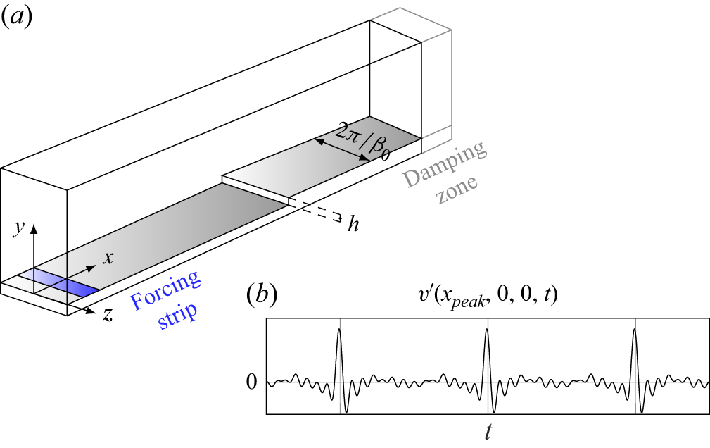
 xpeak

 x=0
 xst=0
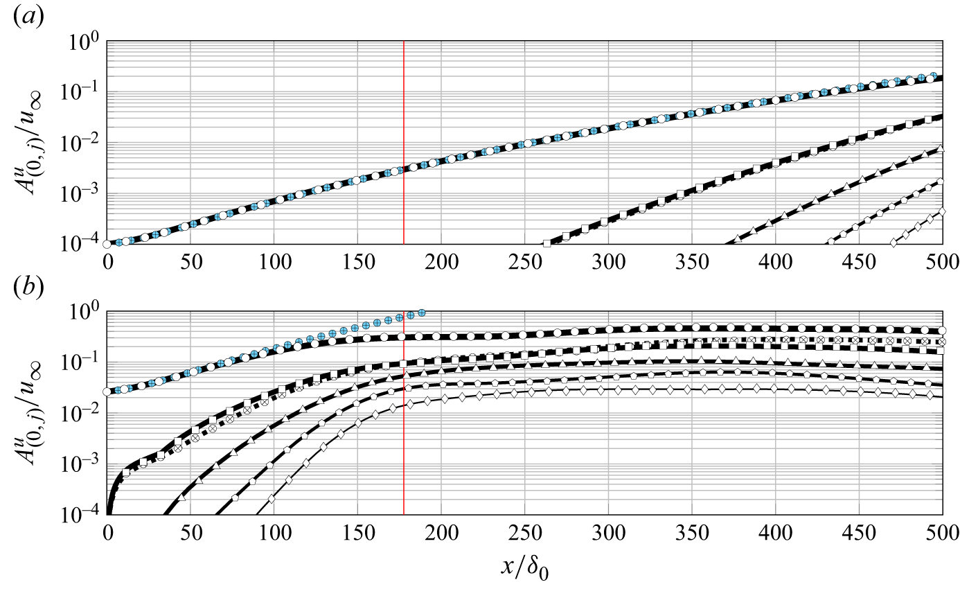
 j=1
 5
 j=0
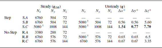
 Nx
 Ny
 Nz
 x
 y
 z
 Ny
 xst⩾0
 x
 z

 z
 y
 uDB,s
 xst/δ0=9.4
 wDB,s
 vDB

 ξw
 ∂uDB/∂y=0
 x
 z
 P/P0

 β=β0
 3β0

 y
 z
 ωxσB,(0,1)′
 v(0,1)′
 wσB,(0,1)′
 xst/δ0=0.3
 2.6
 7.6

 x
 Eint=∫Enβ0dy
 n=0
 1
 2
 3
 4
 5
 6
 (a,b)
 (e,f)
 (c,d)

 n=1

 n=3

 S
 n=0
 1
 2
 3
 4
 S

 S
 n=0
 1
 2
 3
 4
 S

 n=1
 uB=0

 n=3
 uB=0

 z
 y
 xst/δ0=9.4
 uDB,s⋆
 ⋆
 υB
 j
 uDB,s
 j=0,1
 j=0,3
 10

 170⩽x/δ0⩽184

 f=1
 8
 1

 Φ
 u∞δ0
 xst/δ0=5
 8
 10
 uDB,s
 0
 1.5u∞
 z⋆

 1
 12
 AM=∑j=−1313|u~|(k,j)2
 uDB=0
 z/δ0=−1.7
 z/δ0=4.8
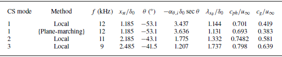
 maxx{−αθ,isecθ}
 N
 xst/δ0=10
 s=0.5δ0

 f=12
 u12′⋆=∑j=−1313u~(12,j)ei(jβ0z)/u∞+u~(−12,j)ei(jβ0z)/u∞
 xst/δ0≈5
 8
 10
 uDB/u∞
 0
 1.5u∞
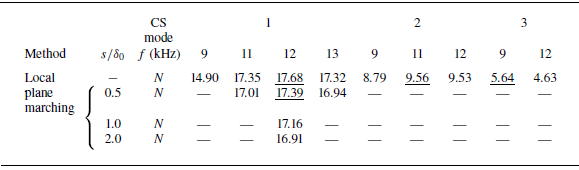
 N
 xst=10.38δ0
 x=188δ0

 |u~BiG|
 …
 maxz,y|u~BiG|
 xst/δ0
 maxx{−αθ,isecθ}
 xst/δ0=
 2.19
 2.49
 CS modes
 N
 xst/δ0=10
 uDB/u∞
 …

 a
 b
 CS-mode1
 s/δ0=0.5
 |u~BiG|
 1/8
 2/8
 …
 7/8
 maxz,y|u~BiG|
 CS-mode1
 12
 x
 s/δ0=0.5
 uDB/u∞
 10%
 20%
 …
 90%

 Q
 Qδ0/u∞=0.8
 x
 y
 y
 z
 z

 Q
 Qδ0/u∞=0.8
 z


 n=1
 n=3
 uB=0

 S
 n=0
 1
 2
 3

 a
 b
 c
 d
 z
 |u~|(12,j)
 CS-mode1
 |u~|(12,1)
 a
 xst/δ0=7.39

 αθ
 Δαθ
 αθ
 ω=2πf
 Δω/Δαθ∼cg→0
 αθ
 ω

 αθ,i
 αθ,r
 ωi
 αθ
 αθ,i→+∞

 Open access

