1. INTRODUCTION
Integrated navigation systems using a Global Navigation Satellite System (GNSS) receiver and an Inertial Navigation System (INS) based on a Micro-Electro-Mechanical System (MEMS) have been widely used due to advantages of low cost and miniaturisation (Abdel-Hafez et al., Reference Abdel-Hafez, Saadeddin and Jarrah2015; Cui et al., Reference Cui, Chen, Yuan, Huang and Xiao2017; Zhao et al., Reference Zhao, Qiu and Feng2016). However, GNSS signals may easily be blocked or lost when a vehicle is driving in complex environments, such as in forests and close to tall buildings (Elazab et al., Reference Elazab, Noureldin and Hassanein2017; Jaradat and Abdel-Hafez, Reference Jaradat and Abdel-Hafez2014), so that the GNSS/INS integrated navigation system works in pure INS mode. INS errors accumulate quickly with time due to MEMS-based inertial measurement units' bias error drift and scale factor instability (Liu et al., Reference Liu, Fan, Lv, Wu and Li2018), so a degradation of navigation performance is unavoidable during GNSS outages, and to improve accuracy, special approaches for correcting INS errors may need to be developed.
Relevant studies have developed a wide range of methods and modifications for improvement of GNSS/INS integrated systems. The existing approaches can be classified into two broad categories: one is based on Artificial Intelligence (AI), and the other is based on non-AI. The AI-based approaches include radial basis function neural networks (Sharaf and Noureldin, Reference Sharaf and Noureldin2007), adaptive neuro fuzzy inference system (Ahmed et al., Reference Ahmed, Khairulmizam and Abdul2011), hybrid Dempster-Shafer support vector machine (Bhatt et al., Reference Bhatt, Aggarwal, Devabhaktuni and Bhattacharya2014), genetic algorithm and support vector regression (Tan et al., Reference Tan, Wang, Jin and Meng2015), improved multi-layer perceptron (Yao et al., Reference Yao, Xu, Zhu and Chan2017), fuzzy inference system and sparse random Gaussian (Havyarimana et al., Reference Havyarimana, Hanyurwimfura, Nsengiyumva and Zhu2018). Basically, the AI is trained to model the relationship of INS outputs and INS errors when GNSS signals are available. In the case of outages, the trained mode is utilised to predict and compensate for the INS errors. However, these AI-based methods demand a great deal of training data and relatively long training periods for robust generalisation. Moreover, the high bias instability and scale factor of MEMS-based inertial sensors increase the nonlinear complexity of the input/output functional relationship and limit the AI generalisation ability that in turn affects its prediction accuracy.
Some studies have suggested incorporation of appropriate constraints such as zero lateral and vertical velocities (Nassar et al., Reference Nassar, Syed, Niu and El-Sheimy2006) and zero short-term height variations (Godha and Cannon, Reference Godha and Cannon2007). In addition, some auxiliary sensors such as odometer, Doppler velocity log and vision machine can be implemented on the system to provide external observations during GNSS outages (Brown and Lu, Reference Brown and Lu2004; Aftatah et al., Reference Aftatah, Lahrech and Abounada2017), but these will increase the cost and complexity of the integrated system. In addition, some modifications to a Kalman Filter (KF) can also enhance the performance of the integrated system. Nevertheless, even an improved KF works for a short time in prediction mode due to GNSS outages; the overall performance of GNSS/INS based on MEMS will be degraded (Quinchia et al., Reference Quinchia, Falco and Falletti2013). To overcome the weaknesses related to the AI-based methods and the above non-AI methods, the Auto-Regressive Forward Estimator (ARFE) and Grey Predictor (GP) have been designed to predict and compensate INS position errors during GNSS outages (Chen et al., Reference Chen, Li, Song, Li, Song and Xu2015; Li and Xu, Reference Li and Xu2017). The ARFE method needs to solve at least three parameters, while the GP model only needs to calculate two parameters. The ARFE and GP have the advantages of low computational burden and good real-time performance, but their ability to deal with nonlinear problems is weak, so the prediction accuracy is limited.
In order to integrate the advantages of AI-based methods and non-AI methods, a novel hybrid algorithm utilising grey system theory and artificial neural network is proposed. Grey system theory is an interdisciplinary scientific area that was introduced in 1980s by Deng (Deng, Reference Deng1982; Reference Deng1989) and has been used to compensate for GNSS location fault data (Zhou and Zhang, Reference Zhou and Zhang2010; Wang et al., Reference Wang, Che, Lu and Gao2015; Venkateswarlu and Sarma, Reference Venkateswarlu and Sarma2017). However, the prediction accuracy is often low (Kayacan et al., Reference Kayacan, Ulutas and Kaynak2010). The discrete grey forecasting model was proposed to improve the predicting performance of the grey predictor (Xie and Liu, Reference Xie and Liu2009). The Discrete Grey Predictor (DGP) is constructed for both estimating parameters and simulating and forecasting values with discrete equations, which overcomes the GP's problem when it skips from the discrete equation to the continuous equation. The Multilayer Perceptron (MLP) neural network is improved by adding momentum terms, adaptively adjusting the learning rate and momentum factors. The proposed DGP-MLP algorithm not only has the advantages of the discrete grey predictor aimed at an uncertain system and less data, but also has the characteristics of a neural network to deal with nonlinear problems. The DGP-MLP can predict the pseudo-GNSS position information by using the latest few moments' data effectively and improve the integrated navigation performance during GNSS outages.
The structure of this paper is as follows: Section 2 gives a brief overview of a GNSS/INS loosely-coupled integrated system. In Section 3, the discrete grey predictor and the improved multilayer perceptron neural network are presented. An integration scheme operating during GNSS outages and the implementation of DGP-MLP are researched in detail. In Section 4, road experiments that validate the proposed algorithm are presented and discussed. Section 5 concludes the paper.
2. GNSS/INS LOOSELY-COUPLED INTEGRATED SYSTEM
Here, the GNSS/INS integrated navigation system adopts a loose combination mode. The estimated values of position are obtained by GNSS and INS, then the corresponding differences can be obtained, and they are input into the KF. The outputs of the filter, which are called estimated errors, are fed back to the INS and used to correct the INS outputs. In this way, the INS outputs become more accurate.
2.1. INS error model
According to the measured specific forces and angular increments of INS, the navigation information (position, velocity and attitude) can be solved. The navigation frame adopts an East-North-Upward (ENU) geographic coordinate system and the body frame adopts a Right-Forward-Up (RFU) coordinate system. The detailed derivation process of INS error equations can be found in Titterton and Weston (Reference Titterton and Weston2004) and Liu et al. (Reference Liu, Fan, Lv, Wu and Li2018).
The attitude error of an INS can be described as follows:
 $${\bi \dot{\psi }}^n = \delta {\bi \omega }_{ie}^n + \delta {\bi \omega }_{en}^n -({\bi \omega }_{ie}^n + {\bi \omega }_{en}^n ) \times {\bi \psi }^n-{\bi \varepsilon }^n$$
where ψn = [ψ E, ψ N, ψ U] T is the attitude angle error vector in the ENU frame, ψE is the pitch angle error, ψN is the roll angle error and ψU is the yaw angle error.  ${\bf {\omega}}_{ie}^{n}$ and
 $\delta {\bf {\omega}}_{ie}^{n}$ are the rotating angular velocity and its error caused by the Earth's rotation, respectively.
 ${\bf {\omega}}_{en}^{n}$ and
 $\delta {\bf {\omega}}_{en}^{n}$ represent the angular velocity of the rotation of a navigation coordinate frame relative to Earth and its error. εn is the gyroscope drift vector in the navigation coordinate frame.
The INS velocity error equation is given by:
 $$\delta \dot{V}^n = f^n \times \psi ^n-(2\delta \omega _{ie}^n + \delta \omega _{en}^n ) \times V^n-(2\omega _{ie}^n + \omega _{en}^n ) \times \delta V^n + \nabla ^n$$
where δ Vn = [δV E, δV N, δV U] T is the velocity error vector, δ V E is the east velocity error, δ V N is the north velocity error and δ VU is the upward velocity error. Vn = [V E, V N, V U] T denotes the velocity vector, VE is the east velocity, V N is the north velocity and V U is the upward velocity. fn is the specific force vector, and  ${\bf {\nabla}}^{n}$ is the biases of the accelerometer in the navigation frame.
The position error equations can be expressed as:
 $$\left\{ {\matrix{ {\delta \dot{L} = \displaystyle{1 \over {R_N + h}}\delta V_N-\displaystyle{{V_N} \over {{(R_N + h)}^2}}\delta h} \cr {\delta \dot{\lambda } = \displaystyle{{\sec L} \over {R_E + h}}\delta V_E + \displaystyle{{V_E} \over {R_E + h}}\sec L\cdot \tan L\cdot \delta L-\displaystyle{{V_E\sec L} \over {{(R_N + h)}^2}}\delta h} \cr {\delta \dot{h} = \delta V_U} \cr } } \right.$$
where L, λ and h are latitude, longitude and height, respectively. δ L, δλ and δ h are latitude, longitude and height errors, respectively. R E and R N are the radii of the curvatures along the meridian and the radii of the curvatures along the parallel to the equator.
2.2. Kalman Filter (KF)
A KF is an optimal estimation, which has good real-time performance and simple operation, and has been widely used in integrated navigation systems (Yao et al., Reference Yao, Xu, Zhu and Chan2017; Sang and Hwang, Reference Sang and Hwang2017). Although a KF is mainly applied to linear systems, it can still achieve good performance due to the low nonlinearity of the integrated navigation system.
Considering the system precision and real-time, the fifteen-dimensional state vector includes three attitude errors, three velocity errors, three position errors, three accelerometer biases and three gyroscope drifts. The state vector X can be expressed as:
 $${\bi X} = \lsqb {\psi_E,\psi_N,\psi_U,\delta V_E,\delta V_N,\delta V_U,\delta L,\delta \lambda ,\delta h,\nabla_{bx},\nabla_{by},\nabla_{bz},\varepsilon_{bx},\varepsilon_{by},\varepsilon_{bz}} \rsqb ^T$$
where ∇bx, ∇by and ∇bz denote three accelerometer biases. εbx, εby and εbz denote three gyro drifts, respectively.
The KF uses a perturbation error model of the inertial navigation system. Based on the error model in Equations (1)–(3), the discrete state equation and the measurement equation are as follows:
 $$\left\{ {\matrix{ {{\bi X}_k = {\bi F}_{k,k-1}{\bi X}_{k-1} + {\bi G}_k{\bi W}_k} \cr {{\bi Z}_k = {\bi H}_k{\bi X}_k + {\bi V}_k} \cr } } \right.$$
where Fk,k−1 is the system state transition matrix, Gk is the system noise distribution matrix, Wk and Vk are process and measurement noise, Hk represents the measurement matrix and Zk is the measurement vector.
The KF consists of a time prediction and a measurement update. The time prediction equations are responsible for the forward time transition from the epoch k − 1 state to the next epoch k state. The time prediction equations are given by:
 $$\hat{\bi X}_{k,k-1} = {\bi F}_{k,k-1} {\bi X}_{k-1}$$
 $${\bi P}_{k,k-1} = {\bi F}_{k,k-1} {\bi P}_{k-1} {\bi F}_{k,k-1}^T + {\bi Q}_{k-1}$$
where  $\hat{\bi X}_{k\comma k-1}$ is the a priori estimate value of the state vector, Pk,k−1 is the a priori estimate error covariance matrix, Pk−1 is the a posteriori estimate error covariance matrix and Qk−1 is the process noise covariance matrix.
The measurement update equations are given by:
 $${\bi K}_k = {\bi P}_{k,k-1}{\bi H}_k^T \left[ {{\bi H}_k{\bi P}_{k,k-1}{\bi H}_k^T + {\bi R}_k} \right]^{-1}$$
 $$\hat{\bi {X}}_k =\hat{\bi {X}}_{k,k-1} + {\bi {K}}_k \lpar {{Z}_k - {\bi {H}}_k \hat{\bi {X}}_{k,k-1} }\rpar $$
 $${\bi {P}}_k ={\bi {P}}_{k,k-1} - {\bi {K}}_k {\bi {H}}_k^T {\bi {P}}_{k,k-1}$$
where Kk is the Kalman gain matrix,  $\hat{\bi {X}}_{k}$ is the a posteriori estimated value of the state vector, and Rk is the measurement error covariance matrix. A detailed introduction to KFs can be found in Julier and Uhlmann (Reference Julier and Uhlmann1997).
3. HYBRID INTELLIGENT ALGORITHM DGP-MLP
Grey system theory requires fewer samples, simple model construction and less computation, but it lacks self-learning and self-adaptive ability. The artificial neural network has good nonlinear fitting and self-adaptive ability but requires a large number of training samples. By using the hybrid intelligent algorithm, the DGP-MLP has the advantages of grey system theory and artificial neural networks.
3.1. Discrete grey predictor
Since grey system theory was first introduced, the grey forecasting model has been widely adopted. However, the precision of the GP model may sometimes be unsatisfactory. In the GP model, the method of estimating parameters is the discrete equation and the method of simulating and forecasting is the continuous equation. The different forms of the discrete equation and the continuous equation will produce different estimated results. So, the skip from the discrete equation to the continuous equation is the problem which caused the error in simulation and forecasting. The DGP model is constructed for both estimating parameters and simulating and forecasting values with discrete equations. The DGP (1, 1) is established, and the modelling steps are as follows (Xie and Liu, Reference Xie and Liu2009).
3.1.1. Data pre-processing
If there are negative numbers in the original data, the modelling condition (sequence level judgment) of DGP cannot be satisfied. Usually, a constant can be added to the original data, and the original sequence is transformed into the non-negative sequence. The sequence can be given as:
 $${\bi {X}}^{(0)}=\lcub {x^{(0)}(1),x^{(0)}(2),\cdots ,x^{(0)}(i),\cdots ,x^{(0)}(n)} \rcub $$
where X(0) is the input data of the DGP model, x (0)(i) is the i-th element and n is the length of the input vector. When using different lengths of original data for modelling, the predicted value for the same time will be different, so the value of n will affect the prediction accuracy. The choice of the best value is dependent on the sensor data and this can be performed during offline analysis.
3.1.2. Accumulated generating operation
Taking the accumulated generating operation on X(0), the accumulated sequence X(1) can be obtained as:
 $${\bi {X}}^{(1)}=\lcub {x^{(1)}(1),x^{(1)}(2),\cdots ,x^{(1)}(k),\cdots ,x^{(1)}(n)} \rcub $$
where X(1) is the accumulated sequence of input data. x (1)(k) is the k-th element,  $x^{{\rm (}1{\rm )}}{\rm (}k{\rm )} = \sum\nolimits_{i = 1}^k {x^{{\rm (}0{\rm )}}{\rm (}i{\rm )}} $, k = 1, 2,···, n.
3.1.3. Establish DGP (1, 1)
The DGP (1, 1) model is established as:
 $$\hat{x}^{(1)}(l+1)=U_1 \hat{x}^{(1)}(l)+U_2$$
where U 1 and U 2 are the development coefficients,  $\hat{x}^{\lpar 1\rpar }\lpar l\rpar $ is the l-th predicted value of the accumulated data, l = 1, 2, · · · , n, · · · , n + m, m is the length of the prediction sequence and can be determined according to the length of the assumed GNSS outage. The precision of the DGP model will decrease with the increase of m, so the DGP is usually used in predicting the short-term developing trend of a data sequence.
To solve Equation (13), the coefficients U 1 and U 2 must be determined. They can be solved by means of the least squares method as follows:
 $$\hat{{\bi {U}}}=({\bi {B}}^T {\bi {B}})^{-1} {\bi {B}}^T {\bi {Y}}$$
where  $\hat{{\bi U}} = \left[{\matrix{ {U_1} \cr {U_2} \cr } } \right]\comma \; {\bi Y} = \left[{\matrix{ {x^{\lpar 1\rpar }\lpar 2\rpar } \cr {x^{\lpar 1\rpar }\lpar 3\rpar } \cr \vdots \cr {x^{\lpar 1\rpar }\lpar n\rpar } \cr } } \right]\comma \; {\bi B} = \left[{\matrix{ {x^{\lpar 1\rpar }\lpar 1\rpar } & 1 \cr {x^{\lpar 1\rpar }\lpar 2\rpar } & 1 \cr \vdots & \vdots \cr {x^{\lpar 1\rpar }\lpar n-1\rpar } & 1 \cr } } \right]$.
Set  $\hat{x}^{\lpar 1\rpar }\lpar 1\rpar =x^{\lpar 1\rpar }\lpar 1\rpar $, then predicted value of the accumulated data
 $\hat{x}^{\lpar 1\rpar }\lpar {l+1}\rpar $ can be obtained as:
 $$\hat{x}^{(1)}(l + 1) = U_1^l \hat{x}^{(1)}(1) + \displaystyle{{1-U_1^l } \over {1-U_1}}U_2$$
3.1.4. Inverse accumulated generating operation
Note that the DGP (1, 1) model designed above is updated when GNSS works normally. Once GNSS fails, the latest DGP (1, 1) model is utilised to predict the corresponding position, which can be calculated by the inverse accumulated generating operation on x̂ (1) (Xie and Liu, Reference Xie and Liu2009). The estimated value x̂ (0) can be given by:
 $$\hat{x}^{(0)}(l+1)=\hat{x}^{(1)}(l+1)-\hat{x}^{(1)}(l)$$
The grey prediction value is the estimated value after post-processing.
3.2. Improved multilayer perceptron
The multilayer feed-forward neural network is a common and effective machine learning method for nonlinear function fitting. This type is commonly referred to as MLP, whose structure mainly consists of one input layer, one or more hidden layers, and one output layer. The nodes of each layer are connected with weights, and the nodes of hidden layers consist of nonlinear or linear activation functions.
The relationship between input and output of the MLP can be expressed as follows:
 $${\bi a}_O = f_2\left( {{\bi \omega }_O*{f}_{\rm 1}\left( {{\bi \omega }_H*{\bi a}_I + {\bi b}_H} \right) + {\bi b}_O} \right)$$
where aI is the input vector and aO is the output vector. f 1 and f 2 are the transfer functions of the hidden layer and the output layer, respectively. ωH and ωO are the weight matrices of the hidden layer and the output layer, respectively. The bias terms are also added to the neurons in the hidden layer and the output layer, grouped into bH and bO, respectively.
Error reverse correction is realised by updating the parameters to minimise the object loss function with a gradient descent algorithm until the loss function converges. The hidden layer parameters are updated by:
 $$\eqalign{& {\bi \omega }_{H,t + 1} = {\bi \omega }_{H,t}-\alpha \displaystyle{{\partial E_t} \over {\partial {\bi \omega }_{H,t}}} \cr & {\bi b}_{H,t + 1} = {\bi b}_{H,t}-\alpha \displaystyle{{\partial E_t} \over {\partial {\bi b}_{H,t}}}}$$
where E is the mean squared error loss between aO and the actual value, α is the learning rate and t is the index of t-th update. ωO,t+1 and bO,t+1 can be obtained in the same way.
The MLP is a nonlinear model, which has the ability to estimate complicated functions. However, this ability makes it vulnerable to over-fit the training data and to get stuck in the local optimum (Srivastava et al., Reference Srivastava, Hinton, Krizhevsky, Sutskever and Salakhutdinov2014), and the convergence rate is slow. To overcome these deficiencies, based on the improved MLP with additional momentum terms and an adaptive learning factor, the additional momentum factor is made to be self-adaptive for further optimisation and improvement.
3.2.1. Adding momentum terms
The momentum terms are added to suppress falling into the local optimum. The additional momentum terms are based on the last moment parameter. The hidden layer parameters are expressed as:
 $$\eqalign{& {\bi \omega }_{H,t + 1} = {\bi \omega }_{H,t}-\alpha \displaystyle{{\partial E_t} \over {\partial {\bi \omega }_{H,t}}}-\eta {\bi \omega }_{H,t-1} \cr & {\bi b}_{H,t + 1} = {\bi b}_{H,t}-\alpha \displaystyle{{\partial E_t} \over {\partial {\bi b}_{H,t}}}-\eta {\bi b}_{H,t-1}}$$
where η is the momentum factor, and the value is usually between 0 and 1. ωO,t+1 and bO,t+1 can be obtained in the same way.
When the gradient keeps pointing in the same direction, this will increase the steps taken towards the minimum. On the other hand, momentum will smooth out the variations when the gradient keeps changing direction.
3.2.2. Adaptive learning rate α and momentum factor η
In the MLP algorithm, the learning rate α is critical. If α is large, the MLP converges quickly, but may cause oscillation. While a small value can avoid oscillation, the convergence speed is slow. The initial value of the momentum factor η also has great impact on the convergence rate. An adaptive learning rate and momentum factor can improve convergence performance. The adaptive law of learning rate α and momentum factor η can be designed as:
 $$\eqalign{& \Delta p_t = \left\{ {\matrix{ {a\cdot p_{t-1}} \hfill & {E_t\downarrow } \hfill \cr {-b\cdot p_{t-1}} \hfill & {E_t\uparrow } \hfill \cr 0 \hfill & {else} \hfill \cr } } \right. \cr & p_t^{\prime} = p_t + \Delta p_t}$$
where a and b are adaptive factors and are set to 0 to 1. In the following experiments, they were set to 0.2. p represents α or η. If the error becomes smaller, indicating the current direction is correct, then p will be increased; in contrast, if the current direction is not correct, then p is appropriately reduced.
3.3. DGP-MLP aided GNSS/INS integrated system scheme
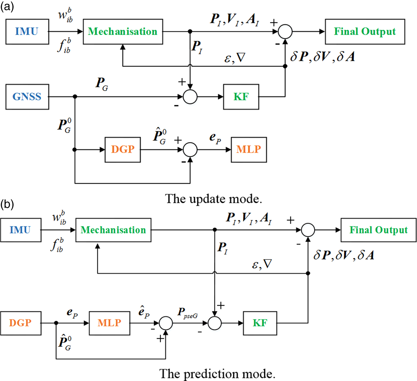
To achieve accurate and reliable positioning performance, a hybrid intelligent methodology that combines the advantages of DGP and MLP techniques is proposed. The structure of our DGP-MLP-aided GNSS/INS integrated system is shown in Figure 1.
DGP-MLP aided GNSS/INS integrated system structure.

When GNSS signals are available, the system operates in the update (that is, training) mode, as shown in Figure 1(a). P, V and A are position, velocity and attitude, respectively and δ indicates error. The outputs of the INS and GNSS are integrated by the KF, where the attitude, velocity, and position errors are estimated as a correction to the INS outputs. Meanwhile, the GNSS position  ${\bi {P}}_{G}^{0}$ is sent to the DGP model as the input, and the predicted position
 $\hat{\bi {P}}_{G}^{0}$ is the output of the DGP. The residual eP is used to train the MLP model.
Whenever the GNSS signals are unavailable, the system operation automatically switches to the prediction mode shown in Figure 1(b). In this case, the residual eP is provided as the input of MLP, and the output of MLP is the predicted residual  $\hat{\bi {e}}_{P} $. The relationship between eP and
 $\hat{\bi {e}}_{P}$ is nonlinear, which can be well handled by MLP. After the integral, the pseudo-GNSS position information PpseG can be achieved, which is then used as the input of the KF to form the observation vector with the INS position. The navigation system will continuously give integrated information during GNSS outages.
The procedure of the proposed DGP-MLP method is as follows:
3.3.1. DGP prediction
The original GNSS position is expressed as  $\lcub {P_{G}^{0} \lpar i\rpar } \rcub $, i = 1, 2,···, n. The prediction value
 $\lcub {\hat{P}_{G}^{0} \lpar j\rpar } \rcub $, j = 1, 2, · · · , n + m can be obtained by DGP.
3.3.2. Establish MLP training model of residual sequence
The residual at time k is defined as e P (k), that is  $e_{P} \lpar k\rpar =\hat{P}_{G}^{0} \lpar k\rpar -P_{G}^{0} \lpar k\rpar $, k = 1, 2,···, n. Let S be the prediction order, and l 1 is an index value for building an input/output vector of the MLP training mode. The input vector of the MLP training mode is e P(l 1 − 1), e P(l 1 − 2), · · · , e P(l 1 − S). The output of the MLP training model is e P (l 1), l 1 = S + 1, S + 2, · · · , n. The prediction order S affects the structure of the MLP, including the numbers of input layer nodes and hidden layer nodes, and thus affects the estimation accuracy. In order to reach a balance between efficiency, real-time operation and effectiveness, S is set to 4.
3.3.3. Predicted value modified by residual
The input of the MLP prediction mode is e P(l 2 − 1), e P(l 2 − 2), · · · , e P(l 2 − S), and the output of the MLP prediction mode is the predicted residual  $\hat{e}_{P} \lpar l_{2}\rpar $, where l 2 is an index value for building an input/output vector of the MLP prediction mode, l 2 = n + 1, n + 2, · · · n + m. The predicted residual is used to compensate
 $\hat{{\bi {P}}}_{G}^{0}$, then the corrected prediction can be obtained
 $P_{pseG} \lpar l_{2}\rpar =\hat{P}_{G}^{0} \lpar l_{2}\rpar -\hat{e}_{P} \lpar l_{2}\rpar $.
4. EXPERIMENTAL RESULTS
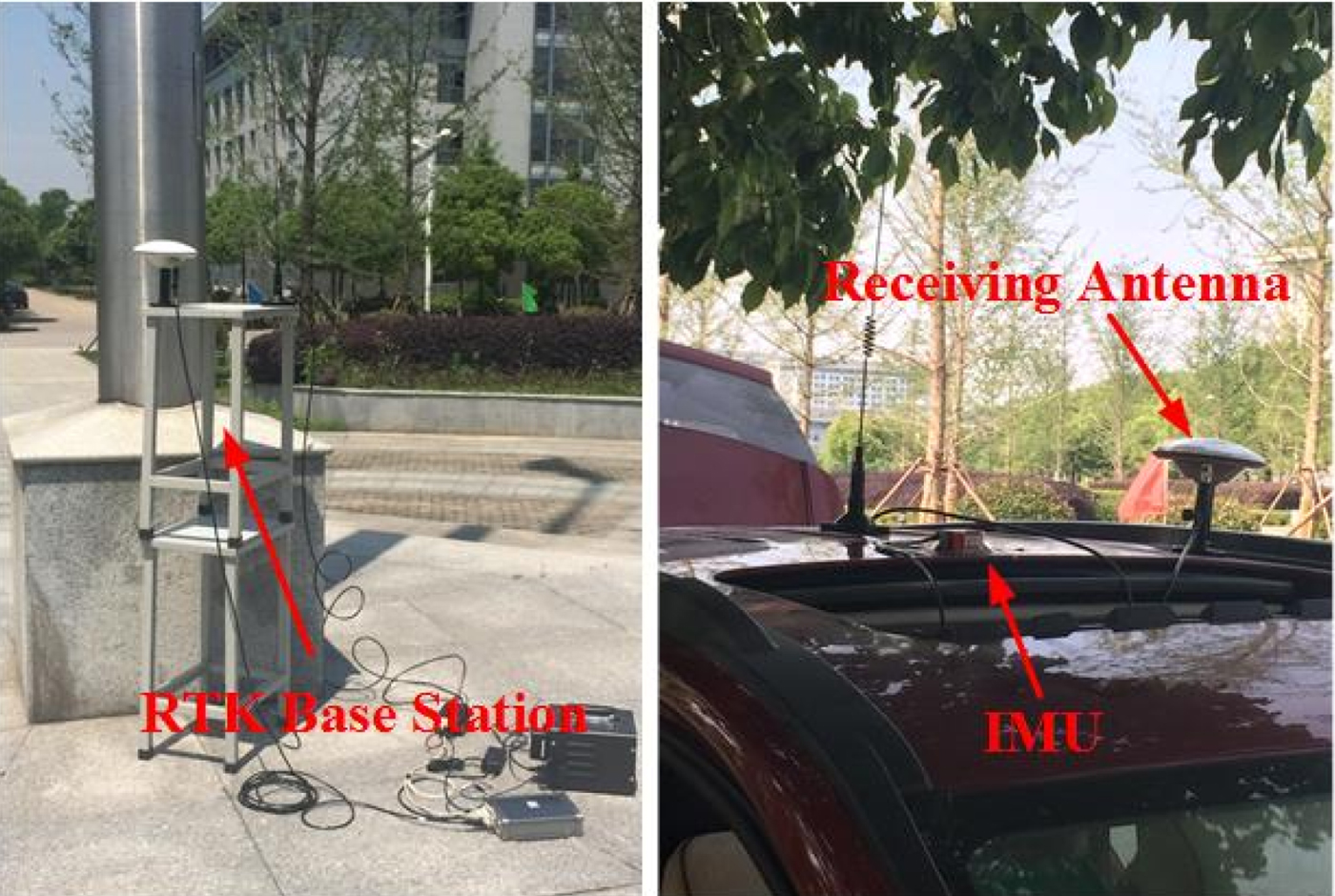
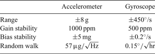
To evaluate the positioning performance of the proposed algorithm, experiments were conducted in the Jiulonghu campus of Southeast University, Nanjing, Jiangsu Province, China. A MEMS-based Inertial Measurement Unit (IMU) utilising the Ellipse-A IMU of SBG Systems sampled at 100 Hz was installed. Real-Time Kinematic (RTK) GNSS can provide high precision navigation, and its results combined with INS can be taken as the positioning reference or the “real” trajectory. The RTK base station sends the received satellite signals to the receiver, and the receiver (a TRIMBLE BD982 GNSS receiver outputting at 1 Hz) calculates the coordinates according to the received satellite signals and the base station signals. Thus, in actual implementation, the rate of INS calculation is set as 100 Hz whereas the DGP-MLP algorithm works at 1 Hz. The specifications and main parameters of the MEMS-based IMU can be found in Table 1. The test vehicle with navigation system equipment are shown in Figure 2.
Test vehicle with navigation system equipment.

Characteristics of Ellipse-A IMU.

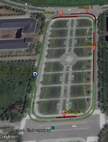
Figure 3 shows the field test trajectory. After all sensor data were collected, four simulated GNSS outages were intentionally introduced within the trajectory by artificially removing the GNSS solution in order to assess the performance of the proposed method. The selected GNSS outages route included typical conditions such as south-north movement, east-west movement and turning, as shown in Figure 3, where the green line represents the field test trajectory and the red line indicates the simulated GNSS outages.
Experimental trajectory with four simulated GNSS outages.

The proposed DGP-MLP method is based on DGP and uses MLP to correct DGP residuals. To highlight the advantages of the proposed method, four other methods were also investigated. 1) The pure INS method (Pure INS). This only fuses the information of GNSS and MEMS-based IMU through the common KF. When the GNSS signal is lost, the system works in purely INS mode. 2) The Grey Predictor method (GP): This uses the common grey prediction theory to provide pseudo-GNSS position during GNSS outages. 3) The Discrete Grey Predictor method (DGP): Compared with the GP method above, it improves the limitations of the GP method by using a discrete form. However, it does not utilise the MLP to correct residuals. 4) The Auto-Regressive Forward Estimator (ARFE): A hybrid strategy incorporating the ARFE with a Kalman filter is used to compensate the INS position errors during GNSS outages (Chen et al., Reference Chen, Li, Song, Li, Song and Xu2015).
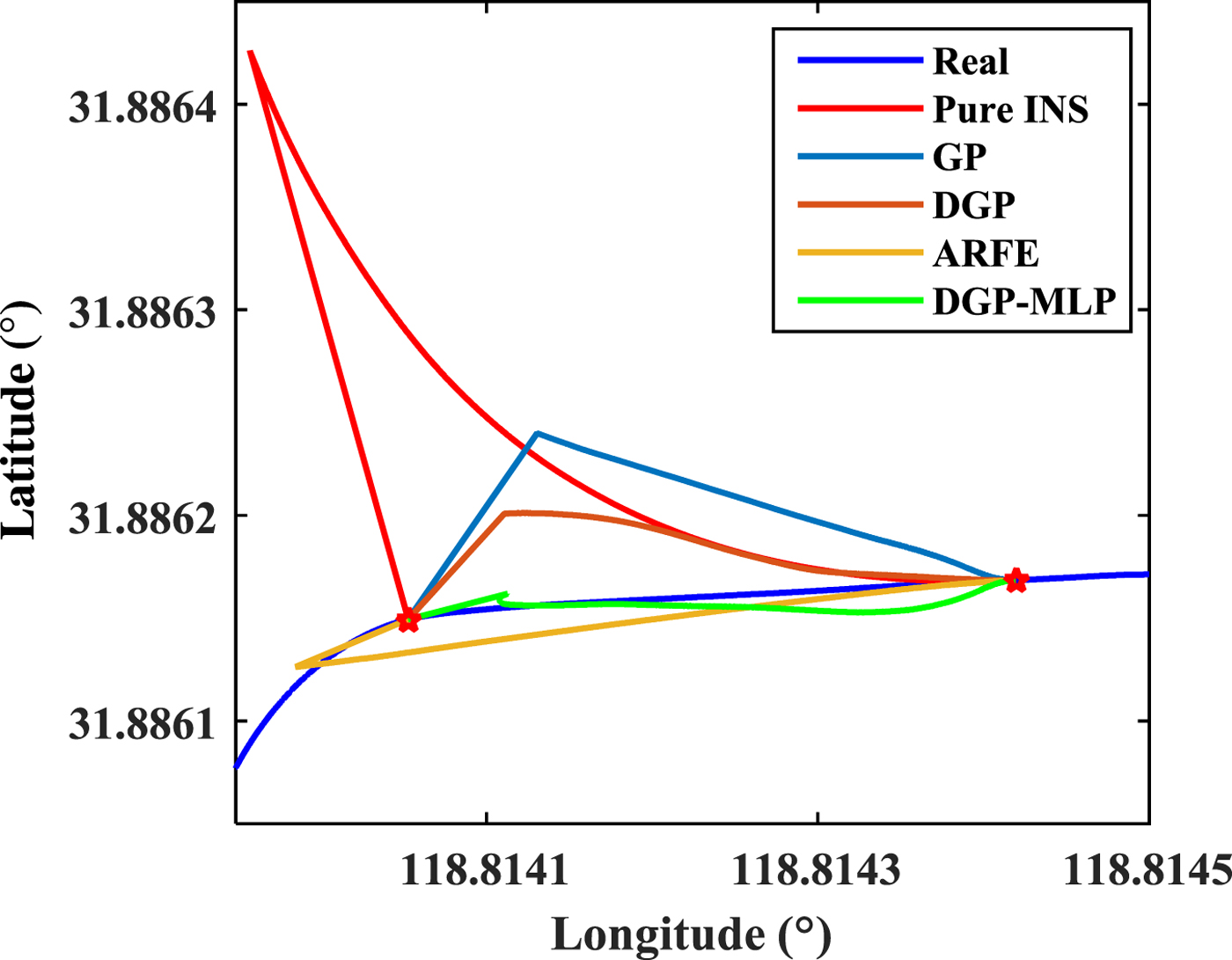
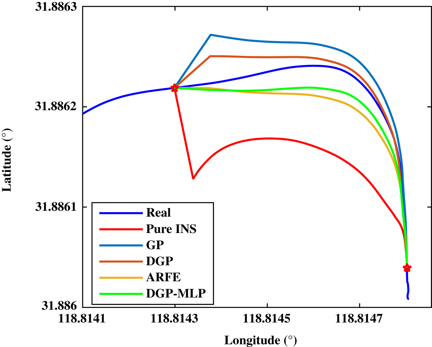
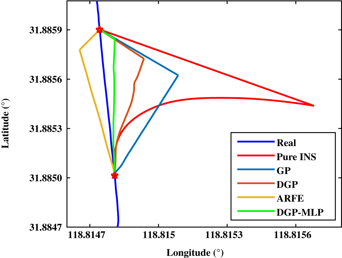
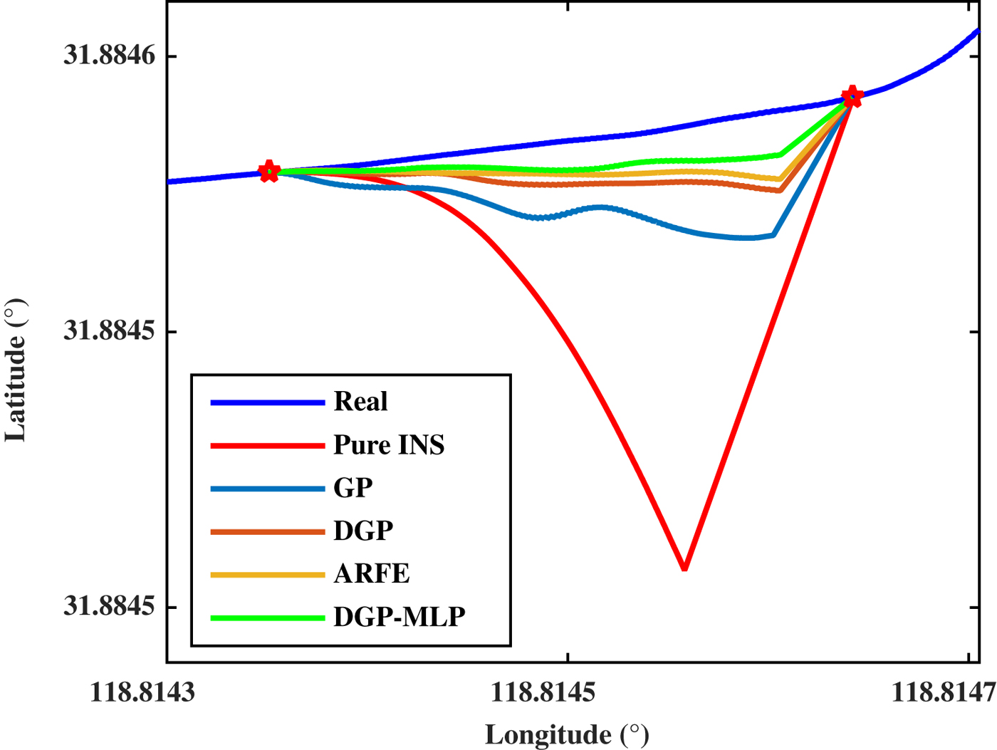
For the positioning methods above, Tables 2 and 3 give the maximum and Root Mean Square (RMS) values of horizontal position errors during four GNSS outages, respectively. Figures 4–7 give the positioning results.
Positioning results during GNSS outage 1 (the red five-point stars in Figures 4–7 denote the beginning/end positions of GNSS outages).

Positioning results during GNSS outage 2.

Positioning results during GNSS outage 3.

Positioning results during GNSS outage 4.

Maximum position errors during GNSS outages (Unit: m).

RMS position errors during GNSS outages (Unit: m).

From Tables 2–3 and Figures 4–7, the five methods exhibit remarkably different positioning performance during GNSS outages.
The pure INS method has the worst positioning performance. For each outage, both the maximum and RMS values of its position error are the largest, and cannot meet the positioning requirements. For example, the maximum and RMS errors for outage 3 reach 104.37 m and 32.44 m, respectively. This can be attributed to fact that this method simply integrates GNSS with a low-cost MEMS-based IMU, which cannot ensure positioning accuracy and reliability during the period of GNSS outage.
The GP method can achieve a better performance than the pure INS in all situations. For instance, for outage 3, the maximum and RMS values of position error of GP method are reduced to 38.19 m and 20.38 m, respectively. These results verify the effectiveness of the model in Figure 1, and a pseudo-GNSS position is available. However, the grey predictor still needs to be improved since its accuracy is limited.
For the DGP method, the positioning accuracy is improved compared with that of the GP method during the four GNSS outages. The DGP method can maintain maximum position errors within the range of 3–22 m (the RMS range is 1–12 m), as opposed to the range of 4–39 m (the RMS range is 1–21 m) achieved by the GP method. For the four GNSS outages, the average improvements are 21.73% and 26.33% for the maximum and RMS errors, respectively. The reason that the DGP has better prediction precision is that the DGP improves the traditional GP by adopting discrete methods.
Among the five methods, the proposed method (that is, DGP-MLP) achieves the best accuracy and reliability. Compared with the DGP method, the proposed method still provides significant performance improvement. The range of maximum position error of the proposed method is reduced to 3–8 m from the range 3–22 m of the DGP method, which achieves 19.02% average performance improvement. In addition, the range of RMS position error of the proposed method is within 1–4 m in comparison with the RMS range 1–12 m for the DGP method; that is a 34.16% average accuracy enhancement. To prove the benefit of the proposed method, the DGP-MLP is also compared with a conventional method ARFE. In Chen et al. (Reference Chen, Li, Song, Li, Song and Xu2015), the AR model is fourth order, and can get better predicted results and guarantee efficiency. So, the ARFE method needs to solve four parameters, while the DGP model only needs to calculate two parameters. In addition, a digital compass is adopted by Chen et al. to improve position accuracy, which increases the cost and structure complexity. Moreover, the experimental results show that the DGP-MLP has better performance than ARFE. For four GNSS outages, the average improvements are 16.15% and 26.83% for the maximum and RMS errors, respectively.
5. CONCLUSIONS
A novel hybrid fusion methodology DGP-MLP has been proposed to improve the performance of a low-cost GNSS/INS integration system during GNSS outages. This hybrid approach aggregates the advantages of both a discrete grey predictor and artificial neural network, leading to a substantial decrease in positional drift and positioning error. The DGP predicts GNSS position and MLP captures the non-linearity left in the residuals that DGP could not capture. Compared with DGP, DGP-MLP improves the average of maximum errors and the average of RMS errors by 19.02% and 34.16%, respectively. Thus, the results obtained demonstrate the potential of the DGP-MLP model during GNSS outages effectively, thereby making the navigation continuous and reliable. Future work will concern how to enhance the navigation performance over longer GNSS outage conditions and in real-time application.
FINANCIAL SUPPORT
The project was supported by following funds: National Key Research and Development Program (2016YFD0702000), National Natural Science Foundation of China (61773113, 41704025), Natural Science Foundation of Jiangsu Province (BK20160668).