2.1 The CCS and non-conservative PCS models

The standard PCS appearing in the literature (Cheng Reference Cheng1991; Park et al. Reference Park, Parker, Biglari, Chance, Chen, Cheng, Hahm, Lee, Kulsrud and Monticello1992; Fu & Park Reference Fu and Park1995; Kim et al. Reference Kim, Sovinec and Parker2004) can be easily formulated starting from the following equations for the CCS (Belova & Park Reference Belova, Park, Yoshimura and Seiichi1999; Belova et al. Reference Belova, Gorelenkov, Fredrickson, Tritz and Crocker2015), which serve as our point of departure in this discussion:

(2.1) $$\begin{eqnarray}\displaystyle & \displaystyle \unicode[STIX]{x1D70C}\unicode[STIX]{x2202}_{t}\boldsymbol{u}+\unicode[STIX]{x1D70C}(\boldsymbol{u}\boldsymbol{\cdot }\unicode[STIX]{x1D735})\boldsymbol{u}=(q_{h}n_{h}\boldsymbol{u}-a_{h}\boldsymbol{K}_{h}+\boldsymbol{J})\times \boldsymbol{B}-\unicode[STIX]{x1D735}\mathsf{p}, & \displaystyle\end{eqnarray}$$

(2.2) $$\begin{eqnarray}\displaystyle & \displaystyle \unicode[STIX]{x2202}_{t}\unicode[STIX]{x1D70C}+\unicode[STIX]{x1D735}\boldsymbol{\cdot }(\unicode[STIX]{x1D70C}\boldsymbol{u})=0, & \displaystyle\end{eqnarray}$$

(2.3) $$\begin{eqnarray}\displaystyle & \displaystyle \unicode[STIX]{x2202}_{t}f+\boldsymbol{v}\boldsymbol{\cdot }\unicode[STIX]{x1D735}f+a_{h}(\boldsymbol{v}-\boldsymbol{u})\times \boldsymbol{B}\boldsymbol{\cdot }\frac{\unicode[STIX]{x2202}f}{\unicode[STIX]{x2202}\boldsymbol{v}}=0, & \displaystyle\end{eqnarray}$$

(2.4) $$\begin{eqnarray}\displaystyle & \displaystyle \unicode[STIX]{x2202}_{t}\boldsymbol{B}=\unicode[STIX]{x1D735}\times (\boldsymbol{u}\times \boldsymbol{B}). & \displaystyle\end{eqnarray}$$

Here $\boldsymbol{u}$ is the bulk fluid velocity, $\boldsymbol{J}=\unicode[STIX]{x1D707}_{0}^{-1}\unicode[STIX]{x1D735}\times \boldsymbol{B}$ is the usual MHD current, $q_{h}$ and $m_{h}$ are the charge and the mass of the energetic particles respectively and $a_{h}=q_{h}/m_{h}$ . In addition, the energetic particle density on phase space, $f(\boldsymbol{x},\boldsymbol{v})$ , generates the following moments

(2.5) $$\begin{eqnarray}\displaystyle n_{h}=\int f\,\text{d}^{3}v,\quad \boldsymbol{K}_{h}=m_{h}\int \boldsymbol{v}f\,\text{d}^{3}v. & & \displaystyle\end{eqnarray}$$

The interested reader can find the detailed derivation of the equations (2.1)–(2.4) in both the original work (Park et al. Reference Park, Parker, Biglari, Chance, Chen, Cheng, Hahm, Lee, Kulsrud and Monticello1992) as well as in more recent papers (Tronci et al. Reference Tronci, Tassi, Camporeale and Morrison2014; Burby & Tronci Reference Burby and Tronci2017). Once the CCS is obtained, the pressure-coupling scheme is conventionally derived by considering the evolution of the total momentum

(2.6) $$\begin{eqnarray}\boldsymbol{M}:=\unicode[STIX]{x1D70C}\boldsymbol{u}+\boldsymbol{K}_{h},\end{eqnarray}$$

drawing on the moment equation

(2.7) $$\begin{eqnarray}\displaystyle \frac{\unicode[STIX]{x2202}\boldsymbol{K}_{h}}{\unicode[STIX]{x2202}t}=-\unicode[STIX]{x1D735}\boldsymbol{\cdot }\unicode[STIX]{x1D64B}_{h}+a_{h}(\boldsymbol{K}_{h}-m_{h}n_{h}\boldsymbol{u})\times \boldsymbol{B}, & & \displaystyle\end{eqnarray}$$

along with the definition of the pressure tensor

(2.8) $$\begin{eqnarray}\unicode[STIX]{x1D64B}_{h}=m_{h}\int \boldsymbol{v}\boldsymbol{v}f(\boldsymbol{x},\boldsymbol{v})\,\text{d}^{3}v.\end{eqnarray}$$

As a result, we have (see Park et al. Reference Park, Parker, Biglari, Chance, Chen, Cheng, Hahm, Lee, Kulsrud and Monticello1992, equation (1))

(2.9) $$\begin{eqnarray}\frac{\unicode[STIX]{x2202}\boldsymbol{K}_{h}}{\unicode[STIX]{x2202}t}+\unicode[STIX]{x1D70C}\left(\frac{\unicode[STIX]{x2202}\boldsymbol{u}}{\unicode[STIX]{x2202}t}+\boldsymbol{u}\boldsymbol{\cdot }\unicode[STIX]{x1D735}\boldsymbol{u}\right)=-\unicode[STIX]{x1D735}\boldsymbol{\cdot }\unicode[STIX]{x1D64B}_{h}-\unicode[STIX]{x1D735}\mathsf{p}+\boldsymbol{J}\times \boldsymbol{B}.\end{eqnarray}$$

At this point, it is assumed that the population of energetic particles is rarefied enough that its momentum contribution in the fluid momentum equation (2.9) can be neglected. Then, by neglecting the first term on the left-hand side of (2.9), we obtain the system:

(2.10) $$\begin{eqnarray}\displaystyle & \displaystyle \unicode[STIX]{x1D70C}\left(\frac{\unicode[STIX]{x2202}\boldsymbol{U}}{\unicode[STIX]{x2202}t}+\boldsymbol{U}\boldsymbol{\cdot }\unicode[STIX]{x1D735}\boldsymbol{U}\right)=-\unicode[STIX]{x1D735}\mathsf{p}-\unicode[STIX]{x1D735}\boldsymbol{\cdot }\unicode[STIX]{x1D64B}_{h}+\boldsymbol{J}\times \boldsymbol{B}, & \displaystyle\end{eqnarray}$$

(2.11) $$\begin{eqnarray}\displaystyle & \displaystyle \frac{\unicode[STIX]{x2202}\unicode[STIX]{x1D70C}}{\unicode[STIX]{x2202}t}+\unicode[STIX]{x1D735}\boldsymbol{\cdot }(\unicode[STIX]{x1D70C}\boldsymbol{U})=0, & \displaystyle\end{eqnarray}$$

(2.12) $$\begin{eqnarray}\displaystyle & \displaystyle \frac{\unicode[STIX]{x2202}f}{\unicode[STIX]{x2202}t}+\boldsymbol{v}\boldsymbol{\cdot }\frac{\unicode[STIX]{x2202}f}{\unicode[STIX]{x2202}\boldsymbol{x}}+a_{h}(\boldsymbol{v}-\boldsymbol{U})\times \boldsymbol{B}\boldsymbol{\cdot }\frac{\unicode[STIX]{x2202}f}{\unicode[STIX]{x2202}\boldsymbol{v}}=0, & \displaystyle\end{eqnarray}$$

(2.13) $$\begin{eqnarray}\displaystyle & \displaystyle \frac{\unicode[STIX]{x2202}\boldsymbol{B}}{\unicode[STIX]{x2202}t}=\unicode[STIX]{x1D735}\times (\boldsymbol{U}\times \boldsymbol{B}), & \displaystyle\end{eqnarray}$$

where we have changed the MHD velocity notation into $\boldsymbol{U}$ to distinguish between the CCS and the PCS models. Notice that equation (2.10) is identical to the bulk momentum equation of the hybrid PCS of Fu and Park (see Fu & Park Reference Fu and Park1995; Fu et al. Reference Fu, Park, Strauss, Breslau, Chen, Jardin and Sugiyama2006, equations (1)), which also includes (2.11) and (2.13) (while replacing Vlasov dynamics by its gyrokinetic approximation). Analogous PCS models with the same fluid equation (2.10) have been formulated by Cheng (Reference Cheng1991) (see equation (1) therein) and Park et al. (Reference Park, Parker, Biglari, Chance, Chen, Cheng, Hahm, Lee, Kulsrud and Monticello1992) (see equation (3) therein). In some situations the tensor (2.8) in (2.10) is replaced by the relative pressure tensor $\widetilde{\unicode[STIX]{x1D64B}}_{h}=m_{h}\int (\boldsymbol{v}-\boldsymbol{V})(\boldsymbol{v}-\boldsymbol{V})f\,\text{d}^{3}v$ (e.g. the PCS model proposed by Kim, Sovinec and Parker (Kim et al. Reference Kim, Sovinec and Parker2004; Kim & the NIMROD team Reference Kim2008; Takahashi et al. Reference Takahashi, Brennan and Kim2009a )), where $\boldsymbol{V}=\boldsymbol{K}_{h}/n_{h}$ .

As discussed by Tronci et al. (Reference Tronci, Tassi, Camporeale and Morrison2014), equations (2.10)–(2.13) do not conserve energy. When their incompressible limit is linearized around a static isotropic equilibrium, plane Alfvèn waves become unstable at frequencies above the cyclotron frequency. This inconsistency can actually be removed by adding specific force terms that are required to ensure energy conservation. These force terms were first found in Tronci (Reference Tronci2010) by applying Hamiltonian methods and were later cast in the variational framework (Holm & Tronci Reference Holm and Tronci2012). Before moving on in this direction, we discuss an important point about the above derivation of the equations (2.10)–(2.13). Specifically, we notice that the approximation $\unicode[STIX]{x2202}\boldsymbol{K}_{h}/\unicode[STIX]{x2202}t\simeq 0$ of rarefied energetic component was performed on the equation (2.9) for the total momentum (2.6), which in turn involves a change of frame. Thus, an approximation was performed on a fluid equation corresponding to a new frame moving with the velocity $\boldsymbol{M}/\unicode[STIX]{x1D70C}$ . Since this frame is a non-inertial frame, we would expect inertial force terms to appear in the equations of motion so that eventually the energy balance can be preserved. However, such force terms do not emerge when the approximation is performed by simply neglecting terms in the equations and other techniques need to be exploited in order to keep track of the relative motion (Thyagaraja & McClements Reference Thyagaraja and McClements2009).

Hamiltonian methods were used by Tronci (Reference Tronci2010) so that the approximation of a negligible energetic particle momentum was performed by neglecting the corresponding momentum terms in the expression of the total energy (i.e. the Hamiltonian), after expressing the energy in terms of the total momentum $\boldsymbol{M}$ . Depending on the terms that are neglected in the energy, we are led to conservative PCS models involving the standard pressure tensor $\unicode[STIX]{x1D64B}_{h}$ or the relative pressure $\widetilde{\unicode[STIX]{x1D64B}}_{h}$ mentioned earlier (Tronci Reference Tronci2010). The accompanying kinetic equation in the latter case becomes so cumbersome that the first variant (involving $\unicode[STIX]{x1D64B}_{h}$ ) was naturally given more attention.

The conservative (Hamiltonian) variant of the PCS in (2.10)–(2.13) reads as follows:

(2.14) $$\begin{eqnarray}\displaystyle & \displaystyle \unicode[STIX]{x1D70C}\frac{\unicode[STIX]{x2202}\boldsymbol{U}}{\unicode[STIX]{x2202}t}+\unicode[STIX]{x1D70C}(\boldsymbol{U}\boldsymbol{\cdot }\unicode[STIX]{x1D735})\boldsymbol{U}=-\unicode[STIX]{x1D735}\mathsf{p}-\unicode[STIX]{x1D735}\boldsymbol{\cdot }\unicode[STIX]{x1D64B}_{h}+\boldsymbol{J}\times \boldsymbol{B}, & \displaystyle\end{eqnarray}$$

(2.15) $$\begin{eqnarray}\displaystyle & \displaystyle \frac{\unicode[STIX]{x2202}f}{\unicode[STIX]{x2202}t}+(\boldsymbol{U}+\boldsymbol{v})\boldsymbol{\cdot }\unicode[STIX]{x1D735}f+[a_{h}\boldsymbol{E}-\unicode[STIX]{x1D735}\boldsymbol{U}\boldsymbol{\cdot }\boldsymbol{v}+a_{h}(\boldsymbol{v}+\boldsymbol{U})\times \boldsymbol{B}]\boldsymbol{\cdot }\frac{\unicode[STIX]{x2202}f}{\unicode[STIX]{x2202}\boldsymbol{v}}=0, & \displaystyle\end{eqnarray}$$

(2.16) $$\begin{eqnarray}\displaystyle \frac{\unicode[STIX]{x2202}\unicode[STIX]{x1D70C}}{\unicode[STIX]{x2202}t}+\unicode[STIX]{x1D735}\boldsymbol{\cdot }(\unicode[STIX]{x1D70C}\boldsymbol{U})=0,\quad \frac{\unicode[STIX]{x2202}\boldsymbol{B}}{\unicode[STIX]{x2202}t}=\unicode[STIX]{x1D735}\times (\boldsymbol{U}\times \boldsymbol{B}). & & \displaystyle\end{eqnarray}$$

While the fluid equation (2.14) is identical to (2.10), the kinetic equation (2.15) differs substantially from (2.12) since particles are now moving with the velocity $\boldsymbol{v}+\boldsymbol{U}$ , indicating a frame change. We notice that this frame change is accompanied by the inertial force $-m_{h}\unicode[STIX]{x1D735}\boldsymbol{U}\boldsymbol{\cdot }\boldsymbol{v}$ thereby leading to the effective electric field $\boldsymbol{E}_{eff}=\boldsymbol{E}-a_{h}^{-1}\unicode[STIX]{x1D735}(\boldsymbol{U}\boldsymbol{\cdot }\boldsymbol{v})$ . Here we recall the ideal Ohm’s law $\boldsymbol{E}=-\boldsymbol{U}\times \boldsymbol{B}$ .

As anticipated above, the system (2.14)–(2.16) of Tronci (Reference Tronci2010) is derived by first rewriting the Hamiltonian in the frame moving with velocity $\boldsymbol{M}/\unicode[STIX]{x1D70C}$ and then by neglecting $\boldsymbol{K}_{h}$ -contributions in the expression of the energy, which then reads exactly as the energy conserved by the CCS (2.1)–(2.4), that is

(2.17) $$\begin{eqnarray}\displaystyle E=\frac{1}{2}\int \unicode[STIX]{x1D70C}|\boldsymbol{U}|^{2}\,\text{d}^{3}x+\int \unicode[STIX]{x1D70C}{\mathcal{U}}(\unicode[STIX]{x1D70C})\,\text{d}^{3}x+\frac{m_{h}}{2}\int f|\boldsymbol{v}|^{2}\,\text{d}^{3}x\,\text{d}^{3}v+\frac{1}{2\unicode[STIX]{x1D707}_{0}}\int |\boldsymbol{B}|^{2}\,\text{d}^{3}x.\quad & & \displaystyle\end{eqnarray}$$

The MHD bulk internal energy is denoted here by ${\mathcal{U}}$ , and in this case we limit to the barotropic closure ${\mathcal{U}}={\mathcal{U}}(\unicode[STIX]{x1D70C})$ for simplicity. Some of the physical features of the system (2.14)–(2.16) have been studied by Tronci et al. (Reference Tronci, Tassi, Camporeale and Morrison2014), where it was shown that kinetic damping is consistently recovered, precisely in the frequency region where the non-conservative model (2.10)–(2.13) exhibit spurious instabilities.

2.2 Variational setting: Lagrangian versus Eulerian variables

The frame change underlying the PCS reflects an intricate variational structure (Holm & Tronci Reference Holm and Tronci2012), which we are now going to summarize. Since in equation (2.15) the energetic particles move relative to the fluid frame, this implies a specific decomposition of the Lagrangian particle paths as follows: upon denoting the paths by $\boldsymbol{z}(\boldsymbol{z}_{0})=(\boldsymbol{q}(\boldsymbol{q}_{0},\boldsymbol{v}_{0}),\boldsymbol{v}(\boldsymbol{q}_{0},\boldsymbol{v}_{0}))$ , we write

(2.18) $$\begin{eqnarray}\displaystyle \boldsymbol{z}(\boldsymbol{z}_{0})={\mathcal{T}}\boldsymbol{\unicode[STIX]{x1D702}}(\unicode[STIX]{x1D74D}(\boldsymbol{z}_{0})), & & \displaystyle\end{eqnarray}$$

where both $\unicode[STIX]{x1D74D}$ and ${\mathcal{T}}\boldsymbol{\unicode[STIX]{x1D702}}$ are smooth invertible paths on phase space. However, while $\unicode[STIX]{x1D74D}$ is a path of generic type, ${\mathcal{T}}\boldsymbol{\unicode[STIX]{x1D702}}$ is actually induced by the MHD fluid paths moving with Lagrangian velocity $\dot{\boldsymbol{\unicode[STIX]{x1D702}}}(\boldsymbol{x}_{0})=\boldsymbol{U}(\boldsymbol{\unicode[STIX]{x1D702}}(\boldsymbol{x}_{0}))$ : the phase space path ${\mathcal{T}}\boldsymbol{\unicode[STIX]{x1D702}}$ is the tangent lift of the configuration path $\boldsymbol{\unicode[STIX]{x1D702}}$ . Explicit formulas for tangent lifts are found in standard textbooks such as that of Marsden & Ratiu (Reference Marsden and Ratiu1998) or Holm, Schmah & Stoica (Reference Holm, Schmah and Stoica2009), and in this case we have

(2.19) $$\begin{eqnarray}\displaystyle {\mathcal{T}}\boldsymbol{\unicode[STIX]{x1D702}}(\boldsymbol{x}_{0},\boldsymbol{v}_{0})=(\boldsymbol{\unicode[STIX]{x1D702}}(\boldsymbol{x}_{0}),\boldsymbol{v}_{0}\boldsymbol{\cdot }\unicode[STIX]{x1D735}\boldsymbol{\unicode[STIX]{x1D702}}(\boldsymbol{x}_{0})). & & \displaystyle\end{eqnarray}$$

Generally speaking, any fluid configuration path $\boldsymbol{\unicode[STIX]{x1D702}}$ generates a phase space path given by ${\mathcal{T}}\boldsymbol{\unicode[STIX]{x1D702}}$ . According to formula (2.18), the particles are first pushed by their own phase space flow $\unicode[STIX]{x1D74D}$ and then are taken into the fluid frame by the tangent lift ${\mathcal{T}}\boldsymbol{\unicode[STIX]{x1D702}}$ .

It is a vector calculus exercise to verify that the time derivative of (2.18) yields

(2.20) $$\begin{eqnarray}\dot{\boldsymbol{z}}=\boldsymbol{{\mathcal{X}}}_{\boldsymbol{U}}(\boldsymbol{z})+\boldsymbol{{\mathcal{X}}}(\boldsymbol{z}),\end{eqnarray}$$

where $\boldsymbol{{\mathcal{X}}}_{\boldsymbol{U}}(\boldsymbol{x},\boldsymbol{v})=(\boldsymbol{U}(\boldsymbol{x}),\boldsymbol{v}\boldsymbol{\cdot }\unicode[STIX]{x1D735}\boldsymbol{U}(\boldsymbol{x}))$ and

(2.21) $$\begin{eqnarray}\displaystyle \boldsymbol{{\mathcal{X}}}(\boldsymbol{x},\boldsymbol{v})=[\dot{\unicode[STIX]{x1D74D}}(\unicode[STIX]{x1D74D}^{-1}({\mathcal{T}}\boldsymbol{\unicode[STIX]{x1D702}}^{-1}(\boldsymbol{x},\boldsymbol{v})))]\boldsymbol{\cdot }\unicode[STIX]{x1D735}{\mathcal{T}}\boldsymbol{\unicode[STIX]{x1D702}}(\boldsymbol{x},\boldsymbol{v})=:(\boldsymbol{w}(\boldsymbol{x},\boldsymbol{v}),\boldsymbol{a}(\boldsymbol{x},\boldsymbol{v})). & & \displaystyle\end{eqnarray}$$

We denote the spatial and velocity components of the phase space vector field $\boldsymbol{{\mathcal{X}}}$ respectively by $(\boldsymbol{w},\boldsymbol{a})$ , while $\unicode[STIX]{x1D735}{\mathcal{T}}\boldsymbol{\unicode[STIX]{x1D702}}$ denotes the Jacobian matrix of the tangent lift ${\mathcal{T}}\boldsymbol{\unicode[STIX]{x1D702}}$ . In standard differential geometry (Marsden & Ratiu Reference Marsden and Ratiu1998; Holm et al. Reference Holm, Schmah and Stoica2009), the relation (2.21) can be written in terms of the pushforward ${\mathcal{T}}\boldsymbol{\unicode[STIX]{x1D702}}_{\ast }$ as $\boldsymbol{{\mathcal{X}}}={\mathcal{T}}\boldsymbol{\unicode[STIX]{x1D702}}_{\ast }[\dot{\unicode[STIX]{x1D74D}}(\unicode[STIX]{x1D74D}^{-1})]$ .

The intricate variational structure of the conservative PCS is inherited by the strongly coupled kinematics of the Lagrangian fluid and particle paths. In Euler–Poincaré theory (Holm, Marsden & Ratiu Reference Holm, Marsden and Ratiu1998) this is known as semidirect-product group structure and was recently exploited in fully kinetic models in order to split the mean velocity $\boldsymbol{V}=\int \boldsymbol{v}f\,\text{d}^{3}v/\int f\,\text{d}^{3}v$ and its fluctuations $\boldsymbol{c}=\boldsymbol{v}-\boldsymbol{V}$ (Tronci Reference Tronci2013). The discussion in this section closely follows the treatment by Holm & Tronci (Reference Holm and Tronci2012), where all relations are presented in more detail. Holm & Tronci (Reference Holm and Tronci2012) presented a slight variant of the following PCS Lagrangian:

(2.22) $$\begin{eqnarray}\displaystyle l(\boldsymbol{U},\unicode[STIX]{x1D70C},\boldsymbol{{\mathcal{X}}},f,\boldsymbol{A}) & = & \displaystyle \frac{1}{2}\int \unicode[STIX]{x1D70C}|\boldsymbol{U}|^{2}\,\text{d}^{3}x-\int \unicode[STIX]{x1D70C}{\mathcal{U}}(\unicode[STIX]{x1D70C})\,\text{d}^{3}x-\frac{1}{2\unicode[STIX]{x1D707}_{0}}\int |\unicode[STIX]{x1D735}\times \boldsymbol{A}|^{2}\,\text{d}^{3}x\nonumber\\ \displaystyle & & \displaystyle +\,\int f\left[(m_{h}\boldsymbol{v}+q_{h}\boldsymbol{A})\boldsymbol{\cdot }\boldsymbol{w}-\frac{m_{h}}{2}|\boldsymbol{v}|^{2}\right]\,\text{d}^{3}x\,\text{d}^{3}v.\end{eqnarray}$$

This simply amounts to the sum of Newcomb’s MHD Lagrangian (Newcomb Reference Newcomb1962) and the (Eulerian) phase space Lagrangian for the energetic particles, adopted here instead of the modified version of Cendra et al. (Reference Cendra, Holm, Hoyle and Marsden1998) and Holm & Tronci (Reference Holm and Tronci2012) (whose variant in terms of Lagrangian paths was first given by Low (Reference Low1958) and later found useful by Dewar (Reference Dewar1972)). Indeed Tronci & Camporeale (Reference Tronci and Camporeale2015), Squire, Qin & Tang (Reference Squire, Qin and Tang2013) and Tronci (Reference Tronci2013) showed that two slightly different Lagrangians lead to the same final form of the resulting kinetic equation. The objects $\unicode[STIX]{x1D70C}$ , $f$ and $\boldsymbol{A}$ are frozen-in parameters, which is to say they satisfy (recall equation (2.18))

(2.23) $$\begin{eqnarray}\displaystyle \unicode[STIX]{x1D70C}(\boldsymbol{\unicode[STIX]{x1D702}},t)\text{d}^{3}\unicode[STIX]{x1D702}=\unicode[STIX]{x1D70C}_{0}(\boldsymbol{x}_{0})\text{d}^{3}x_{0},\quad f(\boldsymbol{z},t)\text{d}^{6}z=f_{0}(\boldsymbol{z}_{0})\text{d}^{6}z_{0},\quad \boldsymbol{A}(\boldsymbol{\unicode[STIX]{x1D702}},t)\boldsymbol{\cdot }\text{d}\boldsymbol{\unicode[STIX]{x1D702}}=\boldsymbol{A}_{0}(\boldsymbol{x}_{0})\boldsymbol{\cdot }\text{d}\boldsymbol{x}_{0}, & & \displaystyle \nonumber\\ \displaystyle & & \displaystyle\end{eqnarray}$$

and, by taking time derivatives,

(2.24) $$\begin{eqnarray}\displaystyle \frac{\unicode[STIX]{x2202}\unicode[STIX]{x1D70C}}{\unicode[STIX]{x2202}t}=-\unicode[STIX]{x1D735}\boldsymbol{\cdot }(\unicode[STIX]{x1D70C}\boldsymbol{U}),\quad \frac{\unicode[STIX]{x2202}f}{\unicode[STIX]{x2202}t}=-\unicode[STIX]{x1D735}_{\boldsymbol{z}}\boldsymbol{\cdot }(f\boldsymbol{{\mathcal{X}}}+f\boldsymbol{{\mathcal{X}}}_{\boldsymbol{U}}),\quad \frac{\unicode[STIX]{x2202}\boldsymbol{A}}{\unicode[STIX]{x2202}t}=\boldsymbol{U}\times \boldsymbol{B}-\unicode[STIX]{x1D735}(\boldsymbol{U}\boldsymbol{\cdot }\boldsymbol{A}).\qquad \quad & & \displaystyle\end{eqnarray}$$

In turn, the above relations produce the variations

(2.25) $$\begin{eqnarray}\displaystyle \unicode[STIX]{x1D6FF}\unicode[STIX]{x1D70C}=-\unicode[STIX]{x1D735}\boldsymbol{\cdot }(\unicode[STIX]{x1D743}\unicode[STIX]{x1D70C}),\quad \unicode[STIX]{x1D6FF}f=-\unicode[STIX]{x1D735}_{\boldsymbol{z}}\boldsymbol{\cdot }(\unicode[STIX]{x1D729}f+\boldsymbol{{\mathcal{X}}}_{\unicode[STIX]{x1D743}}f),\quad \unicode[STIX]{x1D6FF}\boldsymbol{A}=\unicode[STIX]{x1D743}\times \boldsymbol{B}-\unicode[STIX]{x1D735}(\unicode[STIX]{x1D743}\boldsymbol{\cdot }\boldsymbol{A}),\qquad & & \displaystyle\end{eqnarray}$$

where $\unicode[STIX]{x1D743}$ is an arbitrary vector field such that $\unicode[STIX]{x1D6FF}\boldsymbol{\unicode[STIX]{x1D702}}(\boldsymbol{x}_{0})=\unicode[STIX]{x1D743}(\boldsymbol{\unicode[STIX]{x1D702}}(\boldsymbol{x}_{0}))$ , the vector field $\boldsymbol{{\mathcal{X}}}_{\unicode[STIX]{x1D743}}$ is given by $\boldsymbol{{\mathcal{X}}}_{\unicode[STIX]{x1D743}}=(\unicode[STIX]{x1D743},\boldsymbol{v}\boldsymbol{\cdot }\unicode[STIX]{x1D735}\unicode[STIX]{x1D743})$ , and $\unicode[STIX]{x1D729}$ is another arbitrary vector field on phase space that relates to $\unicode[STIX]{x1D6FF}\unicode[STIX]{x1D74D}$ in the same way that the Eulerian vector field $\boldsymbol{{\mathcal{X}}}$ relates to the time derivative $\dot{\unicode[STIX]{x1D74D}}$ in (2.21) (Holm & Tronci Reference Holm and Tronci2012). Analogous formulas hold for the variations of $\boldsymbol{U}$ and $\boldsymbol{{\mathcal{X}}}$ ,

(2.26) $$\begin{eqnarray}\displaystyle \unicode[STIX]{x1D6FF}\boldsymbol{U}=\unicode[STIX]{x2202}_{t}\unicode[STIX]{x1D743}+[\boldsymbol{U},\unicode[STIX]{x1D743}],\quad \unicode[STIX]{x1D6FF}\boldsymbol{{\mathcal{X}}}=\unicode[STIX]{x2202}_{t}\unicode[STIX]{x1D729}+[\boldsymbol{{\mathcal{X}}},\unicode[STIX]{x1D729}]+[\boldsymbol{{\mathcal{X}}}_{\boldsymbol{U}},\unicode[STIX]{x1D729}]-[\boldsymbol{{\mathcal{X}}}_{\unicode[STIX]{x1D743}},\boldsymbol{{\mathcal{X}}}], & & \displaystyle\end{eqnarray}$$

where we have used the notation $[\boldsymbol{P},\boldsymbol{R}]=(\boldsymbol{P}\boldsymbol{\cdot }\unicode[STIX]{x1D735}\boldsymbol{R})-(\boldsymbol{R}\boldsymbol{\cdot }\unicode[STIX]{x1D735})\boldsymbol{P}$ for the vector field commutator (gradients act on the same space where $\boldsymbol{P}$ and $\boldsymbol{R}$ are defined). All these formulas are features of the background material already discussed extensively by Holm & Tronci (Reference Holm and Tronci2012) and Tronci (Reference Tronci2013), and one can verify that using (2.25) and (2.26) in Hamilton’s principle,

(2.27) $$\begin{eqnarray}\displaystyle \unicode[STIX]{x1D6FF}\int _{t_{1}}^{t_{2}}l(\boldsymbol{U},\unicode[STIX]{x1D70C},\boldsymbol{A},\boldsymbol{{\mathcal{X}}},f)\,\text{d}t=0, & & \displaystyle\end{eqnarray}$$

leads to the conservative PCS equations (2.14)–(2.16). Besides energy conservation, it is important to notice that these equations preserve a hybrid expression of the cross-helicity as follows (Holm & Tronci Reference Holm and Tronci2012):

(2.28) $$\begin{eqnarray}\displaystyle \frac{\text{d}}{\text{d}t}\int \boldsymbol{B}\boldsymbol{\cdot }(\boldsymbol{U}-\unicode[STIX]{x1D70C}^{-1}\boldsymbol{K}_{h})\,\text{d}^{3}x=0. & & \displaystyle\end{eqnarray}$$

This conservation law has enabled a thorough Lyapunov stability study (Morrison et al. Reference Morrison, Tassi, Tronci, Kirillov and Pelinovsky2014; Tronci et al. Reference Tronci, Tassi and Morrison2015).‘

It is the purpose of this paper to extend this construction to the case of energetic particles undergoing guiding center motion. However, before embarking on this task, it will be useful to take a closer look at the general structure of the Euler–Poincaré equations of the PCS.

2.3 General form of the Euler–Poincaré equations

We will use this section to present the general form of the Euler–Poincaré equations of the PCS. To begin, we consider an arbitrary Lagrangian $l$ depending on the variables

(2.29) $$\begin{eqnarray}\displaystyle (\boldsymbol{U},\unicode[STIX]{x1D70C},\boldsymbol{A},\boldsymbol{{\mathcal{X}}},f), & & \displaystyle\end{eqnarray}$$

as they are defined in the previous section. As shown by Holm & Tronci (Reference Holm and Tronci2012), the general form of the Euler–Poincaré equations produced by the variational principle (2.27) is as follows.

(2.30) $$\begin{eqnarray}\displaystyle & & \displaystyle \frac{\unicode[STIX]{x2202}}{\unicode[STIX]{x2202}t}\frac{\unicode[STIX]{x1D6FF}l}{\unicode[STIX]{x1D6FF}\boldsymbol{U}}+\unicode[STIX]{x00A3}_{\boldsymbol{U}}\frac{\unicode[STIX]{x1D6FF}l}{\unicode[STIX]{x1D6FF}\boldsymbol{U}}=\unicode[STIX]{x1D70C}\unicode[STIX]{x1D735}\frac{\unicode[STIX]{x1D6FF}l}{\unicode[STIX]{x1D6FF}\unicode[STIX]{x1D70C}}-\frac{\unicode[STIX]{x1D6FF}l}{\unicode[STIX]{x1D6FF}\boldsymbol{A}}\times \boldsymbol{B}+\left(\unicode[STIX]{x1D735}\boldsymbol{\cdot }\frac{\unicode[STIX]{x1D6FF}l}{\unicode[STIX]{x1D6FF}\boldsymbol{A}}\right)\boldsymbol{A}\nonumber\\ \displaystyle & & \displaystyle \quad -\,\int \left(\unicode[STIX]{x00A3}_{\boldsymbol{{\mathcal{X}}}}\frac{\unicode[STIX]{x1D6FF}\ell }{\unicode[STIX]{x1D6FF}\boldsymbol{{\mathcal{X}}}}-f\unicode[STIX]{x1D735}_{\boldsymbol{z}}\frac{\unicode[STIX]{x1D6FF}\ell }{\unicode[STIX]{x1D6FF}f}\right)_{\boldsymbol{x}}\text{d}^{3}v+\unicode[STIX]{x1D735}\boldsymbol{\cdot }\int \boldsymbol{v}\left(\unicode[STIX]{x00A3}_{\boldsymbol{{\mathcal{X}}}}\frac{\unicode[STIX]{x1D6FF}\ell }{\unicode[STIX]{x1D6FF}\boldsymbol{{\mathcal{X}}}}-f\unicode[STIX]{x1D735}_{\boldsymbol{z}}\frac{\unicode[STIX]{x1D6FF}\ell }{\unicode[STIX]{x1D6FF}f}\right)_{\boldsymbol{v}}\,\text{d}^{3}v,\end{eqnarray}$$

(2.31) $$\begin{eqnarray}\displaystyle \frac{\unicode[STIX]{x2202}\unicode[STIX]{x1D70C}}{\unicode[STIX]{x2202}t}+\unicode[STIX]{x1D735}\boldsymbol{\cdot }(\unicode[STIX]{x1D70C}\boldsymbol{U})=0,\quad \frac{\unicode[STIX]{x2202}\boldsymbol{A}}{\unicode[STIX]{x2202}t}+\unicode[STIX]{x1D735}(\boldsymbol{U}\boldsymbol{\cdot }\boldsymbol{A})=\boldsymbol{U}\times \boldsymbol{B}, & & \displaystyle\end{eqnarray}$$

(2.32) $$\begin{eqnarray}\displaystyle & \displaystyle \frac{\unicode[STIX]{x2202}}{\unicode[STIX]{x2202}t}\frac{\unicode[STIX]{x1D6FF}l}{\unicode[STIX]{x1D6FF}\boldsymbol{{\mathcal{X}}}}+\unicode[STIX]{x00A3}_{\boldsymbol{{\mathcal{X}}}+\boldsymbol{{\mathcal{X}}}_{\boldsymbol{U}}}\frac{\unicode[STIX]{x1D6FF}l}{\unicode[STIX]{x1D6FF}\boldsymbol{{\mathcal{X}}}}=f\unicode[STIX]{x1D735}_{\boldsymbol{z}}\frac{\unicode[STIX]{x1D6FF}l}{\unicode[STIX]{x1D6FF}f}, & \displaystyle\end{eqnarray}$$

(2.33) $$\begin{eqnarray}\displaystyle & \displaystyle \frac{\unicode[STIX]{x2202}f}{\unicode[STIX]{x2202}t}+\unicode[STIX]{x1D735}_{\boldsymbol{z}}\boldsymbol{\cdot }(f\boldsymbol{{\mathcal{X}}}+f\boldsymbol{{\mathcal{X}}}_{\boldsymbol{U}})=0. & \displaystyle\end{eqnarray}$$

The subscripts $\boldsymbol{x}$ and $\boldsymbol{v}$ denote respectively the spatial and velocity components of vector functions on phase space. For example, $(\unicode[STIX]{x1D6FF}l/\unicode[STIX]{x1D6FF}\boldsymbol{{\mathcal{X}}})_{\boldsymbol{x}}=\unicode[STIX]{x1D6FF}l/\unicode[STIX]{x1D6FF}\boldsymbol{u}$ and $(\unicode[STIX]{x1D6FF}l/\unicode[STIX]{x1D6FF}\boldsymbol{{\mathcal{X}}})_{\boldsymbol{v}}=\unicode[STIX]{x1D6FF}l/\unicode[STIX]{x1D6FF}\boldsymbol{a}$ . We have used the following definition of functional derivative:

(2.34) $$\begin{eqnarray}\displaystyle \unicode[STIX]{x1D6FF}{\mathcal{F}}(\unicode[STIX]{x1D753}):=\int _{{\mathcal{D}}}\frac{\unicode[STIX]{x1D6FF}{\mathcal{F}}}{\unicode[STIX]{x1D6FF}\unicode[STIX]{x1D753}}\boldsymbol{\cdot }\unicode[STIX]{x1D6FF}\unicode[STIX]{x1D753}, & & \displaystyle\end{eqnarray}$$

where ${\mathcal{F}}$ is any functional of some function (possibly, a vector function) $\unicode[STIX]{x1D753}$ on some domain ${\mathcal{D}}$ in either the configuration space or the phase space. We have also made use of the Lie derivative operator (Holm et al. Reference Holm, Marsden and Ratiu1998; Ilgisonis & Lakhin Reference Ilgisonis and Lakhin1999),

(2.35) $$\begin{eqnarray}\displaystyle \unicode[STIX]{x00A3}_{\boldsymbol{Y}}\frac{\unicode[STIX]{x1D6FF}{\mathcal{F}}}{\unicode[STIX]{x1D6FF}\boldsymbol{Y}}=(\boldsymbol{Y}\boldsymbol{\cdot }\unicode[STIX]{x1D735})\frac{\unicode[STIX]{x1D6FF}{\mathcal{F}}}{\unicode[STIX]{x1D6FF}\boldsymbol{Y}}+(\unicode[STIX]{x1D735}\boldsymbol{\cdot }\boldsymbol{Y})\frac{\unicode[STIX]{x1D6FF}{\mathcal{F}}}{\unicode[STIX]{x1D6FF}\boldsymbol{Y}}+\unicode[STIX]{x1D735}\boldsymbol{Y}\boldsymbol{\cdot }\frac{\unicode[STIX]{x1D6FF}{\mathcal{F}}}{\unicode[STIX]{x1D6FF}\boldsymbol{Y}}, & & \displaystyle\end{eqnarray}$$

of a $1$ -form density, which can be defined on either the configuration space or the phase space. Here $\boldsymbol{Y}$ is some vector field and ${\mathcal{F}}$ is an arbitrary functional.

A remarkable property of the above general equations (see Holm & Tronci Reference Holm and Tronci2012, Proposition 4.4) is as follows:

(2.36) $$\begin{eqnarray}\displaystyle & & \displaystyle \left(\frac{\unicode[STIX]{x2202}}{\unicode[STIX]{x2202}t}+\unicode[STIX]{x00A3}_{\boldsymbol{U}}\right)\left(\frac{\unicode[STIX]{x1D6FF}l}{\unicode[STIX]{x1D6FF}\boldsymbol{U}}-\int \frac{\unicode[STIX]{x1D6FF}l}{\unicode[STIX]{x1D6FF}\boldsymbol{w}}\,\text{d}^{3}v+\int (\boldsymbol{v}\boldsymbol{\cdot }\unicode[STIX]{x1D735})\frac{\unicode[STIX]{x1D6FF}l}{\unicode[STIX]{x1D6FF}\boldsymbol{a}}\,\text{d}^{3}v\right)\nonumber\\ \displaystyle & & \displaystyle \quad =\unicode[STIX]{x1D70C}\unicode[STIX]{x1D735}\frac{\unicode[STIX]{x1D6FF}l}{\unicode[STIX]{x1D6FF}\unicode[STIX]{x1D70C}}-\frac{\unicode[STIX]{x1D6FF}l}{\unicode[STIX]{x1D6FF}\boldsymbol{A}}\times \boldsymbol{B}+\left(\unicode[STIX]{x1D735}\boldsymbol{\cdot }\frac{\unicode[STIX]{x1D6FF}l}{\unicode[STIX]{x1D6FF}\boldsymbol{A}}\right)\boldsymbol{A},\end{eqnarray}$$

which lies behind the preservation of the cross-helicity (2.28).

At this point we have constructed a systematic method for constructing hybrid pressure-coupling schemes, depending on the form of the Lagrangian $l$ . We shall see that this framework applies to energetic particles undergoing guiding center motion without substantial modifications, provided extra care is taken to deal with the geometric structure of Littlejohn’s theory (Littlejohn Reference Littlejohn1983). An alternative variational setting of hybrid plasma models for energetic particles will be also presented in § 3.3.

2.4 Variational relationship between CCS and PCS

As explained in § 2.1, the non-conservative PCS is obtained from the CCS by neglecting the term $\unicode[STIX]{x2202}\boldsymbol{K}_{h}/\unicode[STIX]{x2202}t$ in the momentum equation (2.9), but in the energy conserving case, the PCS is obtained by the very different procedure (Tronci Reference Tronci2010) of neglecting the kinetic momentum $\boldsymbol{K}_{h}$ in the expression of the conserved energy for the CCS. However, the relationship between the two coupling schemes on the variational side has remained elusive. In this section we will shed some light on this relationship and show that a similar approximation in the momentum to the Hamiltonian derivation provides the link between the two models, but with the important realization that the approximation takes place within a shifted frame that induces a similar variational structure to that of § 2.3.

As a first step, we briefly present the variational setting of the CCS (2.1)–(2.4). Since there is no frame change involved in the formulation of the CCS, the dynamics of particle paths in (2.18) is replaced by the simpler relation

(2.37) $$\begin{eqnarray}\displaystyle \boldsymbol{z}(\boldsymbol{z}_{0})=\unicode[STIX]{x1D733}(\boldsymbol{z}_{0}), & & \displaystyle\end{eqnarray}$$

where $\unicode[STIX]{x1D733}$ is a time-dependent path on phase space. Then, the second in (2.23) simplifies the corresponding relations in (2.24) and (2.25), which become

(2.38) $$\begin{eqnarray}\displaystyle \frac{\unicode[STIX]{x2202}f}{\unicode[STIX]{x2202}t}=-\unicode[STIX]{x1D735}_{\boldsymbol{z}}\boldsymbol{\cdot }(f\boldsymbol{{\mathcal{X}}}_{\text{CCS}}),\quad \unicode[STIX]{x1D6FF}f=-\unicode[STIX]{x1D735}_{\boldsymbol{z}}\boldsymbol{\cdot }(f\unicode[STIX]{x1D729}_{\text{CCS}}). & & \displaystyle\end{eqnarray}$$

Here, we have defined the phase space vector fields $\boldsymbol{{\mathcal{X}}}_{\text{CCS}}$ and $\unicode[STIX]{x1D729}_{\text{CCS}}$ in such a way that

(2.39) $$\begin{eqnarray}\displaystyle \dot{\boldsymbol{z}}=\boldsymbol{{\mathcal{X}}}_{\text{CCS}}(\boldsymbol{z}),\quad \unicode[STIX]{x1D6FF}\boldsymbol{z}=\unicode[STIX]{x1D729}_{\text{CCS}}(\boldsymbol{z}), & & \displaystyle\end{eqnarray}$$

and thus $\boldsymbol{{\mathcal{X}}}_{\text{CCS}}(\boldsymbol{z})=\dot{\unicode[STIX]{x1D733}}(\unicode[STIX]{x1D733}^{-1}(\boldsymbol{z}))$ and $\unicode[STIX]{x1D729}_{\text{CCS}}(\boldsymbol{z})=\unicode[STIX]{x1D6FF}\unicode[STIX]{x1D733}(\unicode[STIX]{x1D733}^{-1}(\boldsymbol{z}))$ . A direct calculation shows that these vector fields satisfy the relation

(2.40) $$\begin{eqnarray}\displaystyle \unicode[STIX]{x1D6FF}\boldsymbol{{\mathcal{X}}}_{\text{CCS}}=\unicode[STIX]{x2202}_{t}\unicode[STIX]{x1D729}_{\text{CCS}}+[\boldsymbol{{\mathcal{X}}}_{\text{CCS}},\unicode[STIX]{x1D729}_{\text{CCS}}], & & \displaystyle\end{eqnarray}$$

where we have used the same notation as in (2.26). Then, upon introducing $\boldsymbol{u}(\boldsymbol{x})=\dot{\boldsymbol{\unicode[STIX]{x1D702}}}(\boldsymbol{\unicode[STIX]{x1D702}}^{-1}(\boldsymbol{x}))$ , using the definitions above and the other relations in (2.23) for $\unicode[STIX]{x1D70C}$ and $\boldsymbol{A}$ in the following Lagrangian (Holm & Tronci Reference Holm and Tronci2012) yields the CCS (2.1)–(2.4):

(2.41) $$\begin{eqnarray}\displaystyle \ell _{\text{CCS}}^{(1)}(f,\boldsymbol{{\mathcal{X}}}_{\text{CCS}},\unicode[STIX]{x1D70C},\boldsymbol{u},\boldsymbol{A}) & = & \displaystyle \int \left[\frac{1}{2}\unicode[STIX]{x1D70C}|\boldsymbol{u}|^{2}-\unicode[STIX]{x1D70C}{\mathcal{U}}(\unicode[STIX]{x1D70C})-\frac{1}{2\unicode[STIX]{x1D707}_{0}}|\unicode[STIX]{x1D735}\times \boldsymbol{A}|^{2}\right]\text{d}^{3}x\nonumber\\ \displaystyle & & \displaystyle +\,\int f\left[(m_{h}\boldsymbol{v}+q_{h}\boldsymbol{A})\boldsymbol{\cdot }\boldsymbol{w}_{\text{CCS}}-\frac{m_{h}}{2}|\boldsymbol{v}|^{2}-q_{h}\boldsymbol{A}\boldsymbol{\cdot }\boldsymbol{u}\right]\text{d}^{3}x\,\text{d}^{3}v,\nonumber\\ \displaystyle & & \displaystyle\end{eqnarray}$$

where we have used the notation $\boldsymbol{{\mathcal{X}}}_{\text{CCS}}=(\boldsymbol{w}_{\text{CCS}},\boldsymbol{a}_{\text{CCS}}).$ This construction was extended by Burby & Tronci (Reference Burby and Tronci2017) to the case of energetic particles undergoing guiding center motion.

At this point, we present an alternative variational formulation of the same CCS in such a way that its equations of motion (2.1)–(2.4) can be obtained by using precisely the same construction as in § 2.3. To this purpose, we consider the case where the hot particle pathways are shifted into the frame of the fluid motion by simply writing the phase space path $\unicode[STIX]{x1D733}$ as $\unicode[STIX]{x1D733}={\mathcal{T}}\boldsymbol{\unicode[STIX]{x1D702}}\circ \unicode[STIX]{x1D74D}$ (here, the symbol $\circ$ denotes the usual composition of functions) or, equivalently,

(2.42) $$\begin{eqnarray}\displaystyle \unicode[STIX]{x1D733}(\boldsymbol{z}_{0})={\mathcal{T}}\boldsymbol{\unicode[STIX]{x1D702}}(\unicode[STIX]{x1D74D}(\boldsymbol{z}_{0})). & & \displaystyle\end{eqnarray}$$

This decomposition of the phase space path affects the expression of the particle trajectories in such a way that (2.37) is now replaced by its previous version (2.18), thereby returning $\dot{\boldsymbol{z}}=\boldsymbol{{\mathcal{X}}}_{\boldsymbol{u}}(\boldsymbol{z})+\boldsymbol{{\mathcal{X}}}(\boldsymbol{z})$ as in (2.20). In turn, this implies the relations

(2.43) $$\begin{eqnarray}\displaystyle \boldsymbol{{\mathcal{X}}}_{\text{CCS}}=\boldsymbol{{\mathcal{X}}}+\boldsymbol{{\mathcal{X}}}_{\boldsymbol{u}},\quad \unicode[STIX]{x1D729}_{\text{CCS}}=\unicode[STIX]{x1D729}+\boldsymbol{{\mathcal{X}}}_{\unicode[STIX]{x1D743}}, & & \displaystyle\end{eqnarray}$$

where we have used again the same notation as in § 2.2. Therefore, replacing the relations above in the Lagrangian (2.41) yields its alternative formulation

(2.44) $$\begin{eqnarray}\displaystyle \ell _{\text{CCS}}^{(2)}(f,\boldsymbol{{\mathcal{X}}},\unicode[STIX]{x1D70C},\boldsymbol{u},\boldsymbol{A}) & = & \displaystyle \int \left[\frac{1}{2}\unicode[STIX]{x1D70C}|\boldsymbol{u}|^{2}-\unicode[STIX]{x1D70C}{\mathcal{U}}(\unicode[STIX]{x1D70C})-\frac{1}{2\unicode[STIX]{x1D707}_{0}}|\unicode[STIX]{x1D735}\times \boldsymbol{A}|^{2}\right]\,\text{d}^{3}x\nonumber\\ \displaystyle & & \displaystyle +\,\int f\left[(m_{h}\boldsymbol{v}+q_{h}\boldsymbol{A})\boldsymbol{\cdot }\boldsymbol{w}-\frac{m_{h}}{2}|\boldsymbol{v}|^{2}+m_{h}\boldsymbol{v}\boldsymbol{\cdot }\boldsymbol{u}\right]\text{d}^{3}x\,\text{d}^{3}v.\qquad\end{eqnarray}$$

A direct verification shows that using the Lagrangian $\ell _{\text{CCS}}^{(2)}$ in the equations (2.30)–(2.33) consistently reproduces the dynamical equations (2.1)–(2.4) of the full-orbit CCS model.

We observe that the last term in the Lagrangian (2.44) can be rewritten as

(2.45) $$\begin{eqnarray}\displaystyle m_{h}\int f\boldsymbol{v}\boldsymbol{\cdot }\boldsymbol{u}\,\text{d}^{3}x\,\text{d}^{3}v=\int \boldsymbol{K}_{h}\boldsymbol{\cdot }\boldsymbol{u}\,\text{d}^{3}x. & & \displaystyle\end{eqnarray}$$

Thus, if we adopt the standard assumption that the averaged kinetic momentum $\boldsymbol{K}_{h}$ produces negligible effects, the approximation $\boldsymbol{K}_{h}=m_{h}\int f\boldsymbol{v}\,\text{d}v\simeq 0$ is applied to the Lagrangian (2.44), thereby producing the Eulerian PCS Lagrangian (2.22) and returning the conservative PCS model (2.30)–(2.33) upon replacing $\boldsymbol{u}$ by $\boldsymbol{U}$ . The relationship between the CCS and PCS on the variational side, then, is through an approximation in a shifted frame.

This section addressed an important question and unfolded the intricate relationship between the variational structures of the CCS and the conservative PCS. As we showed, the latter is obtained from the former by simply neglecting momentum contributions of the energetic particles. The explicit particle path decomposition (2.42) sheds a new light on the kinematics of the conservative PCS, which is now fully explained in terms of Lagrangian trajectories.

3.1 Non-conservative PCS models from the CCS

Let us formulate a PCS model by mimicking the procedure leading to the non-conservative model (2.10)–(2.13). We will see that although it destroys the energy balance, this procedure illuminates some of the features that will emerge in the conservative case.

We start with the current-coupling scheme. As mentioned in the introduction, the only available code using the CCS in the guiding center approximation is the MEGA code (Todo et al. Reference Todo, Sato, Watanabe, Watanabe and Horiuchi1995; Todo Reference Todo2006), despite being based on continuum equations lacking the correct energy balance. A conservative variant of the equations underlying the MEGA code has recently been proposed by Burby & Tronci (Reference Burby and Tronci2017) and reads as follows:

(3.1) $$\begin{eqnarray}\displaystyle & \displaystyle \unicode[STIX]{x1D70C}\unicode[STIX]{x2202}_{t}\boldsymbol{u}+\unicode[STIX]{x1D70C}(\boldsymbol{u}\boldsymbol{\cdot }\unicode[STIX]{x1D735})\boldsymbol{u}=(\boldsymbol{J}+q_{h}n_{h}\boldsymbol{u}-\boldsymbol{J}_{\text{gc}}-\unicode[STIX]{x1D735}\times \boldsymbol{M}_{\text{gc}})\times \boldsymbol{B}-\unicode[STIX]{x1D735}\mathsf{p}, & \displaystyle\end{eqnarray}$$

(3.2) $$\begin{eqnarray}\displaystyle & \displaystyle \unicode[STIX]{x2202}_{t}\unicode[STIX]{x1D70C}+\unicode[STIX]{x1D735}\boldsymbol{\cdot }(\unicode[STIX]{x1D70C}\boldsymbol{u})=0, & \displaystyle\end{eqnarray}$$

(3.3) $$\begin{eqnarray}\displaystyle & \displaystyle \unicode[STIX]{x2202}_{t}f+\unicode[STIX]{x1D735}\boldsymbol{\cdot }\left[\frac{1}{B_{\Vert }^{\ast }}(v_{\Vert }\boldsymbol{B}^{\ast }-\boldsymbol{b}\times \boldsymbol{E}^{\ast })f\right]+\unicode[STIX]{x2202}_{v_{\Vert }}\left[\frac{a_{h}}{B_{\Vert }^{\ast }}(\boldsymbol{B}^{\ast }\boldsymbol{\cdot }\boldsymbol{E}^{\ast })f\right]=0, & \displaystyle\end{eqnarray}$$

(3.4) $$\begin{eqnarray}\displaystyle & \displaystyle \unicode[STIX]{x2202}_{t}\boldsymbol{B}=\unicode[STIX]{x1D735}\times (\boldsymbol{u}\times \boldsymbol{B}), & \displaystyle\end{eqnarray}$$

where we have used the standard notation

(3.5) $$\begin{eqnarray}\displaystyle \begin{array}{@{}c@{}}\boldsymbol{B}^{\ast }(\boldsymbol{x},t):=\boldsymbol{B}(\boldsymbol{x},t)+a_{h}^{-1}v_{\Vert }\unicode[STIX]{x1D735}\times \boldsymbol{b}(\boldsymbol{x},t),\\ \boldsymbol{E}^{\ast }(\boldsymbol{x},t):=\boldsymbol{E}(\boldsymbol{x},t)-a_{h}^{-1}v_{\Vert }\unicode[STIX]{x2202}_{t}\boldsymbol{b}(\boldsymbol{x},t)-q_{h}^{-1}\unicode[STIX]{x1D707}\unicode[STIX]{x1D735}B(\boldsymbol{x},t),\end{array} & & \displaystyle\end{eqnarray}$$

and we have introduced the guiding center current

(3.6) $$\begin{eqnarray}\displaystyle \boldsymbol{J}_{\text{gc}}(\boldsymbol{x},t)=\int _{\unicode[STIX]{x1D707}}\frac{q_{h}}{B_{\Vert }^{\ast }(\boldsymbol{x},t)}(v_{\Vert }\boldsymbol{B}^{\ast }(\boldsymbol{x},t)-\boldsymbol{b}(\boldsymbol{x},t)\times \boldsymbol{E}^{\ast }(\boldsymbol{x},t))f(\boldsymbol{x},\boldsymbol{v},t)\,\text{d}v_{\Vert }, & & \displaystyle\end{eqnarray}$$

as well as the guiding center magnetization

(3.7) $$\begin{eqnarray}\displaystyle \boldsymbol{M}_{\text{gc}}(\boldsymbol{x},t) & = & \displaystyle -\int _{\unicode[STIX]{x1D707}}\left[\unicode[STIX]{x1D707}\boldsymbol{b}(\boldsymbol{x},t)-\frac{m_{h}v_{\Vert }}{B(\boldsymbol{x},t)B_{\Vert }^{\ast }(\boldsymbol{x},t)}(v_{\Vert }\boldsymbol{B}_{\bot }^{\ast }(\boldsymbol{x},t)-\boldsymbol{b}(\boldsymbol{x},t)\times \boldsymbol{E}^{\ast }(\boldsymbol{x},t))\right]\nonumber\\ \displaystyle & & \displaystyle \times \,f(\boldsymbol{x},\boldsymbol{v},t)\,\text{d}v_{\Vert }.\end{eqnarray}$$

While we have included the explicit dependence of the fields above, this will be omitted going forward for ease of notation. The symbol $\int _{\unicode[STIX]{x1D707}}$ stands for $\iint \text{d}\unicode[STIX]{x1D707}$ , where the magnetic moment coordinate is regarded as a fixed parameter in the probability density $f$ on phase space. Notice that in this paper we are using $f$ to denote the phase space density retaining the Liouville measure $B_{\Vert }^{\ast }$ (other works use the capital $F$ to denote the same object).

While the current expression (3.6) is well consolidated in the theory, the inner parenthesis appearing in the magnetization (3.7) deserves some attention. The term is a moving dipole contribution (Kaufman Reference Kaufman1986) that is needed in the theory to ensure the correct energy and momentum balance. This term emerges naturally within the variational framework, as shown by Evstatiev (Reference Evstatiev2014), Brizard & Tronci (Reference Brizard and Tronci2016), and we remark that it is absent in the equations underlying the MEGA code (Todo et al. Reference Todo, Sato, Watanabe, Watanabe and Horiuchi1995, Reference Todo, Sato, Hayashi, Watanabe, Horiuchi, Takamaru, Watanabe and Kageyama1996), which in turn identify $B\simeq B_{\Vert }^{\ast }$ , thereby leading to further cancelations in the momentum equation (3.1).

At this point, we follow the procedure outlined in § 2.1 by considering the total momentum

(3.8) $$\begin{eqnarray}\displaystyle \boldsymbol{M}=\unicode[STIX]{x1D70C}\boldsymbol{u}+\boldsymbol{K}_{\text{gc}}, & & \displaystyle\end{eqnarray}$$

where we have denoted

(3.9) $$\begin{eqnarray}\displaystyle \boldsymbol{K}_{\text{gc}}=m_{h}\int _{\unicode[STIX]{x1D707}}v_{\Vert }f\boldsymbol{b}\,\text{d}v_{\Vert }. & & \displaystyle\end{eqnarray}$$

To this purpose, we take the first moment of equation (3.3) to write

(3.10) $$\begin{eqnarray}\displaystyle \frac{\unicode[STIX]{x2202}\boldsymbol{K}_{\text{gc}}}{\unicode[STIX]{x2202}t}=-\unicode[STIX]{x1D735}\boldsymbol{\cdot }\unicode[STIX]{x1D64B}_{\text{gc}}+(\boldsymbol{J}_{\text{gc}}+\unicode[STIX]{x1D735}\times \boldsymbol{M}_{\text{gc}}-q_{h}n_{h}\boldsymbol{u})\times \boldsymbol{B}, & & \displaystyle\end{eqnarray}$$

where

(3.11) $$\begin{eqnarray}\displaystyle \unicode[STIX]{x1D64B}_{\text{gc}}=\int _{\unicode[STIX]{x1D707}}(m_{h}v_{\Vert }^{2}\boldsymbol{b}\boldsymbol{b}+\unicode[STIX]{x1D707}B(\mathbf{1}-\boldsymbol{b}\boldsymbol{b})+m_{h}v_{\Vert }\unicode[STIX]{x1D66C}_{\bot }\boldsymbol{b}+m_{h}v_{\Vert }\boldsymbol{b}\unicode[STIX]{x1D66C}_{\bot })f\,\text{d}v_{\Vert }, & & \displaystyle\end{eqnarray}$$

and $\unicode[STIX]{x1D66C}=(v_{\Vert }\boldsymbol{B}^{\ast }-\boldsymbol{b}\times \boldsymbol{E}^{\ast })/B_{\Vert }^{\ast }$ , so that $\unicode[STIX]{x1D66C}_{\bot }=\unicode[STIX]{x1D66C}-v_{\Vert }\boldsymbol{b}$ . Notice that equation (3.10) (whose proof is left to § A.1) is the guiding center analogue of the corresponding Vlasov moment equation (2.7). Meanwhile, the guiding center pressure tensor (3.11) coincides with the corresponding expression recently found by Brizard & Tronci (Reference Brizard and Tronci2016): when the self-consistent evolution of the electromagnetic field is considered in guiding center theory, the usual Chew–Goldberger–Low (CGL) stress tensor is corrected by the extra terms appearing in (3.11). Again, these terms are necessary to ensure the correct energy and momentum balance.

If we keep following the procedure outlined in § 2.1, we take the sum of the momentum equations (3.1) and (3.10) to write

(3.12) $$\begin{eqnarray}\displaystyle \frac{\unicode[STIX]{x2202}\boldsymbol{K}_{\text{gc}}}{\unicode[STIX]{x2202}t}+\unicode[STIX]{x1D70C}\left(\frac{\unicode[STIX]{x2202}\boldsymbol{u}}{\unicode[STIX]{x2202}t}+\boldsymbol{u}\boldsymbol{\cdot }\unicode[STIX]{x1D735}\boldsymbol{u}\right)=-\unicode[STIX]{x1D735}\mathsf{p}-\unicode[STIX]{x1D735}\boldsymbol{\cdot }\unicode[STIX]{x1D64B}_{\text{gc}}+\boldsymbol{J}\times \boldsymbol{B}. & & \displaystyle\end{eqnarray}$$

Then, assuming a rarefied energetic component, a non-conservative PCS in the guiding center approximation is obtained by dropping the term $\unicode[STIX]{x2202}\boldsymbol{K}_{\text{gc}}/\unicode[STIX]{x2202}t$ and by coupling the equation above to the equations (3.3)–(3.5). Such a non-conservative PCS model would suffer from the same drawbacks as its corresponding Vlasov model (2.10)–(2.13): unphysical energy sources may drive unphysical instabilities which could be filtered by the addition of extra dissipative terms. In the next section we will instead derive a conservative variant of the PCS in the guiding center approximation by following the variational approach outlined in § 2.2.

3.2 Formulation of the new PCS model

We will now apply the procedure outlined in § 2.2 to the case of energetic particles undergoing guiding center motion. We remark that this procedure cannot be applied directly for the following reason: in § 2.2 we composed the tangent lift of fluid paths with phase space paths to obtain the overall trajectories of the energetic particles. This presented no difficulty since both tangent lifts and Vlasov phase space paths evolve in the six-dimensional phase space. But in the case of guiding center theory this is no longer true, since guiding center particle paths evolve in the reduced four-dimensional phase space, while tangent lifts still act in six dimensions. In order to proceed, we need to embed the guiding center phase space within the full six-dimensional phase space. This operation introduces a redundancy which will eventually be eliminated by integrating out the perpendicular velocity coordinate.

Throughout this section, we shall write $v_{\Vert }=\boldsymbol{b}\boldsymbol{\cdot }\boldsymbol{v}$ , so that the guiding center Lagrangian (Littlejohn Reference Littlejohn1983; Cary & Brizard Reference Cary and Brizard2009; Tronci Reference Tronci2016) can be written as

(3.13) $$\begin{eqnarray}\displaystyle \ell (\unicode[STIX]{x1D653},\boldsymbol{v})=(m_{h}\boldsymbol{b}\boldsymbol{b}\boldsymbol{\cdot }\boldsymbol{v}+q_{h}\boldsymbol{A})\boldsymbol{\cdot }\dot{\unicode[STIX]{x1D653}}-\frac{m_{h}}{2}(\boldsymbol{b}\boldsymbol{\cdot }\boldsymbol{v})^{2}-\unicode[STIX]{x1D707}B-\unicode[STIX]{x1D6F7}, & & \displaystyle\end{eqnarray}$$

where we have included the electrostatic potential $\unicode[STIX]{x1D6F7}$ for completeness.

As usual, $\unicode[STIX]{x1D707}$ is considered a constant parameter to avoid carrying the gyrophase within the set of dynamical variables. In order to specialize the PCS Lagrangian (2.22) to the case of energetic particles undergoing guiding center motion, we modify the kinetic part of (2.22) to write the following Lagrangian for the PCS in the guiding center approximation:

(3.14) $$\begin{eqnarray}\displaystyle l(\boldsymbol{U},\unicode[STIX]{x1D70C},\boldsymbol{{\mathcal{X}}},\hat{f},\boldsymbol{A}) & = & \displaystyle \frac{1}{2}\int \unicode[STIX]{x1D70C}|\boldsymbol{U}|^{2}\,\text{d}^{3}x-\int \unicode[STIX]{x1D70C}{\mathcal{U}}(\unicode[STIX]{x1D70C})\,\text{d}^{3}x-\frac{1}{2\unicode[STIX]{x1D707}_{0}}\int |\unicode[STIX]{x1D735}\times \boldsymbol{A}|^{2}\,\text{d}^{3}x\nonumber\\ \displaystyle & & \displaystyle +\,\int \hat{f}\left[(m_{h}\boldsymbol{b}\boldsymbol{b}\boldsymbol{\cdot }\boldsymbol{v}+q_{h}\boldsymbol{A})\boldsymbol{\cdot }\boldsymbol{w}-\frac{m_{h}}{2}(\boldsymbol{b}\boldsymbol{\cdot }\boldsymbol{v})^{2}-\unicode[STIX]{x1D707}B\right]\,\text{d}^{3}x\,\text{d}^{3}v.\qquad\end{eqnarray}$$

We emphasize that all dynamical variables are constructed exactly in the same way as in § 2.2 and the only changes in the construction reside in the kinetic part of the Lagrangian. Specifically, $\hat{f}(\boldsymbol{x},\boldsymbol{v})$ is the phase space density in six dimensions (as opposed to $f(\boldsymbol{x},v_{\Vert })$ in (3.3)) and we recall that $\boldsymbol{{\mathcal{X}}}(\boldsymbol{x},\boldsymbol{v})=(\boldsymbol{w}(\boldsymbol{x},\boldsymbol{v}),\boldsymbol{a}(\boldsymbol{x},\boldsymbol{v}))$ , where we have replaced $\unicode[STIX]{x1D653}$ by $\boldsymbol{x}$ to avoid unnecessary proliferation of notation.

At this point, we can simply apply the general Euler–Poincaré equations of § 2.3. We start by evaluating the functional derivatives

(3.15) $$\begin{eqnarray}\displaystyle \frac{\unicode[STIX]{x1D6FF}l}{\unicode[STIX]{x1D6FF}\boldsymbol{a}}=0,\quad \frac{\unicode[STIX]{x1D6FF}l}{\unicode[STIX]{x1D6FF}\boldsymbol{w}}=\hat{f}(m_{h}\boldsymbol{b}\boldsymbol{b}\boldsymbol{\cdot }\boldsymbol{v}+q_{h}\boldsymbol{A}),\quad \frac{\unicode[STIX]{x1D6FF}l}{\unicode[STIX]{x1D6FF}\hat{f}}=(m_{h}\boldsymbol{b}\boldsymbol{b}\boldsymbol{\cdot }\boldsymbol{v}+q_{h}\boldsymbol{A})\boldsymbol{\cdot }\boldsymbol{w}-\frac{m_{h}}{2}(\boldsymbol{b}\boldsymbol{\cdot }\boldsymbol{v})^{2}-\unicode[STIX]{x1D707}B, & & \displaystyle \nonumber\\ \displaystyle & & \displaystyle\end{eqnarray}$$

and by considering equation (2.32) in its spatial and velocity components. Upon dividing by $\hat{f}$ , the last of these yields

(3.16) $$\begin{eqnarray}\displaystyle 0=\frac{\unicode[STIX]{x2202}}{\unicode[STIX]{x2202}\boldsymbol{v}}(\boldsymbol{w}+\boldsymbol{U})\boldsymbol{\cdot }\frac{\unicode[STIX]{x1D6FF}l}{\unicode[STIX]{x1D6FF}\boldsymbol{w}}\frac{1}{\hat{f}}-\frac{\unicode[STIX]{x2202}}{\unicode[STIX]{x2202}\boldsymbol{v}}\frac{\unicode[STIX]{x1D6FF}l}{\unicode[STIX]{x1D6FF}\hat{f}} & = & \displaystyle \,\frac{\unicode[STIX]{x2202}\boldsymbol{w}}{\unicode[STIX]{x2202}\boldsymbol{v}}\boldsymbol{\cdot }(m_{h}\boldsymbol{b}\boldsymbol{b}\boldsymbol{\cdot }\boldsymbol{v}+q_{h}\boldsymbol{A})\nonumber\\ \displaystyle & & \displaystyle -\,\frac{\unicode[STIX]{x2202}}{\unicode[STIX]{x2202}\boldsymbol{v}}\left[(m_{h}\boldsymbol{b}\boldsymbol{b}\boldsymbol{\cdot }\boldsymbol{v}+q_{h}\boldsymbol{A})\boldsymbol{\cdot }\boldsymbol{w}-\frac{m_{h}}{2}(\boldsymbol{b}\boldsymbol{\cdot }\boldsymbol{v})^{2}\right],\qquad\end{eqnarray}$$

so that, after some algebra,

(3.17) $$\begin{eqnarray}\displaystyle \boldsymbol{b}\boldsymbol{\cdot }\boldsymbol{w}(\boldsymbol{x},\boldsymbol{v})=\boldsymbol{b}\boldsymbol{\cdot }\boldsymbol{v}. & & \displaystyle\end{eqnarray}$$

Analogously, the spatial component of (2.32) reads

(3.18) $$\begin{eqnarray}\displaystyle & & \displaystyle \frac{\unicode[STIX]{x2202}}{\unicode[STIX]{x2202}t}\left(\frac{1}{\hat{f}}\frac{\unicode[STIX]{x1D6FF}l}{\unicode[STIX]{x1D6FF}\boldsymbol{w}}\right)+(\boldsymbol{w}+\boldsymbol{U})\boldsymbol{\cdot }\unicode[STIX]{x1D735}\left(\frac{1}{\hat{f}}\frac{\unicode[STIX]{x1D6FF}l}{\unicode[STIX]{x1D6FF}\boldsymbol{w}}\right)+(\boldsymbol{a}+\boldsymbol{v}\boldsymbol{\cdot }\unicode[STIX]{x1D735}\boldsymbol{U})\boldsymbol{\cdot }\frac{\unicode[STIX]{x2202}}{\unicode[STIX]{x2202}\boldsymbol{v}}\left(\frac{1}{\hat{f}}\frac{\unicode[STIX]{x1D6FF}l}{\unicode[STIX]{x1D6FF}\boldsymbol{w}}\right)\nonumber\\ \displaystyle & & \displaystyle \quad +\,\unicode[STIX]{x1D735}(\boldsymbol{w}+\boldsymbol{U})\boldsymbol{\cdot }\frac{\unicode[STIX]{x1D6FF}l}{\unicode[STIX]{x1D6FF}\boldsymbol{w}}\frac{1}{\hat{f}}=\unicode[STIX]{x1D735}\frac{\unicode[STIX]{x1D6FF}l}{\unicode[STIX]{x1D6FF}\hat{f}},\end{eqnarray}$$

that is,

(3.19) $$\begin{eqnarray}\displaystyle & & \displaystyle \frac{\unicode[STIX]{x2202}}{\unicode[STIX]{x2202}t}(\boldsymbol{b}\boldsymbol{b}\boldsymbol{\cdot }\boldsymbol{v}+a_{h}\boldsymbol{A})-(\boldsymbol{w}+\boldsymbol{U})\times \unicode[STIX]{x1D735}\times (\boldsymbol{b}\boldsymbol{b}\boldsymbol{\cdot }\boldsymbol{v}+a_{h}\boldsymbol{A})+\boldsymbol{b}\boldsymbol{b}\boldsymbol{\cdot }(\boldsymbol{a}+\boldsymbol{v}\boldsymbol{\cdot }\unicode[STIX]{x1D735}\boldsymbol{U})\nonumber\\ \displaystyle & & \displaystyle \quad =\unicode[STIX]{x1D735}\left[(\boldsymbol{b}\boldsymbol{b}\boldsymbol{\cdot }\boldsymbol{v}+a_{h}\boldsymbol{A})\boldsymbol{\cdot }\boldsymbol{w}-\frac{1}{2}(\boldsymbol{b}\boldsymbol{\cdot }\boldsymbol{v})^{2}-\unicode[STIX]{x1D707}B-(\boldsymbol{w}+\boldsymbol{U})\boldsymbol{\cdot }(\boldsymbol{b}\boldsymbol{b}\boldsymbol{\cdot }\boldsymbol{v}+a_{h}\boldsymbol{A})\right],\qquad\end{eqnarray}$$

and, after more algebra,

(3.20) $$\begin{eqnarray}\displaystyle & & \displaystyle a_{h}\boldsymbol{E}^{\ast }-(\boldsymbol{b}\boldsymbol{\cdot }\boldsymbol{v})\unicode[STIX]{x1D735}(\boldsymbol{b}\boldsymbol{\cdot }\boldsymbol{U})+a_{h}(\boldsymbol{w}+\boldsymbol{U})\times \boldsymbol{B}^{\ast }\nonumber\\ \displaystyle & & \displaystyle \quad =\left[\boldsymbol{b}\boldsymbol{\cdot }\boldsymbol{a}+\boldsymbol{v}\boldsymbol{\cdot }\left(\frac{\unicode[STIX]{x2202}\boldsymbol{b}}{\unicode[STIX]{x2202}t}+(\boldsymbol{w}+\boldsymbol{U})\boldsymbol{\cdot }\unicode[STIX]{x1D735}\boldsymbol{b}+\unicode[STIX]{x1D735}\boldsymbol{U}\boldsymbol{\cdot }\boldsymbol{b}\right)\right]\boldsymbol{b}.\end{eqnarray}$$

We recall the definition of the effective electromagnetic fields (3.5) along with ideal Ohm’s law $\boldsymbol{E}=-\boldsymbol{U}\times \boldsymbol{B}=-\unicode[STIX]{x2202}_{t}\boldsymbol{A}-\unicode[STIX]{x1D735}(\boldsymbol{U}\boldsymbol{\cdot }\boldsymbol{A})$ (where the second equality follows from (2.31)). Crossing (3.20) with $\boldsymbol{b}$ , we obtain

(3.21) $$\begin{eqnarray}\displaystyle \boldsymbol{w}+\boldsymbol{U}=[\boldsymbol{b}\boldsymbol{\cdot }(\boldsymbol{v}+\boldsymbol{U})]\frac{\boldsymbol{B}^{\ast }}{B_{\Vert }^{\ast }}-\frac{\boldsymbol{b}}{B_{\Vert }^{\ast }}\times [\boldsymbol{E}^{\ast }-a_{h}^{-1}(\boldsymbol{b}\boldsymbol{\cdot }\boldsymbol{v})\unicode[STIX]{x1D735}(\boldsymbol{b}\boldsymbol{\cdot }\boldsymbol{U})], & & \displaystyle\end{eqnarray}$$

while dotting (3.20) with $\boldsymbol{B}^{\ast }$ gives the following expression for $\boldsymbol{b}\boldsymbol{\cdot }\boldsymbol{a}$ .

(3.22) $$\begin{eqnarray}\displaystyle \boldsymbol{b}\boldsymbol{\cdot }\boldsymbol{a}+\boldsymbol{v}\boldsymbol{\cdot }\left(\frac{\unicode[STIX]{x2202}\boldsymbol{b}}{\unicode[STIX]{x2202}t}+(\boldsymbol{w}+\boldsymbol{U})\boldsymbol{\cdot }\unicode[STIX]{x1D735}\boldsymbol{b}+\unicode[STIX]{x1D735}\boldsymbol{U}\boldsymbol{\cdot }\boldsymbol{b}\right)=\frac{\boldsymbol{B}^{\ast }}{B_{\Vert }^{\ast }}\boldsymbol{\cdot }(a_{h}\boldsymbol{E}^{\ast }-v_{\Vert }\unicode[STIX]{x1D735}U_{\Vert }). & & \displaystyle\end{eqnarray}$$

We are now facing the consequence of the redundancy we have introduced by embedding guiding center motion in the six-dimensional phase space: no explicit expression for $\boldsymbol{a}_{\bot }$ can be found so no equation for $\hat{f}$ is available. But, we know that $\hat{f}$ satisfies the second in (2.23) (Lagrange-to-Euler map) and this allows us to find an equation of motion for

(3.23) $$\begin{eqnarray}\displaystyle f=\int _{\unicode[STIX]{x1D707}}\hat{f}\,\text{d}^{2}v_{\bot }. & & \displaystyle\end{eqnarray}$$

As proved in § A.2, we obtain the following kinetic equation.

(3.24) $$\begin{eqnarray}\displaystyle & & \displaystyle \unicode[STIX]{x2202}_{t}f+\unicode[STIX]{x1D735}\boldsymbol{\cdot }\left[\left((v_{\Vert }+U_{\Vert })\frac{\boldsymbol{B}^{\ast }}{B_{\Vert }^{\ast }}-\frac{\boldsymbol{b}}{B_{\Vert }^{\ast }}\times (\boldsymbol{E}^{\ast }-a_{h}^{-1}v_{\Vert }\unicode[STIX]{x1D735}U_{\Vert })\right)f\right]\nonumber\\ \displaystyle & & \displaystyle \quad +\,\unicode[STIX]{x2202}_{v_{\Vert }}\left[\frac{\boldsymbol{B}^{\ast }}{B_{\Vert }^{\ast }}\boldsymbol{\cdot }(a_{h}\boldsymbol{E}^{\ast }-v_{\Vert }\unicode[STIX]{x1D735}U_{\Vert })f\right]=0.\end{eqnarray}$$

At this point, it is clear that the inertial force terms appearing in (2.15) for the case of full-orbit Vlasov kinetics transfer naturally through the guiding center approximation to produce the effective electric field $\boldsymbol{E}^{\ast }-a_{h}^{-1}v_{\Vert }\unicode[STIX]{x1D735}U_{\Vert }$ . While this may not sound surprising, it is not completely trivial to actually derive these terms by simply operating on the dynamical equations of the Vlasov PCS (2.14)–(2.16). We incorporated these terms by applying a systematic variational framework exploiting the intricate interplay between Lagrangian paths and Eulerian variables.

As a next step, we focus on the fluid momentum equation (2.30). As shown in § A.3, by recalling (3.21) and by denoting $\boldsymbol{A}^{\ast }=\boldsymbol{A}+a_{h}^{-1}(\boldsymbol{b}\boldsymbol{\cdot }\boldsymbol{v})\boldsymbol{b}$ , we evaluate

(3.25) $$\begin{eqnarray}\displaystyle & & \displaystyle \int \left(\unicode[STIX]{x00A3}_{\boldsymbol{{\mathcal{X}}}}\frac{\unicode[STIX]{x1D6FF}\ell }{\unicode[STIX]{x1D6FF}\boldsymbol{{\mathcal{X}}}}-f\unicode[STIX]{x1D735}_{\boldsymbol{z}}\frac{\unicode[STIX]{x1D6FF}\ell }{\unicode[STIX]{x1D6FF}\hat{f}}\right)_{\boldsymbol{x}}\,\text{d}^{3}v-\unicode[STIX]{x1D735}\boldsymbol{\cdot }\int \boldsymbol{v}\left(\unicode[STIX]{x00A3}_{\boldsymbol{{\mathcal{X}}}}\frac{\unicode[STIX]{x1D6FF}\ell }{\unicode[STIX]{x1D6FF}\boldsymbol{{\mathcal{X}}}}-\hat{f}\unicode[STIX]{x1D735}\frac{\unicode[STIX]{x1D6FF}\ell }{\unicode[STIX]{x1D6FF}\hat{f}}\right)_{\boldsymbol{v}}\,\text{d}^{3}v\nonumber\\ \displaystyle & & \displaystyle \quad =\unicode[STIX]{x1D735}\boldsymbol{\cdot }\int _{\unicode[STIX]{x1D707}}q_{h}\hat{f}\boldsymbol{w}\boldsymbol{A}^{\ast }\,\text{d}^{3}v-\int _{\unicode[STIX]{x1D707}}\hat{f}[(q_{h}\unicode[STIX]{x1D735}\boldsymbol{A}-m_{h}(\boldsymbol{b}\boldsymbol{\cdot }\boldsymbol{v})\unicode[STIX]{x1D735}\boldsymbol{b})\boldsymbol{\cdot }\boldsymbol{u}-\unicode[STIX]{x1D707}\unicode[STIX]{x1D735}B]\,\text{d}^{3}v\nonumber\\ \displaystyle & & \displaystyle \quad =\unicode[STIX]{x1D735}\boldsymbol{\cdot }\int _{\unicode[STIX]{x1D707}}q_{h}\hat{f}\boldsymbol{w}\boldsymbol{A}^{\ast }\,\text{d}^{3}v-\int _{\unicode[STIX]{x1D707}}q_{h}\hat{f}\unicode[STIX]{x1D735}\boldsymbol{A}\boldsymbol{\cdot }\boldsymbol{w}\,\text{d}^{3}v-\unicode[STIX]{x1D735}\boldsymbol{B}\boldsymbol{\cdot }\boldsymbol{M}_{\text{gc}},\end{eqnarray}$$

where we have used the following expression of the magnetization density,

(3.26) $$\begin{eqnarray}\displaystyle \boldsymbol{M}_{\text{gc}}=-\int _{\unicode[STIX]{x1D707}}\left[\unicode[STIX]{x1D707}\boldsymbol{b}-\frac{m_{h}\boldsymbol{b}\boldsymbol{\cdot }\boldsymbol{v}}{B}\boldsymbol{w}_{\bot }\right]\hat{f}\,\text{d}^{3}v. & & \displaystyle\end{eqnarray}$$

In addition, upon denoting 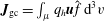$\boldsymbol{J}_{\text{gc}}=\int _{\unicode[STIX]{x1D707}}q_{h}\boldsymbol{u}\hat{f}\,\text{d}^{3}v$ , we have

(3.27) $$\begin{eqnarray}\displaystyle \frac{\unicode[STIX]{x1D6FF}l}{\unicode[STIX]{x1D6FF}\boldsymbol{A}}=\boldsymbol{J}_{\text{gc}}+\unicode[STIX]{x1D735}\times \boldsymbol{M}_{\text{gc}}-\unicode[STIX]{x1D707}_{0}^{-1}\unicode[STIX]{x1D735}\times \boldsymbol{B}, & & \displaystyle\end{eqnarray}$$

so that

(3.28) $$\begin{eqnarray}\displaystyle \boldsymbol{B}\times \frac{\unicode[STIX]{x1D6FF}l}{\unicode[STIX]{x1D6FF}\boldsymbol{A}}+\left(\unicode[STIX]{x1D735}\boldsymbol{\cdot }\frac{\unicode[STIX]{x1D6FF}l}{\unicode[STIX]{x1D6FF}\boldsymbol{A}}\right)\boldsymbol{A}=(\boldsymbol{J}-\boldsymbol{J}_{\text{gc}}-\unicode[STIX]{x1D735}\times \boldsymbol{M}_{\text{gc}})\times \boldsymbol{B}+(\unicode[STIX]{x1D735}\boldsymbol{\cdot }\boldsymbol{J}_{\text{gc}})\boldsymbol{A}. & & \displaystyle\end{eqnarray}$$

Then, upon adding the terms in (3.25) and (3.28), and by observing that

(3.29) $$\begin{eqnarray}\displaystyle \unicode[STIX]{x1D735}\boldsymbol{B}\boldsymbol{\cdot }\boldsymbol{M}_{\text{gc}}+\boldsymbol{B}\times \unicode[STIX]{x1D735}\times \boldsymbol{M}_{\text{gc}} & = & \displaystyle \unicode[STIX]{x1D735}\boldsymbol{\cdot }[(\boldsymbol{B}\boldsymbol{\cdot }\boldsymbol{M}_{\text{gc}})\mathbf{1}-\boldsymbol{B}\boldsymbol{M}_{\text{gc}}]\nonumber\\ \displaystyle & = & \displaystyle \unicode[STIX]{x1D735}\boldsymbol{\cdot }\int _{\unicode[STIX]{x1D707}}[\unicode[STIX]{x1D707}B(\mathbf{1}-\boldsymbol{b}\boldsymbol{b})-m_{h}(\boldsymbol{v}\boldsymbol{\cdot }\boldsymbol{b})\boldsymbol{b}\boldsymbol{w}_{\bot }]\hat{f}\,\text{d}^{3}v,\end{eqnarray}$$

equation (2.30) leads to

(3.30) $$\begin{eqnarray}\displaystyle \unicode[STIX]{x1D70C}\left(\frac{\unicode[STIX]{x2202}\boldsymbol{U}}{\unicode[STIX]{x2202}t}+\boldsymbol{U}\boldsymbol{\cdot }\unicode[STIX]{x1D735}\boldsymbol{U}\right)=-\unicode[STIX]{x1D735}\mathsf{p}-m_{h}\unicode[STIX]{x1D735}\boldsymbol{\cdot }\unicode[STIX]{x1D64B}_{\text{gc}}+\boldsymbol{J}\times \boldsymbol{B}. & & \displaystyle\end{eqnarray}$$

In the above, we have denoted

(3.31) $$\begin{eqnarray}\displaystyle \unicode[STIX]{x1D64B}_{\text{gc}}=\int _{\unicode[STIX]{x1D707}}[m_{h}(\boldsymbol{b}\boldsymbol{\cdot }\boldsymbol{v})^{2}\boldsymbol{b}\boldsymbol{b}+\unicode[STIX]{x1D707}B(\mathbf{1}-\boldsymbol{b}\boldsymbol{b})+m_{h}(\boldsymbol{b}\boldsymbol{\cdot }\boldsymbol{v})(\boldsymbol{w}_{\bot }\boldsymbol{b}+\boldsymbol{b}\boldsymbol{w}_{\bot })]\,\hat{f}\,\text{d}^{3}v, & & \displaystyle\end{eqnarray}$$

which reduces exactly to the expression (3.11), after integration over the perpendicular velocity coordinates $\boldsymbol{v}_{\bot }$ .

To summarize, we have obtained the following PCS equations for a hybrid kinetic-fluid model in the guiding center approximation

(3.32) $$\begin{eqnarray}\displaystyle \unicode[STIX]{x1D70C}\frac{\unicode[STIX]{x2202}\boldsymbol{U}}{\unicode[STIX]{x2202}t}+\unicode[STIX]{x1D70C}(\boldsymbol{U}\boldsymbol{\cdot }\unicode[STIX]{x1D735})\boldsymbol{U}=-\unicode[STIX]{x1D735}\mathsf{p}-\unicode[STIX]{x1D735}\boldsymbol{\cdot }\unicode[STIX]{x1D64B}_{\text{gc}}+\boldsymbol{J}\times \boldsymbol{B}, & & \displaystyle\end{eqnarray}$$

(3.33) $$\begin{eqnarray}\displaystyle \frac{\unicode[STIX]{x2202}\unicode[STIX]{x1D70C}}{\unicode[STIX]{x2202}t}+\unicode[STIX]{x1D735}\boldsymbol{\cdot }(\unicode[STIX]{x1D70C}\boldsymbol{U})=0,\quad \frac{\unicode[STIX]{x2202}\boldsymbol{B}}{\unicode[STIX]{x2202}t}=\unicode[STIX]{x1D735}\times (\boldsymbol{U}\times \boldsymbol{B}), & & \displaystyle\end{eqnarray}$$

(3.34) $$\begin{eqnarray}\displaystyle & & \displaystyle \frac{\unicode[STIX]{x2202}f}{\unicode[STIX]{x2202}t}+\unicode[STIX]{x1D735}\boldsymbol{\cdot }\left[\left((v_{\Vert }+U_{\Vert })\frac{\boldsymbol{B}^{\ast }}{B_{\Vert }^{\ast }}-\frac{\boldsymbol{b}}{B_{\Vert }^{\ast }}\times (\boldsymbol{E}^{\ast }-a_{h}^{-1}v_{\Vert }\unicode[STIX]{x1D735}U_{\Vert })\right)f\right]\nonumber\\ \displaystyle & & \displaystyle \quad +\,\unicode[STIX]{x2202}_{v_{\Vert }}\left[\frac{\boldsymbol{B}^{\ast }}{B_{\Vert }^{\ast }}\boldsymbol{\cdot }(a_{h}\boldsymbol{E}^{\ast }-v_{\Vert }\unicode[STIX]{x1D735}U_{\Vert })f\right]=0,\end{eqnarray}$$

with the definitions (3.5) and (3.11), and where $\boldsymbol{E}=-\boldsymbol{U}\times \boldsymbol{B}$ and $\boldsymbol{w}$ is given by (3.21). By construction, this system conserves energy and momentum. This system additionally allows for cross-helicity conservation, as proved in § 3.4.

We conclude by observing that the variational relation presented in § 2.4 between the CCS and the conservative PCS naturally extends to the case of guiding center motion by simply implementing the particle path decomposition (2.42). In the following section, we shall present one more variational approach connecting the two models.

3.3 An alternative variational approach

The original derivation of the conservative Vlasov PCS by Tronci (Reference Tronci2010) used an approach that is quite different from that employed in the previous section, which was modelled on the methods of Holm & Tronci (Reference Holm and Tronci2012). Starting from a Hamiltonian formulation of the conservative Vlasov CCS, Tronci (Reference Tronci2010) performed a change of dependent variables that exchanged the bulk fluid velocity with the total kinetic momentum density. Then the terms in the transformed Hamiltonian proportional to the momentum density carried by the kinetic population were dropped. This suggests that a similar approach might be available to derive the new PCS model in this article.

In this subsection we will demonstrate that our new PCS model may indeed be derived using an analogue of the approach used by Tronci (Reference Tronci2010). Moreover, in order to avoid working directly with field-theoretic Poisson brackets (which become quite cumbersome in this case), we will formulate our discussion in terms of phase space Lagrangians, which are known to provide a convenient bridge between the Hamiltonian and Lagrangian formalisms. The basic strategy will be as follows. First we will present the phase space Lagrangian underlying the (guiding center version of the) variational CCS presented by Burby & Tronci (Reference Burby and Tronci2017). Then we will perform a change of variables within the phase space Lagrangian from the bulk fluid velocity $\boldsymbol{u}$ to the total momentum variable $\boldsymbol{M}$ given in equation (3.8). Finally we will drop terms in the Hamiltonian part of the phase space Lagrangian that are proportional to the parallel momentum of the kinetic species. The resulting simplified transformed phase space Lagrangian will reproduce the conservative PCS given in equations (3.32)–(3.34). It is worth mentioning here that this alternative derivation avoids embedding the four-dimensional guiding center phase space into the six-dimensional Vlasov phase space; instead the four-dimensional guiding center phase space is employed directly throughout the discussion.

To begin, we restate the Euler–Poincaré formulation of the guiding center CCS given by Burby & Tronci (Reference Burby and Tronci2017) using a notation that is as consistent as possible with the notation used so far. The guiding center CCS Lagrangian is given by

(3.35) $$\begin{eqnarray}\displaystyle & & \displaystyle l_{\text{CCS}}(\boldsymbol{u},\unicode[STIX]{x1D70C},\boldsymbol{{\mathcal{X}}},f,\boldsymbol{A})=\frac{1}{2}\int \unicode[STIX]{x1D70C}|\boldsymbol{u}|^{2}\,\text{d}^{3}x-\int \unicode[STIX]{x1D70C}{\mathcal{U}}(\unicode[STIX]{x1D70C})\,\text{d}^{3}x-\frac{1}{2\unicode[STIX]{x1D707}_{0}}\int |\unicode[STIX]{x1D735}\times \boldsymbol{A}|^{2}\,\text{d}^{3}x\nonumber\\ \displaystyle & & \displaystyle \quad +\,\int _{\unicode[STIX]{x1D707}}f\left\{[m_{h}v_{\Vert }\boldsymbol{b}+q_{h}\boldsymbol{A}]\boldsymbol{\cdot }\boldsymbol{w}-\left[\frac{m_{h}}{2}v_{\Vert }^{2}+\unicode[STIX]{x1D707}B+q_{h}\boldsymbol{u}\boldsymbol{\cdot }\boldsymbol{A}\right]\right\}\,\text{d}^{4}z,\end{eqnarray}$$

where the symbols $(\boldsymbol{u},\unicode[STIX]{x1D70C},\boldsymbol{{\mathcal{X}}},f,\boldsymbol{A})$ now have slightly different meanings than in previous sections. The most critical difference is that the guiding center phase space consists of points $\boldsymbol{z}=(\boldsymbol{X},v_{\Vert })$ in a four-dimensional, rather than six-dimensional, space. The variable $\boldsymbol{u}$ is the velocity of the bulk fluid, which is expressed in terms of the bulk fluid configuration map $\boldsymbol{\unicode[STIX]{x1D702}}(\boldsymbol{x}_{0})$ according to $\dot{\boldsymbol{\unicode[STIX]{x1D702}}}(\boldsymbol{x}_{0})=\boldsymbol{u}(\boldsymbol{\unicode[STIX]{x1D702}}(\boldsymbol{x}_{0}))$ . The variable $\boldsymbol{{\mathcal{X}}}=(\boldsymbol{w},a_{\Vert })$ is the velocity of the kinetic species’ (four-dimensional) phase space fluid, which is similarly given in terms of the phase space fluid configuration map $\boldsymbol{z}(\boldsymbol{z}_{0})$ as $\dot{\boldsymbol{z}}(\boldsymbol{z}_{0})=\boldsymbol{{\mathcal{X}}}(\boldsymbol{z}(\boldsymbol{z}_{0}))$ . Finally, the variables $\unicode[STIX]{x1D70C}$ , $f$ and $\boldsymbol{A}$ are advected parameters given in terms of the fluid and phase space configuration maps, $\boldsymbol{\unicode[STIX]{x1D702}}$ and $\boldsymbol{z}$ , as in equation (2.23), but with $\boldsymbol{\unicode[STIX]{x1D702}}$ and $\boldsymbol{z}$ interpreted as just described, and $f$ is defined as in (3.3). Accordingly, the constrained variations associated with the advection relations (2.23) are modified according to

(3.36) $$\begin{eqnarray}\displaystyle \unicode[STIX]{x1D6FF}\unicode[STIX]{x1D70C}=-\unicode[STIX]{x1D735}\boldsymbol{\cdot }(\unicode[STIX]{x1D743}\unicode[STIX]{x1D70C}),\quad \unicode[STIX]{x1D6FF}f=-\unicode[STIX]{x1D735}_{\boldsymbol{z}}\boldsymbol{\cdot }(\unicode[STIX]{x1D729}f),\quad \unicode[STIX]{x1D6FF}\boldsymbol{A}=\unicode[STIX]{x1D743}\times \boldsymbol{B}-\unicode[STIX]{x1D735}(\unicode[STIX]{x1D743}\boldsymbol{\cdot }\boldsymbol{A}), & & \displaystyle\end{eqnarray}$$

and

(3.37) $$\begin{eqnarray}\displaystyle \unicode[STIX]{x1D6FF}\boldsymbol{u}=\unicode[STIX]{x2202}_{t}\unicode[STIX]{x1D743}+[\boldsymbol{u},\unicode[STIX]{x1D743}],\quad \unicode[STIX]{x1D6FF}\boldsymbol{{\mathcal{X}}}=\unicode[STIX]{x2202}_{t}\unicode[STIX]{x1D729}+[\boldsymbol{{\mathcal{X}}},\unicode[STIX]{x1D729}], & & \displaystyle\end{eqnarray}$$

where $\unicode[STIX]{x1D743}$ and $\unicode[STIX]{x1D729}$ are arbitrary vector fields on configuration space and four-dimensional phase space, respectively. The conservative guiding center CCS model then follows from the variational principle

(3.38) $$\begin{eqnarray}\displaystyle \unicode[STIX]{x1D6FF}\int _{t_{1}}^{t_{2}}l_{\text{CCS}}(\boldsymbol{u},\unicode[STIX]{x1D70C},\boldsymbol{{\mathcal{X}}},f,\boldsymbol{A})\,\text{d}t=0, & & \displaystyle\end{eqnarray}$$

which was shown by Burby & Tronci (Reference Burby and Tronci2017) to be equivalent to the system of equations (3.1)–(3.7).

Next we deduce the phase space Lagrangian for the guiding center CCS. More specifically, we would like to find a functional of the form

(3.39) $$\begin{eqnarray}\displaystyle L_{\text{CCS}}(\boldsymbol{\unicode[STIX]{x1D702}},\boldsymbol{u},\boldsymbol{z},\dot{\boldsymbol{\unicode[STIX]{x1D702}}},\dot{\boldsymbol{u}},\dot{\boldsymbol{z}};\unicode[STIX]{x1D70C}_{0},f_{0},\boldsymbol{A}_{0}), & & \displaystyle\end{eqnarray}$$

with an affine dependence on $\dot{\boldsymbol{\unicode[STIX]{x1D702}}},\dot{\boldsymbol{U}}$ and $\dot{\boldsymbol{z}}$ such that the following statement is true: the variational principle

(3.40) $$\begin{eqnarray}\displaystyle \unicode[STIX]{x1D6FF}\int _{t_{1}}^{t_{2}}L_{\text{CCS}}(\boldsymbol{\unicode[STIX]{x1D702}},\boldsymbol{u},\boldsymbol{z},\dot{\boldsymbol{\unicode[STIX]{x1D702}}},\dot{\boldsymbol{u}},\dot{\boldsymbol{z}};\unicode[STIX]{x1D70C}_{0},f_{0},\boldsymbol{A}_{0})\,\text{d}t=0, & & \displaystyle\end{eqnarray}$$

with $\boldsymbol{\unicode[STIX]{x1D702}},\boldsymbol{u}$ and $\boldsymbol{z}$ subjected to arbitrary variations with fixed endpoints, reproduces the guiding center CCS. The name ‘phase space Lagrangian’ is motivated by the fact that the guiding center CCS may be cast as a first-order ordinary differential equation (ODE) on the infinite-dimensional space consisting of tuples $(\boldsymbol{\unicode[STIX]{x1D702}},\boldsymbol{u},\boldsymbol{z})$ . It has been shown by Burby (Reference Burby2015) using a method inspired by Marsden, Patrick & Shkoller (Reference Marsden, Patrick and Shkoller1998) that there is a systematic procedure for deriving the phase space Lagrangian for any system with an Euler–Poincaré variational principle as soon as the structure of the initial value problem is understood. We refer to Burby (Reference Burby2015) for a detailed description of this procedure, which involves a careful study of the (temporal) boundary terms arising from the variational principle. When this procedure is applied to the guiding center CCS, we find that the appropriate phase space Lagrangian is given by

(3.41) $$\begin{eqnarray}\displaystyle L_{\text{CCS}} & = & \displaystyle \int \unicode[STIX]{x1D70C}\boldsymbol{u}\boldsymbol{\cdot }\boldsymbol{V}\text{d}^{3}x-\int q_{h}n_{h}\boldsymbol{A}\boldsymbol{\cdot }\boldsymbol{V}\,\text{d}^{3}x+\int _{\unicode[STIX]{x1D707}}f[q_{h}\boldsymbol{A}+m_{h}v_{\Vert }\boldsymbol{b}]\boldsymbol{\cdot }\boldsymbol{w}\,\text{d}^{4}z\nonumber\\ \displaystyle & & \displaystyle -\,{\mathcal{H}}_{\text{CCS}}(\boldsymbol{w},\unicode[STIX]{x1D70C},f,\boldsymbol{A}),\end{eqnarray}$$

where now $\boldsymbol{V}$ is given in terms of the bulk fluid configuration map as $\dot{\boldsymbol{\unicode[STIX]{x1D702}}}(\boldsymbol{x}_{0})=\boldsymbol{V}(\boldsymbol{\unicode[STIX]{x1D702}}(\boldsymbol{x}_{0}))$ , $\boldsymbol{{\mathcal{X}}}=(\boldsymbol{w},a_{\Vert })$ is defined as it was in equation (3.38) and the quantities $\unicode[STIX]{x1D70C},f$ and $\boldsymbol{A}$ are again given in terms of $\boldsymbol{\unicode[STIX]{x1D702}}$ and $\boldsymbol{z}$ according to equation (2.23). We stress that $\boldsymbol{u}$ plays the role of an independent generalized coordinate in $L_{\text{CCS}}$ ; we do not assume $\boldsymbol{u}=\boldsymbol{V}$ when defining $L_{\text{CCS}}$ . The CCS Hamiltonian is given by

(3.42) $$\begin{eqnarray}\displaystyle {\mathcal{H}}_{\text{CCS}} & = & \displaystyle \frac{1}{2}\int \unicode[STIX]{x1D70C}|\boldsymbol{u}|^{2}\,\text{d}^{3}x+\int \unicode[STIX]{x1D70C}{\mathcal{U}}(\unicode[STIX]{x1D70C})\,\text{d}^{3}x\nonumber\\ \displaystyle & & \displaystyle +\,\frac{1}{2\unicode[STIX]{x1D707}_{0}}\int |\boldsymbol{B}|^{2}\,\text{d}^{3}x+\int _{\unicode[STIX]{x1D707}}\left(\frac{m_{h}}{2}v_{\Vert }^{2}+\unicode[STIX]{x1D707}B\right)f\,\text{d}^{4}z.\end{eqnarray}$$

It is straightforward to show directly that the variational principle associated with $L_{\text{CCS}}$ reproduces the guiding center CCS.

The penultimate step in the derivation is to exploit the fact that, in the phase space variational principle (3.41), $\boldsymbol{u}$ plays the role of a generalized coordinate in the usual sense (Landau & Lifshitz Reference Landau and Lifshitz1976). We may therefore apply a point transformation to $\boldsymbol{u}$ without changing the form of the variational principle. In particular, if we pass into the new system of generalized coordinates defined by the transformation $(\boldsymbol{\unicode[STIX]{x1D702}},\boldsymbol{u},\boldsymbol{z})\mapsto (\boldsymbol{\unicode[STIX]{x1D702}},\boldsymbol{U},\boldsymbol{z})$ , where

(3.43) $$\begin{eqnarray}\displaystyle \boldsymbol{U}=\boldsymbol{u}+\unicode[STIX]{x1D70C}^{-1}\boldsymbol{b}\int _{\unicode[STIX]{x1D707}}m_{h}v_{\Vert }f\,\text{d}v_{\Vert } & & \displaystyle\end{eqnarray}$$

is the total kinetic momentum divided by the bulk mass density, i.e. $\boldsymbol{M}/\unicode[STIX]{x1D70C}$ , then

(3.44) $$\begin{eqnarray}\displaystyle \unicode[STIX]{x1D6FF}\int _{t_{1}}^{t_{2}}\bar{L}_{\text{CCS}}(\boldsymbol{\unicode[STIX]{x1D702}},\boldsymbol{U},\boldsymbol{z},\dot{\boldsymbol{\unicode[STIX]{x1D702}}},\dot{\boldsymbol{U}},\dot{\boldsymbol{z}};\unicode[STIX]{x1D70C}_{0},f_{0},\boldsymbol{A}_{0})\,\text{d}t=0, & & \displaystyle\end{eqnarray}$$

is a valid variational principle for the transformed guiding center CCS model, where $\bar{L}_{\text{CCS}}$ is the transformed CCS phase space Lagrangian and $\boldsymbol{U}$ is subjected to arbitrary variations. A trivial direct calculation shows that $\bar{L}_{\text{CCS}}$ is given by

(3.45) $$\begin{eqnarray}\displaystyle \bar{L}_{\text{CCS}} & = & \displaystyle \int \unicode[STIX]{x1D70C}\boldsymbol{U}\boldsymbol{\cdot }\boldsymbol{V}\,\text{d}^{3}x-\int _{\unicode[STIX]{x1D707}}fm_{h}v_{\Vert }\boldsymbol{b}\boldsymbol{\cdot }\boldsymbol{V}\,\text{d}^{4}z-\int q_{h}n_{h}\boldsymbol{A}\boldsymbol{\cdot }\boldsymbol{V}\,\text{d}^{3}x\nonumber\\ \displaystyle & & \displaystyle +\,\int _{\unicode[STIX]{x1D707}}f[q_{h}\boldsymbol{A}+m_{h}v_{\Vert }\boldsymbol{b}]\boldsymbol{\cdot }\boldsymbol{w}\,\text{d}^{4}z-\overline{{\mathcal{H}}}_{\text{CCS}}(\boldsymbol{U},\unicode[STIX]{x1D70C},f,\boldsymbol{A}),\end{eqnarray}$$

where the transformed Hamiltonian is given by

(3.46) $$\begin{eqnarray}\displaystyle \overline{{\mathcal{H}}}_{\text{CCS}}(\boldsymbol{U},\unicode[STIX]{x1D70C},f,\boldsymbol{A})={\mathcal{H}}_{\text{CCS}}\left(\boldsymbol{U}-\unicode[STIX]{x1D70C}^{-1}\boldsymbol{b}\int _{\unicode[STIX]{x1D707}}m_{h}v_{\Vert }f\,\text{d}v_{\Vert },\unicode[STIX]{x1D70C},f,\boldsymbol{A}\right). & & \displaystyle\end{eqnarray}$$

We conclude the derivation as follows. Because we assume that the kinetic population is rarefied, we have

(3.47) $$\begin{eqnarray}\displaystyle {\mathcal{H}}_{\text{CCS}}\left(\boldsymbol{U}-\unicode[STIX]{x1D70C}^{-1}\boldsymbol{b}\int _{\unicode[STIX]{x1D707}}m_{h}v_{\Vert }f\,\text{d}v_{\Vert },\unicode[STIX]{x1D70C},f,\boldsymbol{A}\right)\approx {\mathcal{H}}_{\text{CCS}}(\boldsymbol{U},\unicode[STIX]{x1D70C},f,\boldsymbol{A}). & & \displaystyle\end{eqnarray}$$

This motivates us to mimic the key step in the Hamiltonian derivation of the Vlasov PCS of Tronci (Reference Tronci2010) by defining

(3.48) $$\begin{eqnarray}\displaystyle {\mathcal{H}}_{\text{PCS}}(\boldsymbol{U},\unicode[STIX]{x1D70C},f,\boldsymbol{A})\equiv {\mathcal{H}}_{\text{CCS}}(\boldsymbol{U},\unicode[STIX]{x1D70C},f,\boldsymbol{A}), & & \displaystyle\end{eqnarray}$$

to be the PCS Hamiltonian, and

(3.49) $$\begin{eqnarray}\displaystyle L_{\text{PCS}} & = & \displaystyle \int \unicode[STIX]{x1D70C}\boldsymbol{U}\boldsymbol{\cdot }\boldsymbol{V}\,\text{d}^{3}x-\int _{\unicode[STIX]{x1D707}}fm_{h}v_{\Vert }\boldsymbol{b}\boldsymbol{\cdot }\boldsymbol{V}\,\text{d}^{4}z-\int q_{h}n_{h}\boldsymbol{A}\boldsymbol{\cdot }\boldsymbol{V}\,\text{d}^{3}x\nonumber\\ \displaystyle & & \displaystyle +\,\int _{\unicode[STIX]{x1D707}}f[q_{h}\boldsymbol{A}+m_{h}v_{\Vert }\boldsymbol{b}]\boldsymbol{\cdot }\boldsymbol{w}\,\text{d}^{4}z-{\mathcal{H}}_{\text{PCS}}(\boldsymbol{U},\unicode[STIX]{x1D70C},f,\boldsymbol{A}),\end{eqnarray}$$

to be the PCS phase space Lagrangian. Our putative guiding center PCS model is then defined by the variational principle

(3.50) $$\begin{eqnarray}\displaystyle \unicode[STIX]{x1D6FF}\int _{t_{1}}^{t_{2}}L_{\text{PCS}}(\boldsymbol{\unicode[STIX]{x1D702}},\boldsymbol{U},\boldsymbol{z},\dot{\boldsymbol{\unicode[STIX]{x1D702}}},\dot{\boldsymbol{U}},\dot{\boldsymbol{z}};\unicode[STIX]{x1D70C}_{0},f_{0},\boldsymbol{A}_{0})\,\text{d}t=0, & & \displaystyle\end{eqnarray}$$

where $\boldsymbol{\unicode[STIX]{x1D702}},\boldsymbol{U}$ and $\boldsymbol{z}$ are subjected to arbitrary variations with fixed endpoints. If the Euler–Lagrange equations associated with this variational principle reproduce the conservative guiding center PCS model presented in § 3.2, we will have succeeded in proving the validity of this alternative derivation.

We can see that the variational principle (3.50) does indeed reproduce the conservative guiding center PCS model (3.32)–(3.34) as follows. In the action principle (3.50), variations of $\boldsymbol{z}$ , $\boldsymbol{U}$ and $\boldsymbol{\unicode[STIX]{x1D702}}$ lead to the conditions

(3.51) $$\begin{eqnarray}\displaystyle & \displaystyle q_{h}\boldsymbol{E}_{\text{PCS}}^{\ast }+q_{h}\boldsymbol{w}\times \boldsymbol{B}^{\ast }-m_{h}a_{\Vert }\boldsymbol{b}=0, & \displaystyle\end{eqnarray}$$

(3.52) $$\begin{eqnarray}\displaystyle & \displaystyle m_{h}\boldsymbol{b}\boldsymbol{\cdot }\boldsymbol{w}-m_{h}\boldsymbol{b}\boldsymbol{\cdot }\boldsymbol{V}-\unicode[STIX]{x2202}_{v_{\Vert }}\frac{\unicode[STIX]{x1D6FF}{\mathcal{H}}_{\text{PCS}}}{\unicode[STIX]{x1D6FF}f}=0, & \displaystyle\end{eqnarray}$$

(3.53) $$\begin{eqnarray}\displaystyle & \displaystyle \unicode[STIX]{x1D70C}\boldsymbol{V}-\frac{\unicode[STIX]{x1D6FF}{\mathcal{H}}_{\text{PCS}}}{\unicode[STIX]{x1D6FF}\boldsymbol{U}}=0, & \displaystyle\end{eqnarray}$$

(3.54) $$\begin{eqnarray}\displaystyle & & \displaystyle \unicode[STIX]{x1D70C}(\unicode[STIX]{x2202}_{t}\boldsymbol{u}_{\text{PCS}}+(\unicode[STIX]{x1D735}\times \boldsymbol{u}_{\text{PCS}})\times \boldsymbol{V}+\unicode[STIX]{x1D735}(\boldsymbol{u}_{\text{PCS}}\boldsymbol{\cdot }\boldsymbol{V}))+\unicode[STIX]{x1D70C}\unicode[STIX]{x1D735}\left(\frac{\unicode[STIX]{x1D6FF}{\mathcal{H}}_{\text{PCS}}}{\unicode[STIX]{x1D6FF}\unicode[STIX]{x1D70C}}-\boldsymbol{U}\boldsymbol{\cdot }\boldsymbol{V}\right)\nonumber\\ \displaystyle & & \displaystyle \quad =\boldsymbol{J}_{\text{PCS}}\times \boldsymbol{B}-\boldsymbol{A}\unicode[STIX]{x1D735}\boldsymbol{\cdot }\frac{\unicode[STIX]{x1D6FF}{\mathcal{H}}_{\text{PCS}}}{\unicode[STIX]{x1D6FF}\boldsymbol{A}},\end{eqnarray}$$

respectively, where $\boldsymbol{B}^{\ast }$ is given in equation (3.5), and

(3.55) $$\begin{eqnarray}\displaystyle & \displaystyle \boldsymbol{J}_{\text{PCS}}=\frac{\unicode[STIX]{x1D6FF}{\mathcal{H}}_{\text{PCS}}}{\unicode[STIX]{x1D6FF}\boldsymbol{A}}-q_{h}\int _{\unicode[STIX]{x1D707}}(\boldsymbol{w}-\boldsymbol{V})f\,\text{d}v_{\Vert }-\unicode[STIX]{x1D735}\times \int _{\unicode[STIX]{x1D707}}\frac{m_{h}v_{\Vert }}{B}(\boldsymbol{w}-\boldsymbol{V})_{\bot }f\,\text{d}v_{\Vert }, & \displaystyle\end{eqnarray}$$

(3.56) $$\begin{eqnarray}\displaystyle & \displaystyle \boldsymbol{u}_{\text{PCS}}=\boldsymbol{U}-\unicode[STIX]{x1D70C}^{-1}\boldsymbol{b}\int _{\unicode[STIX]{x1D707}}m_{h}v_{\Vert }f\,\text{d}v_{\Vert }, & \displaystyle\end{eqnarray}$$

(3.57) $$\begin{eqnarray}\displaystyle & \displaystyle \boldsymbol{E}_{\text{PCS}}^{\ast }=-\boldsymbol{V}\times \boldsymbol{B}-\frac{m_{h}}{q_{h}}\frac{v_{\Vert }}{B}\unicode[STIX]{x1D735}\times (\boldsymbol{V}\times \boldsymbol{B})_{\bot }-\frac{1}{q_{h}}\unicode[STIX]{x1D735}\left(\frac{\unicode[STIX]{x1D6FF}{\mathcal{H}}_{\text{PCS}}}{\unicode[STIX]{x1D6FF}f}+m_{h}v_{\Vert }\boldsymbol{b}\boldsymbol{\cdot }\boldsymbol{V}\right), & \displaystyle\end{eqnarray}$$

is convenient shorthand notation. By making use of the functional derivative relations

(3.58) $$\begin{eqnarray}\displaystyle \frac{\unicode[STIX]{x1D6FF}{\mathcal{H}}_{\text{PCS}}}{\unicode[STIX]{x1D6FF}f}=\unicode[STIX]{x1D707}B+\frac{m_{h}}{2}v_{\Vert }^{2},\quad \frac{\unicode[STIX]{x1D6FF}{\mathcal{H}}_{\text{PCS}}}{\unicode[STIX]{x1D6FF}\boldsymbol{ U}}=\unicode[STIX]{x1D70C}\boldsymbol{U},\quad \frac{\unicode[STIX]{x1D6FF}{\mathcal{H}}_{\text{PCS}}}{\unicode[STIX]{x1D6FF}\unicode[STIX]{x1D70C}}=\frac{1}{2}|\boldsymbol{U}|^{2}+{\mathcal{U}}+\unicode[STIX]{x1D70C}{\mathcal{U}}^{\prime },\qquad & & \displaystyle\end{eqnarray}$$

(3.59) $$\begin{eqnarray}\displaystyle \frac{\unicode[STIX]{x1D6FF}{\mathcal{H}}_{\text{PCS}}}{\unicode[STIX]{x1D6FF}\boldsymbol{ A}}=\unicode[STIX]{x1D735}\times \left(\unicode[STIX]{x1D707}_{0}^{-1}\boldsymbol{B}+\boldsymbol{b}\int _{\unicode[STIX]{x1D707}}\unicode[STIX]{x1D707}f\,\text{d}v_{\Vert }\right), & & \displaystyle\end{eqnarray}$$

and applying the following non-trivial intermediate consequence of the Euler–Lagrange equations:

(3.60) $$\begin{eqnarray}\displaystyle \unicode[STIX]{x2202}_{t}\left(\boldsymbol{b}\int _{\unicode[STIX]{x1D707}}m_{h}v_{\Vert }f\,\text{d}v_{\Vert }\right) & = & \displaystyle q_{h}\left(\int _{\unicode[STIX]{x1D707}}(\boldsymbol{w}-\boldsymbol{V})f\,\text{d}v_{\Vert }\right)\times \boldsymbol{B}+\unicode[STIX]{x1D735}\boldsymbol{b}\boldsymbol{\cdot }m_{h}\int _{\unicode[STIX]{x1D707}}v_{\Vert }\boldsymbol{w}_{\bot }f\,\text{d}v_{\Vert }\nonumber\\ \displaystyle & & \displaystyle -\,\frac{\unicode[STIX]{x1D735}B}{B}\int _{\unicode[STIX]{x1D707}}\unicode[STIX]{x1D707}Bf\,\text{d}v_{\Vert }-\unicode[STIX]{x1D735}\boldsymbol{\cdot }\left(m_{h}\int _{\unicode[STIX]{x1D707}}v_{\Vert }\boldsymbol{w}\boldsymbol{b}f\,\text{d}v_{\Vert }\right),\end{eqnarray}$$

it is straightforward to show that equations (3.51)–(3.54) recover (3.32)–(3.34).

3.4 Discussion and conservation laws

The conservative PCS scheme (3.32)–(3.34) differs from other PCS schemes appearing in the literature in many ways. Probably, the most direct comparison is with the analogue scheme proposed by Park et al. (Reference Park, Belova, Fu, Tang, Strauss and Sugiyama1999, see § III.C). Although the exact expression of the pressure tensor is not specified in that work, the corresponding guiding center trajectories can be immediately compared to our kinetic equation (3.34). We can report two main differences: the first is that Park et al. (Reference Park, Belova, Fu, Tang, Strauss and Sugiyama1999) used the approximation $B_{\Vert }^{\ast }\simeq B$ , while the second more important difference is that the inertial force terms involving the bulk fluid velocity in (3.34) are totally absent. This is the conventional approach used in the literature to produce PCS models, which destroys the correct energy balance, as we discussed earlier on.

It would also be tempting to compare the PCS system (3.32)–(3.34) with other work on the same topic. However, many variants have been proposed and a direct comparison is not always clear. For example, Kim et al. (Reference Kim, Sovinec and Parker2004), Kim & the NIMROD team (Reference Kim2008) and Takahashi et al. (Reference Takahashi, Brennan and Kim2009a ) use the definition of pressure involving the relative velocity, that is $\widetilde{\unicode[STIX]{x1D64B}}_{h}=m_{h}\int (\boldsymbol{v}-\boldsymbol{V})(\boldsymbol{v}-\boldsymbol{V})f\,\text{d}^{3}v$ . As Tronci (Reference Tronci2010) and Holm & Tronci (Reference Holm and Tronci2012) showed by using full Vlasov kinetics, this form of the pressure tensor can be obtained in an energy-conserving model by decomposing the total energy of the energetic particle and then discarding the mean flow terms while retaining temperature terms. While this approximation is physically very appealing, the resulting energy-conserving equations are much more complicated, which is why we decided to retain the full stress tensor $\unicode[STIX]{x1D64B}_{h}=m_{h}\int \boldsymbol{v}\boldsymbol{v}f\,\text{d}^{3}v$ in the equations of motion. However, inertial force terms still appear in the energetic particle motion (Tronci Reference Tronci2010; Holm & Tronci Reference Holm and Tronci2012), and these forces are completely absent in the literature.

Elsewhere (Cheng Reference Cheng1991; Briguglio et al. Reference Briguglio, Vlad, Zonca and Kar1995; Fu & Park Reference Fu and Park1995; Briguglio, Vlad & Zonca Reference Briguglio, Vlad and Zonca1998; Fu et al. Reference Fu, Park, Strauss, Breslau, Chen, Jardin and Sugiyama2006), variants of the CGL stress tensor $\unicode[STIX]{x1D64B}_{\text{CGL}}=m_{h}\int _{\unicode[STIX]{x1D707}}[v_{\Vert }^{2}\boldsymbol{b}\boldsymbol{b}+\unicode[STIX]{x1D707}B(\mathbf{1}-\boldsymbol{b}\boldsymbol{b})]f\,\text{d}v_{\Vert }$ are retained in the fluid momentum equation and the energetic particles are described by gyrokinetics. While this case is not treated in this paper (see Burby & Tronci Reference Burby and Tronci2017, for conservative CCS models using gyrokinetics) we may still comment that inertial forces would still be expected to emerge in the gyrokinetic formalism for fully nonlinear conservative PCS models.

The system (3.32)–(3.34) has been constructed within the Euler–Poincaré variational framework by exploiting the coupling between fluid and phase space paths and their Eulerian variable counterparts. As we anticipated, energy conservation follows by construction for the following energy functional (Hamiltonian):

(3.61) $$\begin{eqnarray}\displaystyle E=\frac{1}{2}\int \unicode[STIX]{x1D70C}|\boldsymbol{U}|^{2}\,\text{d}^{3}x+\int _{\unicode[STIX]{x1D707}}\left(\frac{m_{h}}{2}v_{\Vert }^{2}+\unicode[STIX]{x1D707}B\right)f\,\text{d}v_{\Vert }\,\text{d}^{3}x+\int \unicode[STIX]{x1D70C}{\mathcal{U}}(\unicode[STIX]{x1D70C})\,\text{d}^{3}x+\frac{1}{2\unicode[STIX]{x1D707}_{0}}\int |\boldsymbol{B}|^{2}\,\text{d}^{3}x. & & \displaystyle \nonumber\\ \displaystyle & & \displaystyle\end{eqnarray}$$

This is the sum of the bulk MHD total energy and the energy of the guiding center ensemble for the energetic particles. Notice that this coincides with the same energy functional that is conserved by the CCS system (3.1)–(3.4).

Other than energy conservation, the PCS model (3.32)–(3.34) also enjoys cross-helicity conservation, as it emerges from direct application of equation (2.36). To see this, we recall the definition $\boldsymbol{K}_{\text{gc}}=m_{h}\int _{\unicode[STIX]{x1D707}}(\boldsymbol{b}\boldsymbol{\cdot }\boldsymbol{v})\hat{f}\,\text{d}^{3}v$ and write (2.36) more explicitly as

(3.62) $$\begin{eqnarray}\displaystyle \left(\frac{\unicode[STIX]{x2202}}{\unicode[STIX]{x2202}t}+\unicode[STIX]{x00A3}_{\boldsymbol{U}}\right)(\unicode[STIX]{x1D70C}\boldsymbol{U}-\boldsymbol{K}_{\text{gc}}-q_{h}n_{h}\boldsymbol{A}) & = & \displaystyle \unicode[STIX]{x1D70C}\unicode[STIX]{x1D735}\left[\frac{U^{2}}{2}-{\mathcal{U}}-\unicode[STIX]{x1D70C}{\mathcal{U}}^{\prime }\right]\nonumber\\ \displaystyle & & \displaystyle +\,(\boldsymbol{J}-\boldsymbol{J}_{\text{gc}}-\unicode[STIX]{x1D735}\times \boldsymbol{M}_{\text{gc}})\times \boldsymbol{B}+(\unicode[STIX]{x1D735}\boldsymbol{\cdot }\boldsymbol{J}_{\text{gc}})\boldsymbol{A},\qquad\end{eqnarray}$$

that is, using (2.31) and $q_{h}\unicode[STIX]{x2202}_{t}n_{h}+\unicode[STIX]{x1D735}\boldsymbol{\cdot }(q_{h}n_{h}\boldsymbol{U}+\boldsymbol{J}_{\text{gc}})=0$ ,

(3.63) $$\begin{eqnarray}\displaystyle \left(\frac{\unicode[STIX]{x2202}}{\unicode[STIX]{x2202}t}+\boldsymbol{U}\boldsymbol{\cdot }\unicode[STIX]{x1D735}+\unicode[STIX]{x1D735}\boldsymbol{U}\boldsymbol{\cdot }\right)(\boldsymbol{U}-\unicode[STIX]{x1D70C}^{-1}\boldsymbol{K}_{\text{gc}}) & = & \displaystyle \,\unicode[STIX]{x1D735}\left[\frac{U^{2}}{2}-{\mathcal{U}}-\unicode[STIX]{x1D70C}{\mathcal{U}}^{\prime }\right]\nonumber\\ \displaystyle & & \displaystyle +\,\unicode[STIX]{x1D70C}^{-1}(\boldsymbol{J}-\boldsymbol{J}_{\text{gc}}-\unicode[STIX]{x1D735}\times \boldsymbol{M}_{\text{gc}})\times \boldsymbol{B}.\qquad\end{eqnarray}$$

Then, by dotting equation (3.63) with $\boldsymbol{B}$ and integrating, we obtain conservation of the following cross-helicity

(3.64) $$\begin{eqnarray}\displaystyle \frac{\text{d}}{\text{d}t}\int \boldsymbol{B}\boldsymbol{\cdot }(\boldsymbol{U}-\unicode[STIX]{x1D70C}^{-1}\boldsymbol{K}_{\text{gc}})\,\text{d}^{3}x=0, & & \displaystyle\end{eqnarray}$$

which is the guiding center analogue of the full-orbit Vlasov correspondent (2.28). In addition, the standard frozen-in condition also ensures conservation of magnetic helicity. We remark that, while the latter is also preserved by the non-conservative models appearing in the literature, cross-helicity conservation is a specific feature of the new PCS model (3.32)–(3.34) and it is lost in other models. As a final remark, we notice that cross-helicity can be exploited to perform Lyapunov stability studies (Holm et al. Reference Holm, Marsden, Ratiu and Weinstein1985) along the lines of those already carried out for the case of the Vlasov PCS model (2.14)–(2.16) (Morrison et al. Reference Morrison, Tassi, Tronci, Kirillov and Pelinovsky2014; Tronci et al. Reference Tronci, Tassi and Morrison2015).