1 Introduction
Supercritical free-surface flows can experience a sudden change in flow conditions caused, for instance, by the presence of an obstruction, which produces a thicker and much slower flow, subcritical and able to propagate in the direction opposite to the incoming stream. The discontinuity in height and velocity, namely the normal jump, demarcates the transition between the incoming supercritical flow and the outgoing subcritical flow. Under certain conditions, an equilibrium is met and standing jumps can be produced. Standing jumps have been observed in various experiments for a wide range of free-surface flows involving different fluids. There exist a great number of experiments on water flows in air, as reviewed by Chanson (Reference Chanson2009a ). Standing jumps have also been observed in other fluids, such as flows of oil – or oil mixture – in water (Yih & Guha Reference Yih and Guha1955), and flows of granular materials in air, as reported in the recent experimental study by Faug et al. (Reference Faug, Childs, Wyburn and Einav2015) and a number of valuable references therein.
Standing jumps in free-surface flows are ubiquitous in many real-world engineering applications. For instance, the design of dissipative structures in interaction with large-scale flows, such as energy dissipators used in hydraulics (Hager Reference Hager1992) or protection dams against avalanches (Barbolini et al. Reference Barbolini, Domaas, Faug, Gauer, Hakonardottir, Harbitz, Issler, Johannesson, Lied and Naaïm2009), needs a robust prediction of the jump heights in a broad range of flow conditions. These practical applications have motivated several theoretical, experimental and numerical studies. However, prediction of the heights of normal standing jumps for any kind of fluid, including water, and under different flow boundary conditions, is still a challenging question in fluid mechanics.
The following equation, known as the Bélanger equation (see Chanson (Reference Chanson2009b )), and derived from mass and momentum balances across the jump discontinuity,
 $$\begin{eqnarray}\frac{h_{\ast }}{h}=\frac{1}{2}\left(\sqrt{1+8Fr_{0}^{2}}-1\right),\end{eqnarray}$$
was initially developed for horizontal water flows to predict the height
 $h_{\ast }$
of the standing jump relative to the height
 $h$
of the supercritical incoming flow. It predicts a one-to-one relation between the sequent depth ratio
 $h_{\ast }/h$
and the Froude number defined by
 $Fr_{0}=\bar{u}/\sqrt{gh}$
(equation (1.1) is only valid for supercritical incoming flows, meaning that
 $Fr_{0}>1$
). The Froude number is the ratio of the depth-averaged velocity
 $\bar{u}$
to the speed of gravity waves
 $\sqrt{gh}$
. The Bélanger equation is a Rankine–Hugoniot relation in the sense that it considers the jump as a mathematical discontinuity, thus ignoring – or neglecting – the finite length of the jump itself. In other words, the Bélanger equation states that the jump height would only depend on the velocity and the height of the incoming flow. However, it is most likely that under certain conditions volume forces, namely the component of the jump weight along the slope (for flows down an incline) and/or the resistive friction force, can come into play. Furthermore, the Bélanger equation does not consider any change in density across the jump which may occur when the incoming flow is compressible. The traditional Bélanger equation is therefore valid for jumps formed in incompressible and frictionless fluids on a horizontal and smooth bottom.
The present paper revisits a number of experimental data sets, showing that the Bélanger equation fails in predicting the jump height because at least one assumption made to establish the Bélanger equation is violated by the experimental conditions and/or the fluid rheology at stake. The overarching aim of the paper is to overcome the gap between the prediction from the Bélanger equation and existing experiments, using a universal relation for the height of standing jumps. A general solution, which takes into account the forces acting over the finite length of the jump, as well as the density change across the jump, is derived. It is then validated on a number of laboratory data sets available in the literature, provided that minimal assumptions are made for the closure relations associated with the resistive friction force within the jump volume.
We apply mass and momentum conservation equations over the finite length of the jump. This allows us to establish a cubic equation that can be solved by Cardano’s method (Cardano & Spon Reference Cardano and Spon1968). We revisit and cross-compare relevant experimental data on jumps involving water flows on horizontal and inclined planes, over smooth or rough beds, as well as dense and dilute flows of granular materials down inclined planes (§ 3). Each term contributing to the general relation can be analysed and carefully checked against the various existing experiments, which allows us to highlight the robustness of this general relation in all situations. The relation is used to calibrate relevant friction closure laws for both water and granular jumps (§ 4). However, the general relation can predict the height of the jump only if another length scale, namely the length of the jump, is known. As this crucial question is not yet resolved, we end § 4 by proposing empirical but simple closure relations for the jump length. Section 5 summarizes the main outcomes of our study and concludes on the need for new developments regarding the length of standing normal jumps.
2 General relation for standing jumps
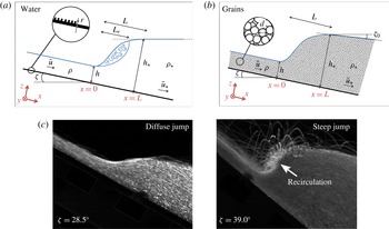
We consider a free-surface flow – of either water or dry grains – down an incline, as shown in figure 1. Figure 1(c) displays two pictures of granular jumps observed in laboratory tests by Faug et al. (Reference Faug, Childs, Wyburn and Einav2015): a diffuse jump at low slope angle and a steep jump, with the presence of recirculation, at high slope angle. The slope of the incline is called
 $\unicode[STIX]{x1D701}$
. The depth-averaged velocity, the density and the height (perpendicular to the bottom) of the flow are respectively
 $\bar{u}$
,
 $\unicode[STIX]{x1D70C}$
and
 $h$
before the jump, and
 $\bar{u}_{\ast }$
,
 $\unicode[STIX]{x1D70C}_{\ast }$
and
 $h_{\ast }$
after the jump. The jump length
 $L$
is taken parallel to the bottom (see its exact definition in § 3.1). When the bottom is rough, we introduce the parameter
 $r$
, which is the mean height of the roughness (see figure 1
a).
Sketches of stationary jumps made of water (a) and dry grains (b), with
 $\bar{u}$
,
 $\unicode[STIX]{x1D70C}$
and
 $h$
the incoming depth-averaged velocity, density and height. The subscript star
 $\ast$
refers to the values of velocity, density and height after the jump. Here,
 $\unicode[STIX]{x1D701}$
is the slope of the channel,
 $L$
is the length of the jump and
 $r$
represents the mean size of the roughness. In the case of water, some authors (see Carollo, Ferro & Pampalone (Reference Carollo, Ferro and Pampalone2007) for instance) did not measure the jump length but the length of the roller,
 $L_{r}$
, which is a little smaller than the jump length, as shown in (a). In the case of a granular flow, the outgoing flow is not horizontal but inclined at a constant angle with the horizontal, which corresponds to the limit angle below which no jump can form (see more details in Faug et al. (Reference Faug, Childs, Wyburn and Einav2015)). The images in (c) show two granular jumps observed by Faug et al. (Reference Faug, Childs, Wyburn and Einav2015), a diffuse jump for a low slope angle and a low Froude number, and a steep jump with recirculation for a large slope angle and a large Froude number.

The jump is defined as the part of the flow between the upstream supercritical flow and the downstream subcritical flow, both at equilibrium. In this definition, the jump cannot be considered as a shock, as done, for instance, in Hákonardóttir & Hogg (Reference Hákonardóttir and Hogg2005), Gray & Cui (Reference Gray and Cui2007) and Vreman et al. (Reference Vreman, Al-Tarazi, Kuipers, van Sint Annaland and Bokhove2007). In contrast to a shock, the jump has a finite length
 $L$
and then a volume on which forces come into play. We apply mass and momentum conservation equations in their depth-averaged forms under steady-state conditions to this jump volume, in a similar fashion to that initially proposed by Savage (Reference Savage1979) for granular flows, and earlier by Chow (Reference Chow1959) for water flows. In addition, we take into account the density change across the jump, as recently considered by Faug et al. (Reference Faug, Childs, Wyburn and Einav2015). The forces that apply on the jump volume are the weight of the jump
 $w$
(see its expression in § 2.1), the effective frictional force acting over the jump length
 $\unicode[STIX]{x1D70F}_{b}$
(see its expressions in §§ 2.1 and 2.2 for dry grains and water respectively) and the pressure forces acting on each side of the jump, which are assumed to be hydrostatic. The depth-averaged equations of mass and momentum conservation projected on the
 $x$
axis (along the slope of the incline) read as follows:
 $$\begin{eqnarray}\displaystyle & \displaystyle \unicode[STIX]{x1D70C}\bar{u}h=\unicode[STIX]{x1D70C}_{\ast }\bar{u}_{\ast }h_{\ast }, & \displaystyle\end{eqnarray}$$
 $$\begin{eqnarray}\displaystyle & \displaystyle \unicode[STIX]{x1D6FD}_{\ast }\unicode[STIX]{x1D70C}_{\ast }{\bar{u}_{\ast }}^{2}h_{\ast }-\unicode[STIX]{x1D6FD}\unicode[STIX]{x1D70C}\bar{u}^{2}h={\textstyle \frac{1}{2}}k\unicode[STIX]{x1D70C}gh^{2}\cos \unicode[STIX]{x1D701}-{\textstyle \frac{1}{2}}k_{\ast }\unicode[STIX]{x1D70C}g{h_{\ast }}^{2}\cos \unicode[STIX]{x1D701}+w\sin \unicode[STIX]{x1D701}-\unicode[STIX]{x1D70F}_{b}L, & \displaystyle\end{eqnarray}$$
where
 $k$
(respectively
 $k_{\ast }$
) and
 $\unicode[STIX]{x1D6FD}$
(respectively
 $\unicode[STIX]{x1D6FD}_{\ast }$
) hold for the earth pressure and Boussinesq momentum coefficients before (respectively after) the jump, as will be discussed in more detail in § 3.6.
2.1 Standing granular jumps
For a flow of dry granular material down an incline, the effective frictional stress acting over the jump length can be expressed as a Coulomb-like stress:
 $$\begin{eqnarray}\unicode[STIX]{x1D70F}_{b}=\unicode[STIX]{x1D707}_{e}\frac{w}{L}\cos \unicode[STIX]{x1D701},\end{eqnarray}$$
where
 $\unicode[STIX]{x1D707}_{e}$
holds for the effective coefficient of friction, which includes all of the sources of friction over the jump length. A depth-averaged friction law for
 $\unicode[STIX]{x1D707}_{e}$
estimated over the entire length of the jump will be proposed in § 3.5.2. Combination of (2.3) with the continuity equations (2.1) and (2.2) yields the following relation for a granular fluid down an incline:
 $$\begin{eqnarray}Fr^{2}\left(\unicode[STIX]{x1D6FD}-\frac{\unicode[STIX]{x1D6FD}_{\ast }}{\displaystyle \frac{\unicode[STIX]{x1D70C}_{\ast }}{\unicode[STIX]{x1D70C}}\frac{h_{\ast }}{h}}\right)=\frac{1}{2}\left[k_{\ast }\frac{\unicode[STIX]{x1D70C}_{\ast }}{\unicode[STIX]{x1D70C}}\left(\frac{h_{\ast }}{h}\right)^{2}-k-K_{0}\frac{L}{h}\left(1+\frac{\unicode[STIX]{x1D70C}_{\ast }}{\unicode[STIX]{x1D70C}}\frac{h_{\ast }}{h}\right)(\tan \unicode[STIX]{x1D701}-\unicode[STIX]{x1D707}_{e})\right].\end{eqnarray}$$
The Froude number
 $Fr$
takes into account the slope,
 $Fr=\bar{u}/\sqrt{gh\cos \unicode[STIX]{x1D701}}$
. We define the shape factor
 $K_{0}$
so that the weight per unit width of the jump can be written as
 $w=K_{0}gL(\unicode[STIX]{x1D70C}h+\unicode[STIX]{x1D70C}_{\ast }h_{\ast })/2$
, as initially introduced by Savage (Reference Savage1979). In other words, we have
 $$\begin{eqnarray}K_{0}=\frac{2\displaystyle \int _{0}^{L}\unicode[STIX]{x1D70C}(x){\mathcal{Z}}(x)\,\text{d}x}{L(\unicode[STIX]{x1D70C}h+\unicode[STIX]{x1D70C}_{\ast }h_{\ast })},\end{eqnarray}$$
where
 $\unicode[STIX]{x1D70C}(x)$
and
 ${\mathcal{Z}}(x)$
are the density and the height of the flow inside the jump.
Equation (2.4) can be rearranged in the form of a cubic equation:
 $$\begin{eqnarray}\left(\frac{h_{\ast }}{h}\right)^{3}+A_{g}\left(\frac{h_{\ast }}{h}\right)^{2}+B_{g}\frac{h_{\ast }}{h}+C_{g}=0,\end{eqnarray}$$
where
 $A_{g}$
,
 $B_{g}$
and
 $C_{g}$
are defined by
 $$\begin{eqnarray}\displaystyle & \displaystyle A_{g}=-\frac{L}{h}\frac{K_{0}}{k_{\ast }}(\tan \unicode[STIX]{x1D701}-\unicode[STIX]{x1D707}_{e}), & \displaystyle\end{eqnarray}$$
 $$\begin{eqnarray}\displaystyle & \displaystyle B_{g}=-\frac{2\unicode[STIX]{x1D6FD}Fr^{2}+k+K_{0}\displaystyle \frac{L}{h}(\tan \unicode[STIX]{x1D701}-\unicode[STIX]{x1D707}_{e})}{k_{\ast }\displaystyle \frac{\unicode[STIX]{x1D70C}_{\ast }}{\unicode[STIX]{x1D70C}}}, & \displaystyle\end{eqnarray}$$
 $$\begin{eqnarray}\displaystyle & \displaystyle C_{g}=\frac{2\unicode[STIX]{x1D6FD}_{\ast }Fr^{2}}{k_{\ast }\left(\displaystyle \frac{\unicode[STIX]{x1D70C}_{\ast }}{\unicode[STIX]{x1D70C}}\right)^{2}}. & \displaystyle\end{eqnarray}$$
It is worthy of note that under incompressible (
 $\unicode[STIX]{x1D70C}_{\ast }=\unicode[STIX]{x1D70C}$
), isotropic (
 $k_{\ast }=k=1$
) and plug flow (
 $\unicode[STIX]{x1D6FD}_{\ast }=\unicode[STIX]{x1D6FD}=1$
) jump conditions, (2.6) takes the form of a Bélanger-like but implicit relation:
 $$\begin{eqnarray}\frac{h_{\ast }}{h}=\frac{1}{2}\left(\sqrt{1+8\unicode[STIX]{x1D712}Fr^{2}}-1\right),\end{eqnarray}$$
where
 $\unicode[STIX]{x1D712}$
is a parameter that measures the deviation from the traditional Bélanger equation (for the latter, we simply have
 $\unicode[STIX]{x1D712}=1$
):
 $$\begin{eqnarray}\unicode[STIX]{x1D712}=\frac{1}{1-\displaystyle \frac{K_{0}L}{h_{\ast }-h}(\tan \unicode[STIX]{x1D701}-\unicode[STIX]{x1D707}_{e})}.\end{eqnarray}$$
The Bélanger-like equation above is practical for gauging the expected effect of each contribution to the jump height:
 $\unicode[STIX]{x1D712}>1$
represents granular jumps that are thicker than horizontal frictionless incompressible jumps, while
 $\unicode[STIX]{x1D712}<1$
holds for thinner jumps. The dimensionless parameter
 $L/(h_{\ast }-h)$
appears in the above equation. The measured values from existing laboratory experiments with granular materials will be analysed and compared with the values measured in the tests with hydraulic flows in § 3.3.
2.2 Standing hydraulic jumps
For hydraulic jumps, the very low viscosity of water has a negligible effect, and so is not taken into account like in the Bélanger equation. However, in the presence of roughness on the bottom of the flume, we must take into account the turbulent stress acting over the jump length, which takes the following form:
 $$\begin{eqnarray}\unicode[STIX]{x1D70F}_{b}=f_{e}\unicode[STIX]{x1D70C}{u_{J}}^{2}.\end{eqnarray}$$
The hydraulic friction coefficient
 $f_{e}$
is estimated over the entire length of the jump (see its expression in § 3.5.1), and
 $u_{J}$
is the velocity averaged over the length of the jump. The latter can be approximated by
 $u_{J}\simeq K_{0}(\bar{u}+\bar{u}_{\ast })/2$
, which – using mass conservation – yields
 $u_{J}=(K_{0}/2)(1+1/h_{\ast }/h)\bar{u}$
. The turbulent stress reads as follows:
 $$\begin{eqnarray}\unicode[STIX]{x1D70F}_{b}=f_{e}\unicode[STIX]{x1D70C}\frac{K_{0}^{2}}{4}\left(1+\frac{1}{h_{\ast }/h}\right)^{2}\bar{u}^{2}.\end{eqnarray}$$
Considering an incompressible (
 $\unicode[STIX]{x1D70C}_{\ast }/\unicode[STIX]{x1D70C}=1$
) and isotropic (
 $k=1$
and
 $k_{\ast }=1$
) fluid and combining (2.13) with the continuity equations (2.1) and (2.2) then gives the following relation for a hydraulic flow down an incline:
 $$\begin{eqnarray}\displaystyle & & \displaystyle 2\unicode[STIX]{x1D6FD}_{\ast }Fr^{2}\left(\frac{h_{\ast }}{h}\right)-2Fr^{2}\unicode[STIX]{x1D6FD}\left(\frac{h_{\ast }}{h}\right)^{2}=\left(\frac{h_{\ast }}{h}\right)^{2}-\left(\frac{h_{\ast }}{h}\right)^{4}\nonumber\\ \displaystyle & & \displaystyle \qquad +\,K_{0}\frac{L}{h}\left[\left(\frac{h_{\ast }}{h}\right)^{2}+\left(\frac{h_{\ast }}{h}\right)^{3}\right]\tan \unicode[STIX]{x1D701}-f_{e}\frac{K_{0}^{2}}{2}Fr^{2}\left(1+\frac{h_{\ast }}{h}\right)^{2}.\end{eqnarray}$$
The above relation is of degree four. However, if we assume that
 $h_{\ast }/h$
is much greater than
 $1$
, this can be simplified to a cubic equation:
 $$\begin{eqnarray}\left(\frac{h_{\ast }}{h}\right)^{3}+A_{w}\left(\frac{h_{\ast }}{h}\right)^{2}+B_{w}\frac{h_{\ast }}{h}+C_{w}=0,\end{eqnarray}$$
where
 $A_{w}$
,
 $B_{w}$
and
 $C_{w}$
are defined by
 $$\begin{eqnarray}\displaystyle & \displaystyle A_{w}=-\frac{L}{h}K_{0}\left[\tan \unicode[STIX]{x1D701}-f_{e}\frac{K_{0}}{2}Fr^{2}\right], & \displaystyle\end{eqnarray}$$
 $$\begin{eqnarray}\displaystyle & \displaystyle B_{w}=-\left(2\unicode[STIX]{x1D6FD}Fr^{2}+1+K_{0}\frac{L}{h}\tan \unicode[STIX]{x1D701}\right), & \displaystyle\end{eqnarray}$$
 $$\begin{eqnarray}\displaystyle & \displaystyle C_{w}=2\unicode[STIX]{x1D6FD}_{\ast }Fr^{2}. & \displaystyle\end{eqnarray}$$
We have checked that use of the equation of degree four, instead of the above cubic equation, makes little change for the hydraulic data sets investigated in the present paper. For other hydraulic data for which
 $h_{\ast }/h$
would be close to
 $1$
, the equation of degree four should be solved instead.
2.3 Cubic relation for both granular and hydraulic jumps
If we define a dimensionless number
 $\unicode[STIX]{x1D6E4}_{e}$
equal to
 $\unicode[STIX]{x1D707}_{e}$
for grains and to
 $f_{e}K_{0}Fr^{2}/2$
for water, and a parameter
 $\unicode[STIX]{x1D706}$
that takes the value
 $1$
for grains and
 $0$
for water, we obtain a cubic equation valid for both hydraulic and granular flows:
 $$\begin{eqnarray}\left(\frac{h_{\ast }}{h}\right)^{3}+A\left(\frac{h_{\ast }}{h}\right)^{2}+B\frac{h_{\ast }}{h}+C=0,\end{eqnarray}$$
with
 $$\begin{eqnarray}\displaystyle & \displaystyle A=-\frac{L}{h}\frac{K_{0}}{k_{\ast }}(\tan \unicode[STIX]{x1D701}-\unicode[STIX]{x1D6E4}_{e}), & \displaystyle\end{eqnarray}$$
 $$\begin{eqnarray}\displaystyle & \displaystyle B=-\frac{2\unicode[STIX]{x1D6FD}Fr^{2}+k+K_{0}\displaystyle \frac{L}{h}(\tan \unicode[STIX]{x1D701}-\unicode[STIX]{x1D706}\unicode[STIX]{x1D6E4}_{e})}{k_{\ast }\displaystyle \frac{\unicode[STIX]{x1D70C}_{\ast }}{\unicode[STIX]{x1D70C}}}, & \displaystyle\end{eqnarray}$$
 $$\begin{eqnarray}\displaystyle & \displaystyle C=\frac{2\unicode[STIX]{x1D6FD}_{\ast }Fr^{2}}{k_{\ast }\left(\displaystyle \frac{\unicode[STIX]{x1D70C}_{\ast }}{\unicode[STIX]{x1D70C}}\right)^{2}}. & \displaystyle\end{eqnarray}$$
For water, we have
 $k_{\ast }=k=1$
(isotropic fluid) and
 $\unicode[STIX]{x1D70C}_{\ast }/\unicode[STIX]{x1D70C}=1$
(incompressible fluid).
The cubic equation, which is exact for grains and an approximation for water, can be solved by using Cardano’s method (Cardano & Spon Reference Cardano and Spon1968). After the resolution, the only physically meaningful solution for the depth ratio (real and positive) is the following:
 $$\begin{eqnarray}\displaystyle \frac{h_{\ast }}{h}=2\sqrt{-\frac{p}{3}}\cos \left(\frac{1}{3}\arccos \left(-\frac{q}{2}\sqrt[3]{\frac{27}{-p^{3}}}\right)\right)+\frac{1}{3}\frac{L}{h}\frac{K_{0}}{k_{\ast }}(\tan \unicode[STIX]{x1D701}-\unicode[STIX]{x1D6E4}_{e}), & & \displaystyle\end{eqnarray}$$
where
 $$\begin{eqnarray}\displaystyle & \displaystyle q=\frac{2\unicode[STIX]{x1D6FD}_{\ast }Fr^{2}}{k_{\ast }\left(\displaystyle \frac{\unicode[STIX]{x1D70C}_{\ast }}{\unicode[STIX]{x1D70C}}\right)^{2}}-\frac{2}{27}\left(\frac{L}{h}\frac{K_{0}}{k_{\ast }}\unicode[STIX]{x1D701}_{\unicode[STIX]{x1D6E4}}\right)^{3}-\frac{1}{3\displaystyle \frac{\unicode[STIX]{x1D70C}_{\ast }}{\unicode[STIX]{x1D70C}}}\frac{L}{h}\frac{K_{0}}{{k_{\ast }}^{2}}\unicode[STIX]{x1D701}_{\unicode[STIX]{x1D6E4}}\left(2\unicode[STIX]{x1D6FD}Fr^{2}+k+K_{0}\frac{L}{h}\unicode[STIX]{x1D701}_{\unicode[STIX]{x1D6E4},\unicode[STIX]{x1D706}}\right), & \displaystyle\end{eqnarray}$$
 $$\begin{eqnarray}\displaystyle & \displaystyle p=-\frac{1}{k_{\ast }\displaystyle \frac{\unicode[STIX]{x1D70C}_{\ast }}{\unicode[STIX]{x1D70C}}}\left(2\unicode[STIX]{x1D6FD}Fr^{2}+k+K_{0}\frac{L}{h}\unicode[STIX]{x1D701}_{\unicode[STIX]{x1D6E4},\unicode[STIX]{x1D706}}\right)-\frac{1}{3}\left(\frac{L}{h}\frac{K_{0}}{k_{\ast }}\unicode[STIX]{x1D701}_{\unicode[STIX]{x1D6E4}}\right)^{2}. & \displaystyle\end{eqnarray}$$
We have introduced the notation
 $\unicode[STIX]{x1D701}_{\unicode[STIX]{x1D6E4}}=\tan \unicode[STIX]{x1D701}-\unicode[STIX]{x1D6E4}_{e}$
and
 $\unicode[STIX]{x1D701}_{\unicode[STIX]{x1D6E4},\unicode[STIX]{x1D706}}=\tan \unicode[STIX]{x1D701}-\unicode[STIX]{x1D706}\unicode[STIX]{x1D6E4}_{e}$
(we recall here that
 $\unicode[STIX]{x1D706}=1$
for grains and
 $\unicode[STIX]{x1D706}=0$
for water).
Equation (2.23), which provides the general solution for the height of a standing jump, has until now not been proposed in the literature to the best of our knowledge. The sequent depth ratio, which is a function of only the Froude number in the Bélanger equation, here becomes a function of several variables:
 $$\begin{eqnarray}\frac{h_{\ast }}{h}={\mathcal{F}}\left(Fr,\frac{\unicode[STIX]{x1D70C}_{\ast }}{\unicode[STIX]{x1D70C}},\frac{L}{h},\tan \unicode[STIX]{x1D701},\unicode[STIX]{x1D6E4}_{e},K_{0},\unicode[STIX]{x1D6FD},\unicode[STIX]{x1D6FD}_{\ast },k,k_{\ast }\right).\end{eqnarray}$$
In particular, we note that the general relation can predict the height of the standing jump only if another length scale, namely the length of the jump, is known. In the present paper, this relation will be carefully compared with well-documented experiments on standing jumps formed in both hydraulic flows (Hughes & Flack Reference Hughes and Flack1984; Peterka Reference Peterka1984; Ohtsu & Yasuda Reference Ohtsu and Yasuda1991; Husain, Alhamid & Negm Reference Husain, Alhamid and Negm1994; Carollo et al.
Reference Carollo, Ferro and Pampalone2007) and dry granular flows (Faug et al.
Reference Faug, Childs, Wyburn and Einav2015) for which the jump length
 $L$
was actually measured, in addition to its height
 $h_{\ast }$
.
The important parameters characterizing the deviation from the Bélanger prediction are the shape of the jump (via the parameter
 $K_{0}$
), the jump length, through
 $L/h$
in the general solution (see (2.23)) or
 $L/(h_{\ast }-h)$
in the reduced relation for granular jumps (see (2.10)), the gravity force through the slope angle (
 $\tan \unicode[STIX]{x1D701}$
) and the resistive friction force resulting from the dissipation in the jump caused by the boundary walls (through the dimensionless number
 $\unicode[STIX]{x1D6E4}_{e}$
). In the following section, we revisit in detail the existing laboratory measurements of these parameters by considering both hydraulic and granular flows. This analysis allows us to identify some analogies and differences between the two fluids.
3 Hydraulic and granular jump data revisited and compared
In the present section, we compare the parameters discussed at the end of the previous section, which were measured in a number of experiments under different boundary conditions with either water or dry granular materials.
3.1 Types and definitions of the jumps
The data revisited in our study include (i) hydraulic jumps formed down smooth inclines measured by Peterka (Reference Peterka1984), Ohtsu & Yasuda (Reference Ohtsu and Yasuda1991) and Husain et al. (Reference Husain, Alhamid and Negm1994), (ii) hydraulic jumps on a rough bottom measured by Hughes & Flack (Reference Hughes and Flack1984) and Carollo et al. (Reference Carollo, Ferro and Pampalone2007), and (iii) granular jumps down smooth inclines recently studied by Faug et al. (Reference Faug, Childs, Wyburn and Einav2015). Both the granular and the hydraulic jumps considered here were formed on a portion of constant slope, with a gate at the outlet. In hydraulics, they are called D-jumps (only the data from D-jumps from the above references about water jumps are studied here). It is also possible to form jumps in the middle of a slope break (the so-called A-, B- or C-jumps in hydraulics). In the present paper, the jump we consider separates two flow conditions: the incoming supercritical flow where the free surface is parallel to the bottom (i.e.
 $\tan \unicode[STIX]{x1D701}-\text{d}{\mathcal{Z}}/\text{d}x=\tan \unicode[STIX]{x1D701}$
) and the downstream subcritical flow where the angle of the free surface becomes constant (
 $\tan \unicode[STIX]{x1D701}-\text{d}{\mathcal{Z}}/\text{d}x=0$
for hydraulic flows or
 $\tan \unicode[STIX]{x1D701}-\text{d}{\mathcal{Z}}/\text{d}x=\tan \unicode[STIX]{x1D701}_{0}$
for dry grains). The jump is defined as the part of the flow between these two zones, thus corresponding to the flow region
 $0\leqslant x\leqslant L$
in figure 1. This allows us to define the length
 $L$
and the heights
 $h\equiv {\mathcal{Z}}(x=0)$
and
 $h_{\ast }\equiv {\mathcal{Z}}(x=L)$
. It should be noted that the flows of dry granular materials are compressible, thus producing compressible jumps. In particular, compressible jumps were recently addressed by Faug et al. (Reference Faug, Childs, Wyburn and Einav2015), who carefully estimated the density change across the jump,
 $\unicode[STIX]{x1D70C}_{\ast }/\unicode[STIX]{x1D70C}$
, in their experiments. Based on this definition of
 $L$
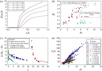
, figure 2(a) shows examples of the shapes of granular jump profiles evolving with the Froude number, as measured in the laboratory by Faug et al. (Reference Faug, Childs, Wyburn and Einav2015).
(a) Examples of normalized granular jump profiles showing a transition from diffuse to steep jumps, from Faug et al. (Reference Faug, Childs, Wyburn and Einav2015). (b,c,d) Comparison of parameters that play a role in (2.23) or (2.10): (b)
 $K_{0}$
versus
 $Fr$
; (c)
 $L/(h_{\ast }-h)$
versus
 $\unicode[STIX]{x1D701}$
; (d)
 $L/h$
versus
 $Fr$
. The following conditions are considered: water flows down inclined channels (data from Ohtsu & Yasuda (Reference Ohtsu and Yasuda1991), Husain et al. (Reference Husain, Alhamid and Negm1994)), water flows on rough beds (data from Hughes & Flack (Reference Hughes and Flack1984), Carollo et al. (Reference Carollo, Ferro and Pampalone2007)) and flows of dry granular material (data by Faug et al. (Reference Faug, Childs, Wyburn and Einav2015)). It should be noted that in (c), the data by Carollo et al. (Reference Carollo, Ferro and Pampalone2007) are below all other data with water because here the length of the roller,
 $L_{r}$
, was measured instead of the jump length (see figure 1(a) and text for explanation). For
 $\unicode[STIX]{x1D701}=0$
, a great number of tests were conducted, and the data showed a scatter related to some effect of
 $Fr$
(c); we then show a larger symbol that corresponds to the average value.

3.2 Variation of the shape factor
 $K_{0}$

The shape factor
 $K_{0}$
, defined by (2.5), is useful for estimation of the averaged value over the jump length of physical quantities (see, for instance, the estimation of
 $u_{J}$
) that depend on the position within the jump. The shape factor was only measured by Ohtsu & Yasuda (Reference Ohtsu and Yasuda1991) and Husain et al. (Reference Husain, Alhamid and Negm1994) for hydraulic jumps, and by Faug et al. (Reference Faug, Childs, Wyburn and Einav2015) for granular jumps. Figure 2(b) shows how the shape factor
 $K_{0}$
measured in the aforementioned studies varies with the Froude number
 $Fr$
of the incoming flow. Data by Husain et al. (Reference Husain, Alhamid and Negm1994) for water and by Faug et al. (Reference Faug, Childs, Wyburn and Einav2015) for granular fluids are remarkably of the same order of magnitude. Both data sets show that
 $K_{0}$
increases with
 $Fr$
. This trend was, however, not observed by Ohtsu & Yasuda (Reference Ohtsu and Yasuda1991), who found a nearly constant
 $K_{0}$
(equal to
 $1$
) in their experiments with water, although the range of
 $Fr$
that they investigated was similar. It should be noted that a slight decrease of
 $K_{0}$
with slope was observed by Ohtsu & Yasuda (Reference Ohtsu and Yasuda1991). However, this decrease was not observed by Husain et al. (Reference Husain, Alhamid and Negm1994). In the present paper (see § 4), we will consider
 $K_{0}=1$
for other experimental studies for which
 $K_{0}$
was not directly measured or estimated; this concerns the data by Peterka (Reference Peterka1984) for water jumps down a smooth incline and by Hughes & Flack (Reference Hughes and Flack1984) and Carollo et al. (Reference Carollo, Ferro and Pampalone2007) for water jumps on a rough bed.
3.3 Variation of the relative length
$L/(h_{\ast }-h)$

The relative length
 $L/(h_{\ast }-h)$
, which appears in the simplified implicit relation (2.10) derived from the assumption
 $\unicode[STIX]{x1D70C}_{\ast }/\unicode[STIX]{x1D70C}=1$
in the case of granular jumps, is analysed here. With both grains and water,
 $L/(h_{\ast }-h)$
is a decreasing function of the slope, as shown in figure 2(c). It is worth noticing that
 $L/(h_{\ast }-h)$
reaches a finite value of around
 $6{-}8$
for water flows at
 $\unicode[STIX]{x1D701}=0$
, as shown in figure 2(c). Such a range is consistent with values reported by a number of earlier studies, as for instance in Riegel & Beebe (Reference Riegel and Beebe1917) and Bakhmeteff & Matzke (Reference Bakhmeteff and Matzke1936). For valuable reviews that summarize the great number of experimental data sets on the length of hydraulic jumps, one can mention the works by Hager (Reference Hager1992) and, more recently, Schulz et al. (Reference Schulz, Nóbrega, Simões, Schulz and de Melo Porto2015). It should be noted that in the paper of Carollo et al. (Reference Carollo, Ferro and Pampalone2007), it was not the total length of the jump
 $L$
but the length of the roller
 $L_{r}$
that was measured (see the sketch in figure 1
a). However, the sequent depth was not measured at the end of the roller but – like in the other papers – at the end of the jump. Strictly, (2.23) should apply to
 $L$
and
 $h_{\ast }$
or to
 $L_{r}$
and the flow height at the end of the roller, but should not apply to
 $L_{r}$
and
 $h_{\ast }$
. The length of the roller is generally smaller than the length of the jump and approaches the latter when the Froude number increases, as reported by Rajaratnam (Reference Rajaratnam1967). Such a difference between
 $L$
and
 $L_{r}$
becomes clear at
 $\unicode[STIX]{x1D701}=0$
and
 $r=0$
. For a horizontal smooth bed,
 $L/(h_{\ast }-h)$
is around
 $7$
(data of Hughes & Flack (Reference Hughes and Flack1984), Peterka (Reference Peterka1984) and Husain et al. (Reference Husain, Alhamid and Negm1994) shown by yellow points in figure 2
c), while
 $L_{r}/(h_{\ast }-h)$
is around
 $4$
(data of Carollo et al. (Reference Carollo, Ferro and Pampalone2007) shown by turquoise points in figure 2
c).
Steady granular flows can only occur above a slope angle
 $\unicode[STIX]{x1D701}_{0}$
, which was approximately
 $23^{\circ }$
in the laboratory test by Faug et al. (Reference Faug, Childs, Wyburn and Einav2015). No jump can form below this limit angle, and when
 $\unicode[STIX]{x1D701}\mapsto \unicode[STIX]{x1D701}_{0}$
, the relative length of the jump
 $L/(h_{\ast }-h)$
starts to diverge, as seen in figure 2(c). However, for higher values of
 $\unicode[STIX]{x1D701}$
, the values seem to align with the data with water. The Froude number of granular flows is mainly controlled by the slope angle, and decreases with the slope. In contrast, it is possible to form supercritical water flows at high
 $Fr$
(far above the critical Froude number) on low slope angles, which can then produce strong hydraulic jumps of finite length. On approaching the slope
 $\unicode[STIX]{x1D701}_{0}$
,
 $Fr$
tends towards the critical Froude number, meaning that simultaneously
 $h_{\ast }$
approaches
 $h$
: the jump is more and more diffuse and finally disappears, as observed by Faug et al. (Reference Faug, Childs, Wyburn and Einav2015). The behaviour of granular jumps close to
 $\unicode[STIX]{x1D701}_{0}$
needs further investigation.
3.4 Variation of the relative length
$L/h$

Figure 2(d) shows how the jump length relative to the height of the incoming flow evolves with the Froude number. The behaviour of the relative length of the jump,
 $L/h$
, changes strongly between dry granular flows and hydraulic flows. For granular jumps,
 $L/h$
is almost independent of
 $Fr$
, and relatively small (around
 $10{-}20$
in the tests by Faug et al. (Reference Faug, Childs, Wyburn and Einav2015)) in comparison with the value obtained with hydraulic jumps (from
 $10$
to
 $160$
). These results suggest that the friction between grains is able to dissipate the energy of the incoming flow efficiently over a relatively small distance.
On the contrary, figure 2(d) suggests that the relative length of the jump
 $L/h$
is highly correlated with the Froude number in hydraulic flows, whether the channel is inclined or horizontal, smooth or rough. At a given
 $Fr$
, it is clear from figure 2(d) that the relative length of the jump is smaller if the bottom is rough, and it decreases as the typical roughness size increases. This means that a rough channel bottom is more able to dissipate energy than a smooth one. This result shows the key role played by the friction forces acting within the jump volume, thus justifying the general jump relation that we are proposing here.
Interestingly, the slope has no effect on the relative length
 $L/h$
of the jumps formed on a smooth bottom: the blue points for the jumps in water flows down a smooth incline and the yellow points for the jumps in water flows on a horizontal smooth bottom are aligned in figure 2(d). This means that at a given
 $Fr$
, the jump length is only proportional to the height of the incoming flow and does not depend on the slope angle. We will propose simple closure relations for
 $L/h$
in § 4.4.
3.5 Depth-averaged friction laws derived using minimal assumptions
Determination of the dimensionless number
 $\unicode[STIX]{x1D6E4}_{e}$
, namely the effective friction coefficient
 $\unicode[STIX]{x1D707}_{e}$
within the granular jump or the hydraulic friction coefficient
 $f_{e}$
within the hydraulic jump, is of course a very challenging question, linked to the rheology of the fluid at stake, the system size and/or the boundary conditions (bottom roughness in particular). We adopt here a back-analysis strategy. In the first step, we compute the exact values of
 $\unicode[STIX]{x1D6E4}_{e}$
needed to match (2.23) to the experimental data. In the second step, we compare these exact values with the predictions from friction laws derived using minimal assumptions under which the dimensionless number
 $\unicode[STIX]{x1D6E4}_{e}$
is a function of the incoming flow features. In the present section, we consider
 $\unicode[STIX]{x1D6FD}=\unicode[STIX]{x1D6FD}_{\ast }=1$
and
 $k=k_{\ast }=1$
in (2.23). These assumptions will be discussed in § 3.6.
3.5.1 Friction law for hydraulic flow on a rough bottom
Based on the phenomenological theory of Kolmogórov, Gioia & Chakraborty (Reference Gioia and Chakraborty2006) proposed to calculate the turbulent friction coefficient
 $f_{e}$
in rough pipes with the following formula:
 $$\begin{eqnarray}f_{e}=\unicode[STIX]{x1D705}_{\unicode[STIX]{x1D70F}}\unicode[STIX]{x1D705}_{u}\left(\frac{r}{R_{h}}+ab\Re ^{-3/4}\right)^{1/3},\end{eqnarray}$$
where
 $\unicode[STIX]{x1D705}_{\unicode[STIX]{x1D70F}}$
and
 $\unicode[STIX]{x1D705}_{u}$
are dimensionless numbers,
 $a$
and
 $b$
are constants (see more details in Gioia & Chakraborty (Reference Gioia and Chakraborty2006) for typical values for flows in rough pipes),
 $R_{h}$
is the hydraulic radius, which is equal to
 $(Wh)/(W+2h)\approx h$
for the free-surface flows investigated here,
 $r$
is the typical roughness size and
 $\Re =\bar{u}R_{h}/\unicode[STIX]{x1D708}\approx Fr\sqrt{g}h^{3/2}/\unicode[STIX]{x1D708}$
is the depth-averaged Reynolds number (
 $\unicode[STIX]{x1D708}$
being the fluid viscosity).
For the data revisited in the present study, the Reynolds number was always larger than
 $10^{7}$
. We can therefore neglect the influence of
 $\Re$
in (3.1) and express the dimensionless number
 $\unicode[STIX]{x1D6E4}_{e}$
(with
 $R_{h}\sim h$
) as
 $$\begin{eqnarray}\unicode[STIX]{x1D6E4}_{e}=\frac{1}{2}K_{0}\unicode[STIX]{x1D705}_{\unicode[STIX]{x1D70F}}\unicode[STIX]{x1D705}_{u}\left(\frac{r}{h}\right)^{1/3}Fr^{2}.\end{eqnarray}$$
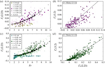
Figures 3(a) and 3(c) show the values of
 $\unicode[STIX]{x1D6E4}_{e}$
back-calculated from the general jump relation, namely (2.23), as a function of the Froude number for the data from Hughes & Flack (Reference Hughes and Flack1984) and Carollo et al. (Reference Carollo, Ferro and Pampalone2007) respectively. (For the data of Peterka (Reference Peterka1984), Ohtsu & Yasuda (Reference Ohtsu and Yasuda1991) and Husain et al. (Reference Husain, Alhamid and Negm1994), the bottom is smooth, then
 $r=0$
and
 $\unicode[STIX]{x1D6E4}_{e}=0$
.) At a given Froude number,
 $\unicode[STIX]{x1D6E4}_{e}$
is higher for higher
 $r$
, and, at a given
 $r$
,
 $\unicode[STIX]{x1D6E4}_{e}$
increases with
 $Fr$
. These trends are compatible with the friction law given by (3.2) (see the black circle symbols representing the turbulent friction law for some specific values of
 $r$
in figure 3
a,c). Figures 3(b) and 3(d) depict the best calibration of
 $\unicode[STIX]{x1D705}_{\unicode[STIX]{x1D70F}}\unicode[STIX]{x1D705}_{u}$
to fit the dimensionless number
 $\unicode[STIX]{x1D6E4}_{e}$
extracted from the hydraulic friction law (3.2) on the
 $\unicode[STIX]{x1D6E4}_{e}$
derived from the general jump relation (2.23) for the data from Hughes & Flack (Reference Hughes and Flack1984) and Carollo et al. (Reference Carollo, Ferro and Pampalone2007) respectively. Although some scatter is observed, the results of the calibration show that (3.2) is suitable for describing the value of
 $\unicode[STIX]{x1D6E4}_{e}$
within the jump provided that the product
 $\unicode[STIX]{x1D705}_{\unicode[STIX]{x1D70F}}\unicode[STIX]{x1D705}_{u}$
is taken equal to
 $0.0086$
for the data of Carollo et al. (Reference Carollo, Ferro and Pampalone2007) and equal to
 $0.0026$
for the data of Hughes & Flack (Reference Hughes and Flack1984). These two values of
 $\unicode[STIX]{x1D705}_{\unicode[STIX]{x1D70F}}\unicode[STIX]{x1D705}_{u}$
have the same order of magnitude, both leading to an
 $f_{e}$
compatible with typical values for hydraulic turbulent friction. A number of sources may explain the difference, however: some discrepancies in the geometry of the experimental set-up, some differences in the way of estimating
 $r$
in the two studies and, first of all, the fact that the calculated
 $\unicode[STIX]{x1D6E4}_{e}$
from the general jump relation in Carollo et al. (Reference Carollo, Ferro and Pampalone2007) uses the roller length
 $L_{r}$
instead of the jump length
 $L$
(see the previous discussion in § 3.3). Although the above questions remain open, (3.2) will be used in § 4 as a good approximation of basal effective friction within the water jump on a rough bottom.
Calibration of
 $\unicode[STIX]{x1D705}_{\unicode[STIX]{x1D70F}}\unicode[STIX]{x1D705}_{u}$
in the friction law given by (3.2) for water flows on a rough bed: (a)
 $\unicode[STIX]{x1D6E4}_{e}$
derived from the jump relation as a function of the Froude number for data from Hughes & Flack (Reference Hughes and Flack1984); (b) best match between
 $\unicode[STIX]{x1D6E4}_{e}$
calculated from (3.2) and
 $\unicode[STIX]{x1D6E4}_{e}$
back-calculated from the data and (2.23) obtained with
 $\unicode[STIX]{x1D705}_{\unicode[STIX]{x1D70F}}\unicode[STIX]{x1D705}_{u}=0.0026$
for data from Hughes & Flack (Reference Hughes and Flack1984); (c)
 $\unicode[STIX]{x1D6E4}_{e}$
derived from the jump relation as a function of the Froude number for data from Carollo et al. (Reference Carollo, Ferro and Pampalone2007); (d) best match between
 $\unicode[STIX]{x1D6E4}_{e}$
calculated from (3.2) and
 $\unicode[STIX]{x1D6E4}_{e}$
back-calculated from the data and (2.23) with
 $\unicode[STIX]{x1D705}_{\unicode[STIX]{x1D70F}}\unicode[STIX]{x1D705}_{u}=0.0086$
for data from Carollo et al. (Reference Carollo, Ferro and Pampalone2007) (calculation with
 $L_{r}$
). In (a) ((c) respectively), the black circle symbols depict a prediction from (3.2) with
 $r=0.64$
cm (
 $r=1.5$
cm respectively).

3.5.2 Friction law for granular flows
It is still a challenging question to predict accurately the friction law for granular flows down rough or smooth inclines, although many valuable studies have been conducted in recent years, as recently reviewed by Jop (Reference Jop2015) and references therein. In the present paper, we use a minimal assumption that the effective friction
 $\unicode[STIX]{x1D707}_{e}$
is given by the sum of a constant Coulombian-like friction coefficient, associated with the slope above which flows are possible, and a turbulent-like friction proportional to the square of the Froude number of the incoming flow, associated with the inertial forces that come into play at high
 $Fr$
,
 $$\begin{eqnarray}\unicode[STIX]{x1D707}_{e}=\unicode[STIX]{x1D707}_{s}+\unicode[STIX]{x1D6FC}Fr^{2},\end{eqnarray}$$
where
 $\unicode[STIX]{x1D707}_{s}$
and
 $\unicode[STIX]{x1D6FC}$
are the two parameters needed for the friction law. Such a law can be seen as a rough approximation of a number of granular flow models proposed in recent studies, and capable of covering a wide range of shallow flow conditions from dense inertial liquid flows to high-speed collisional gaseous flows (Louge & Keast Reference Louge and Keast2001; Berzi, di Prisco & Vescovi Reference Berzi, di Prisco and Vescovi2011; Holyoake & McElwaine Reference Holyoake and Mcelwaine2012).
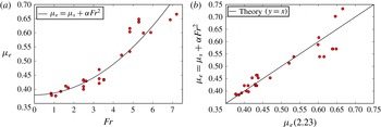
Calibration of
 $\unicode[STIX]{x1D707}_{s}$
and
 $\unicode[STIX]{x1D6FC}$
in the friction law given by (3.3) for dry granular flows: (a)
 $\unicode[STIX]{x1D707}_{e}$
derived from the jump relation as a function of the Froude number for data from Faug et al. (Reference Faug, Childs, Wyburn and Einav2015); (b) best match between
 $\unicode[STIX]{x1D707}_{e}$
calculated from (3.3) and
 $\unicode[STIX]{x1D707}_{e}$
back-calculated with the data and (2.23) obtained with
 $\unicode[STIX]{x1D6FC}=0.0068$
and
 $\unicode[STIX]{x1D707}_{s}=0.38$
for data from Faug et al. (Reference Faug, Childs, Wyburn and Einav2015).

Figure 4(a) shows the friction
 $\unicode[STIX]{x1D707}_{e}$
derived from the general jump relation, namely (2.23), as a function of the Froude number. We recall that
 $\unicode[STIX]{x1D707}_{e}$
corresponds to an effective coefficient of friction estimated over the entire length of the jump. The data are compatible with the friction granular law given by (3.3). We can match (3.3) to the experimental data on granular jumps down a smooth incline reported by Faug et al. (Reference Faug, Childs, Wyburn and Einav2015), and the best fit is found with
 $\unicode[STIX]{x1D707}_{s}=0.38$
and
 $\unicode[STIX]{x1D6FC}=0.0068$
. The value
 $\unicode[STIX]{x1D707}_{s}=0.38$
is equivalent to a friction angle of
 $20.8^{\circ }$
. The results are displayed in figure 4(b). It should be noted that if
 $\unicode[STIX]{x1D707}_{s}$
is estimated as equal to
 $\arctan (\unicode[STIX]{x1D701}_{0})$
, in accordance with
 $\unicode[STIX]{x1D701}_{0}=23^{\circ }$
as reported by Faug et al. (Reference Faug, Childs, Wyburn and Einav2015), it yields
 $\unicode[STIX]{x1D707}_{s}=\tan \unicode[STIX]{x1D701}_{0}=0.42$
and we obtain the best match between
 $\unicode[STIX]{x1D707}_{e}$
calculated with (3.3) and
 $\unicode[STIX]{x1D707}_{e}$
back-calculated by fitting the general jump relation (2.23) with
 $\unicode[STIX]{x1D6FC}=0.0053$
.
It should be noted that Faug et al. (Reference Faug, Childs, Wyburn and Einav2015) proposed a different analysis by considering a depth-averaged
 $\unicode[STIX]{x1D707}(I)$
rheology spatially integrated over the length of the jump. Their analysis was successful at demonstrating that the
 $\unicode[STIX]{x1D707}(I)$
rheology holds inside the volume of the jump. However, their approach was not predictive because
 $\unicode[STIX]{x1D707}_{e}$
was a function of the depth-averaged inertial number of the jump (averaged value over the length of the jump), which was by construction a function of the downstream jump features (
 $h_{\ast }$
,
 $\bar{u}_{\ast }$
and
 $\unicode[STIX]{x1D70C}_{\ast }$
) in addition to the upstream jump features. Moreover, their analysis was limited to non-accelerating flows for which flows were relatively dense, as detailed in Faug et al. (Reference Faug, Childs, Wyburn and Einav2015). Other laws exist to improve the
 $\unicode[STIX]{x1D707}(I)$
rheology, like the one proposed by Weinhart et al. (Reference Weinhart, Thornton, Luding and Bokhove2012), but they have many parameters and still do not take into account the inertia at high Froude numbers. In contrast, the more simple closure relation proposed here for friction, namely (3.3), can be predictive in the sense that we seek
 $\unicode[STIX]{x1D707}_{e}$
as a function of the incoming flow features only (
 $h$
and
 $\bar{u}$
). Moreover, it can be extended to fast accelerating and more dilute flows for which resistive forces proportional to
 $\bar{u}^{2}$
are no longer negligible.
3.6 Discussion on other parameters in the general jump relation:
$\unicode[STIX]{x1D70C}_{\ast }/\unicode[STIX]{x1D70C}$
,
$k$
,
$k_{\ast }$
,
$\unicode[STIX]{x1D6FD}$
and
$\unicode[STIX]{x1D6FD}_{\ast }$


When the fluid at stake is compressible, it is important to consider the change in density across the jump. Such an effect has recently been identified by Faug et al. (Reference Faug, Childs, Wyburn and Einav2015), who investigated standing jumps formed in dilute granular flows. Their study clearly showed the transition towards highly compressible jumps when the incoming granular flow became dilute. Not taking into account the change in density
 $\unicode[STIX]{x1D70C}_{\ast }/\unicode[STIX]{x1D70C}$
across the jump leads to a prediction that overestimates the jump height (see figure 10 in Faug et al. (Reference Faug, Childs, Wyburn and Einav2015)), itself being reduced by the energy dissipated (through collisions) to transit from a dilute supercritical flow to a much denser subcritical flow. It should be noted that
 $\unicode[STIX]{x1D70C}_{\ast }$
can be deduced from an assumption of random close packing for all slope angles because the flow after the jump is thick and very dense, but prediction of the decrease with slope of the density
 $\unicode[STIX]{x1D70C}$
of the incoming supercritical granular flow remains challenging.
In the present study, the parameters
 $k$
,
 $k_{\ast }$
,
 $\unicode[STIX]{x1D6FD}$
and
 $\unicode[STIX]{x1D6FD}_{\ast }$
were all taken equal to
 $1$
. This choice is strictly valid for fast hydraulic flows only.
The parameter
 $\unicode[STIX]{x1D6FD}$
is defined as the ratio between the depth-averaged value of the velocity squared and the square of the depth-averaged velocity:
 $\unicode[STIX]{x1D6FD}=\bar{u^{2}}/\bar{u}^{2}$
. It depends on the shape of the velocity profile:
 $\unicode[STIX]{x1D6FD}=1$
for plug flows,
 $\unicode[STIX]{x1D6FD}=4/3$
for a linear velocity profile and
 $\unicode[STIX]{x1D6FD}=5/4$
for a Bagnold velocity profile. Faug et al. (Reference Faug, Childs, Wyburn and Einav2015) reported sliding velocities at the base of their granular flows and Bagnold-like velocity profiles above it. The theoretical value of
 $\unicode[STIX]{x1D6FD}$
for such velocity profiles is given by the following relation:
 $$\begin{eqnarray}\unicode[STIX]{x1D6FD}=1+\frac{9}{100\displaystyle \frac{\unicode[STIX]{x1D6FF}}{\unicode[STIX]{x1D6FE}}+36},\end{eqnarray}$$
where
 $\unicode[STIX]{x1D6FF}=u_{b}^{2}+6/5A(\unicode[STIX]{x1D701})\sqrt{gd}(h/d)^{3/2}u_{b}$
and
 $\unicode[STIX]{x1D6FE}=A(\unicode[STIX]{x1D701})^{2}gd(h/d)^{3}$
. The sliding velocity
 $u_{b}$
is taken at the base of the flow,
 $d$
denotes the grain diameter and
 $A(\unicode[STIX]{x1D701})$
is the Bagnold constant which is a function of the slope angle. It should be noted that for any positively defined values for
 $\unicode[STIX]{x1D6FF}$
and
 $\unicode[STIX]{x1D6FE}$
in (3.4) above, the value of
 $\unicode[STIX]{x1D6FD}$
can only vary between
 $1$
and
 $1.25$
. Indeed, using the values measured by Faug et al. (Reference Faug, Childs, Wyburn and Einav2015) for
 $u_{b}$
and
 $A(\unicode[STIX]{x1D701})$
, we find
 $\unicode[STIX]{x1D6FD}$
varying from
 $1.04$
(at the highest
 $\unicode[STIX]{x1D701}$
) to
 $1.2$
(at the lowest
 $\unicode[STIX]{x1D701}$
). Taking
 $\unicode[STIX]{x1D6FD}=1$
for the incoming flows before the jumps is then reasonable for the highest slopes (high
 $Fr$
), while it is an underestimate at the lowest slopes (low
 $Fr$
). The velocity profiles downstream of the granular jump were not measured, thus preventing an estimation of
 $\unicode[STIX]{x1D6FD}_{\ast }$
. A recent study by Saingier, Deboeuf & Lagrée (Reference Saingier, Deboeuf and Lagrée2016) has shown the importance of accounting for the exact value of
 $\unicode[STIX]{x1D6FD}$
while deriving the rheology of dense granular flows down inclines. A similar approach will need to be conducted in the future to investigate how the relation proposed for jumps can be influenced by the values of
 $\unicode[STIX]{x1D6FD}$
and
 $\unicode[STIX]{x1D6FD}_{\ast }$
.
The coefficient
 $k$
relates the normal stresses
 $\unicode[STIX]{x1D70E}_{xx}$
and
 $\unicode[STIX]{x1D70E}_{zz}$
through the relation
 $\unicode[STIX]{x1D70E}_{xx}=k\unicode[STIX]{x1D70E}_{zz}$
. A number of studies consider
 $k=1$
for flows of dry granular flows, as described by – among other studies – Silbert et al. (Reference Silbert, Ertas, Grest, Halsey, Levine and Plimpton2001) and Pouliquen & Forterre (Reference Pouliquen and Forterre2002). Other studies propose to extend soil mechanics concepts to the dynamics of granular flows and calculate
 $k$
as an earth pressure coefficient, as reported, for instance, by Savage & Hutter (Reference Savage and Hutter1989). As discussed by Faug (Reference Faug2015), it is most likely that
 $k=1$
is relevant for the incoming steady uniform or slightly accelerating flow (before the jump), while
 $k_{\ast }$
might be different from
 $1$
in the decelerating flow after the jump. Extensive discrete element simulations on granular jumps, in light of the recent simulations on three-dimensional steady and uniform flows performed by Weinhart et al. (Reference Weinhart, Hartkamp, Thornton and Luding2013), are needed in the future in order to check the validity of this assumption.
4 General jump relation versus laboratory experiments
4.1 Hydraulic incompressible jump down a smooth incline:
$\unicode[STIX]{x1D6E4}_{e}=0$
,
$\unicode[STIX]{x1D70C}_{\ast }/\unicode[STIX]{x1D70C}=1$


We consider here hydraulic flows down smooth inclines. The standing jumps are then modelled by frictionless (
 $f_{e}=0$
, giving
 $\unicode[STIX]{x1D6E4}_{e}=0$
) and incompressible (
 $\unicode[STIX]{x1D70C}_{\ast }/\unicode[STIX]{x1D70C}=1$
) conditions. Because of the slope
 $\unicode[STIX]{x1D701}$
, we must take into account the component along the slope of the weight of the jump acting within the jump volume. This situation should be well described by (2.23) with
 $\unicode[STIX]{x1D70C}_{\ast }/\unicode[STIX]{x1D70C}=1$
and
 $\unicode[STIX]{x1D6E4}_{e}=0$
. Figure 5(a) depicts the sequent depth ratio as a function of the Froude number for different slope angles
 $\unicode[STIX]{x1D701}$
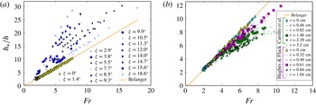
, as reported by Peterka (Reference Peterka1984), Ohtsu & Yasuda (Reference Ohtsu and Yasuda1991) and Husain et al. (Reference Husain, Alhamid and Negm1994). As expected, increasing the slope
 $\unicode[STIX]{x1D701}$
produces jumps thicker than those predicted by the Bélanger equation (line in figure 5(a)), and the gap increases with
 $\unicode[STIX]{x1D701}$
. By considering
 $\unicode[STIX]{x1D6E4}_{e}=0$
(
 $f_{e}=0$
),
 $\unicode[STIX]{x1D70C}_{\ast }/\unicode[STIX]{x1D70C}=1$
, the values actually measured in the experiments for
 $L/h$
and
 $K_{0}$
, and the input value of
 $\tan \unicode[STIX]{x1D701}$
, we verify that the jump height measured in the experiments can be predicted by (2.23) whatever the value of
 $\unicode[STIX]{x1D701}$
(see the blue diamond symbols in figure 7(a), which is provided in § 4.4).
Sequent depth ratio of standing water jumps, as a function of the Froude number, formed in hydraulic flows down smooth inclines, as reported by Peterka (Reference Peterka1984), Ohtsu & Yasuda (Reference Ohtsu and Yasuda1991) and Husain et al. (Reference Husain, Alhamid and Negm1994) (a), and in horizontal flows down a rough bottom, as reported by Hughes & Flack (Reference Hughes and Flack1984) and Carollo et al. (Reference Carollo, Ferro and Pampalone2007) (b). The continuous line depicts the prediction of the Bélanger equation in both panels.

4.2 Hydraulic incompressible jump on rough horizontal channel:
$\unicode[STIX]{x1D6E4}_{e}\neq 0$
,
$\unicode[STIX]{x1D70C}_{\ast }/\unicode[STIX]{x1D70C}=1$


In the situation analysed here, the fluid is still incompressible (
 $\unicode[STIX]{x1D70C}_{\ast }/\unicode[STIX]{x1D70C}=1$
), the slope is zero (
 $\tan \unicode[STIX]{x1D701}=0$
) but a turbulent friction between the fluid and the bed exists (
 $f_{e}\neq 0$
yields
 $\unicode[STIX]{x1D6E4}_{e}\neq 0$
) because of the presence of a rough bed, described by the roughness coefficient
 $r$
. When
 $r$
is null, the system is described by the Bélanger equation, and when it is not, (2.23) has to be used with
 $\unicode[STIX]{x1D70C}_{\ast }/\unicode[STIX]{x1D70C}=1$
and
 $\tan \unicode[STIX]{x1D701}=0$
. Figure 5(b) displays the sequent depth ratio as a function of the Froude number for different bed conditions, as reported by Hughes & Flack (Reference Hughes and Flack1984) and Carollo et al. (Reference Carollo, Ferro and Pampalone2007). As expected, increasing the bed roughness leads to jumps thinner than those predicted by the Bélanger equation (line in figure 5
b), and the gap between the experiments and the Bélanger equation increases with
 $r$
. Moreover, at a given
 $r$
, it is observed that the gap between the Bélanger equation and the experiments increases when
 $Fr$
increases. By considering
 $\tan \unicode[STIX]{x1D701}=0$
,
 $\unicode[STIX]{x1D70C}_{\ast }/\unicode[STIX]{x1D70C}=1$
, the values measured for
 $L/h$
and
 $K_{0}$
, and a
 $\unicode[STIX]{x1D6E4}_{e}$
that follows a turbulent friction law given by (3.2), we verify that the exact jump height can be predicted by (2.23) whatever the values of
 $r$
and
 $Fr$
(see the triangle symbols in green and magenta shown in figure 7(a), which is provided in § 4.4).
We have checked that use of the equation of degree four (see (2.14) in § 2.2) causes little change to the results displayed in figure 7(a), thus showing that the cubic equation is a good approximation for water jumps.
4.3 Granular compressible jump on a smooth incline:
$\unicode[STIX]{x1D707}_{e}\neq 0$
,
$\unicode[STIX]{x1D70C}_{\ast }/\unicode[STIX]{x1D70C}\neq 1$


For granular flows, all parameters of (2.23) come into play. Flows of granular materials are compressible (
 $\unicode[STIX]{x1D70C}_{\ast }/\unicode[STIX]{x1D70C}\neq 1$
) and frictional (
 $\unicode[STIX]{x1D6E4}_{e}=\unicode[STIX]{x1D707}_{e}\neq 0$
) flows, and they can occur only if the slope is greater than a limit angle (
 $\tan \unicode[STIX]{x1D701}>\tan \unicode[STIX]{x1D701}_{0}\neq 0$
). All of these effects are included in (2.23).
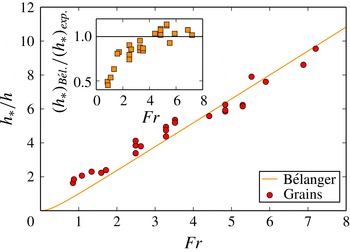
Sequent depth ratio for dry granular material flowing down an incline versus the Froude number (laboratory data reported by Faug et al. (Reference Faug, Childs, Wyburn and Einav2015)), compared with the Bélanger equation (continuous line). Inset: sequent depth ratio calculated with the Bélanger equation, scaled by the sequent depth ratio measured in the experiments by Faug et al. (Reference Faug, Childs, Wyburn and Einav2015).

Figure 6 shows the sequent depth ratio for standing jumps formed in granular material down an incline versus the Froude number, as reported by Faug et al. (Reference Faug, Childs, Wyburn and Einav2015). The Bélanger equation (line in figure 6) looks to predict quite well the sequent depth ratio of granular jumps at high Froude numbers, for which the effect of the difference between
 $\tan \unicode[STIX]{x1D701}$
and
 $\unicode[STIX]{x1D707}_{e}$
is relatively small, but this is not true for lower values of the Froude number. The prediction of the Bélanger equation becomes very poor at low
 $Fr$
, as shown in the inset of figure 6 which reports the values of
 $h_{\ast }/h$
predicted by the Bélanger equation (square symbols) versus the values of
 $h_{\ast }/h$
actually measured in the laboratory tests. By considering the values of
 $\unicode[STIX]{x1D70C}_{\ast }/\unicode[STIX]{x1D70C}$
,
 $L/h$
and
 $K_{0}$
measured by Faug et al. (Reference Faug, Childs, Wyburn and Einav2015), as well as the exact values of
 $\tan \unicode[STIX]{x1D701}$
, and a
 $\unicode[STIX]{x1D707}_{e}$
that follows the friction law given by (3.3), we verify that we can reproduce the heights of granular jumps measured in the laboratory (see the red-coloured circle symbols in figure 7
a) whatever the value of the Froude number of the incoming flow.
4.4 Analysing both water and granular fluids
Figure 7 displays the heights of the jumps predicted by the general relation proposed for jumps as a function of the heights of the jumps actually measured in both water and granular fluids.
4.4.1 Verification of calibration regarding the friction laws
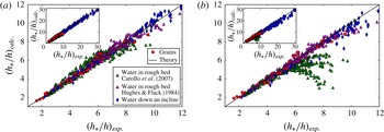
The collapse of the height of the jump shown in figure 7(a) is a verification of our calibration procedure regarding the friction laws. It was obtained by feeding the general solution, given by (2.23), with the values actually measured in the experiments for
 $K_{0}$
(or taken equal to
 $1$
when it was not known: Hughes & Flack (Reference Hughes and Flack1984), Peterka (Reference Peterka1984) and Carollo et al. (Reference Carollo, Ferro and Pampalone2007)),
 $L/h$
and
 $\unicode[STIX]{x1D70C}_{\ast }/\unicode[STIX]{x1D70C}$
(when the latter ratio was not
 $1$
: dilute granular flows), and by using minimal assumptions for the dimensionless number
 $\unicode[STIX]{x1D6E4}_{e}$
depending on the fluid and/or bottom roughness under consideration. The calibrated values used for
 $\unicode[STIX]{x1D705}_{\unicode[STIX]{x1D70F}}\unicode[STIX]{x1D705}_{u}$
for water, and
 $\unicode[STIX]{x1D707}_{s}$
and
 $\unicode[STIX]{x1D6FC}$
for dry grains, are given in §§ 3.5.1 and 3.5.2 respectively.
Sequent depth ratio calculated with (2.23) under minimal assumptions on closure relations for friction (when relevant: see text), versus the measured sequent depth ratio in experiments with water or dry grains: verification using the values of
 $L/h$
actually measured (a), and prediction using empirical but simple closure relations for
 $L/h$
depending on the fluid type (b). The insets show all the data available and revisited in the present paper, while the main panels are zooms on values of
 $h_{\ast }/h$
smaller than
 $12$
which correspond to a wide spectrum of fluid and boundary conditions.

4.4.2 Prediction using simple relations for
$L/h$
and
$K_{0}$


The general relation can predict the height of the jump only if another length scale, namely the jump length, is known. In order to make the general relation predictive, it is interesting to push forward our analysis by proposing an empirical law for
 $L/h$
instead of using the values actually measured in the laboratory experiments. In light of the variation of
 $L/h$
observed in the experiments (see figure 2
d), it appears to be reasonable to approximate the jump length by a linear function of the Froude number for the water flows:
 $$\begin{eqnarray}\frac{L}{h}=c(Fr-1),\end{eqnarray}$$
where
 $c$
takes the following values:
 $c=9.76$
for the smooth bottom,
 $c=7.71$
for the rough bottom in Hughes & Flack (Reference Hughes and Flack1984) and
 $c=4.54$
for the rough bottom in Carollo et al. (Reference Carollo, Ferro and Pampalone2007). It should be noted that the latter value is much lower because it is based on the roller length, which is smaller than the jump length. If we exclude the measurements that are based on the length of the roller, a reasonable value of
 $c$
to match the maximum of the measurements on the length of water jumps would be
 $8.7$
(mean value stemming from the data on a smooth bottom and the data on a rough bottom by Hughes & Flack (Reference Hughes and Flack1984)). The above law assumes that the jump length vanishes (
 $L=0$
) when
 $Fr$
reaches unity, which is the critical Froude number for water. Theoretical prediction of the length of the jump is still a question not resolved in hydraulics. There are a number of experimental studies on the length of hydraulic jumps, and a number of empirical laws have been proposed for
 $L/h$
, as reviewed by Hager (Reference Hager1992) and Schulz et al. (Reference Schulz, Nóbrega, Simões, Schulz and de Melo Porto2015). Equation (4.1) reproduces well the data shown in figure 2(d) and is similar to the equation proposed earlier by Silvester (Reference Silvester1964).
The relative jump length is – in strong contrast to water – nearly constant for dry granular flows (see the red circles in figure 2(d)). The mean value extracted from the data by Faug et al. (Reference Faug, Childs, Wyburn and Einav2015) is
 $$\begin{eqnarray}\frac{L}{h}\simeq 14.1,\end{eqnarray}$$
and the median value is
 $12.3$
. Figure 7(b) shows the height of the jump predicted by (2.23) fed with the above closure relations for
 $L/h$
(instead of using the measured values for
 $L/h$
), while keeping the calibrated parameters for the friction laws (values of
 $\unicode[STIX]{x1D705}_{\unicode[STIX]{x1D70F}}\unicode[STIX]{x1D705}_{u}$
for water flows on a rough bed, and of
 $\unicode[STIX]{x1D707}_{s}$
and
 $\unicode[STIX]{x1D6FC}$
for the dry granular flows, discussed in §§ 3.5.1 and 3.5.2 respectively). We use
 $L/h=14.1$
for grains and
 $L/h=c(Fr-1)$
, with
 $c=8.7$
, for water. In addition, we systematically consider
 $K_{0}=1$
. The collapse between the laboratory data and the analytical prediction remains very good for most of the data, which shows the robustness of the general relation proposed fed with simple closure relations for
 $\unicode[STIX]{x1D707}_{e}$
and
 $L/h$
. The high values of
 $h_{\ast }/h$
measured by Carollo et al. (Reference Carollo, Ferro and Pampalone2007) are discarded from the analytical prediction in figure 7(b) because they correspond to conditions for which the gap between
 $L_{r}$
(the roller length) and
 $L$
(the jump length) is the largest.
5 Discussion and conclusion
The present paper presented a general explicit relation for the prediction of the sequent depth ratio (
 $h_{\ast }/h$
) of standing jumps formed in free-surface flows, which was derived from depth-averaged mass and momentum conservation applied to the control volume surrounding the jump. We obtained a cubic equation for grains and an equation of degree four for water. The latter can be approximated by a cubic equation, as long as we have
 $h_{\ast }/h$
much greater than
 $1$
. The cubic equation, which is exact for grains and a reasonable approximation for water, could be solved by Cardano’s method. By revisiting different laboratory configurations involving (i) water flows on horizontal smooth beds or down smooth inclines, (ii) water flows on horizontal rough beds and (iii) dense and dilute flows of dry granular material down smooth inclines we were able to clearly delineate the importance of each contribution to the height of the standing jumps, as fully predicted by the general relation proposed. Our study demonstrates that this general relation is robust for a wide range of experimental conditions in the laboratory. The sequent depth ratio of the standing jump is not a function of the Froude number only. This clearly shows the limits of the traditional Bélanger equation which stems from a Rankine–Hugoniot relation and assumes – by construction – that the jump volume shrinks into a singular surface. The sequent depth of the jump is a function of the slope inclination: at a given
 $Fr$
, water jumps formed down a smooth incline are thicker than those formed on a horizontal smooth bed, which highlights the crucial role played by the component of the jump weight along the slope (figure 5
a). It is also a function of the resistive friction force: at a given
 $Fr$
, horizontal water jumps formed on a rough bed are thinner than those formed on a smooth bed, because energy is dissipated by friction (figure 5
b). At low
 $Fr$
, the standing jumps formed in dense flows of dry granular materials are thicker than those predicted by the Bélanger equation (see the inset of figure 6), because the contribution due to the jump weight reduced by the granular friction force (apparent weight along the slope) comes into play. At higher
 $Fr$
, the latter contribution of the apparent weight of the jump – which tends to increase the jump height – is counterbalanced by the decrease in density across the jump – which tends to decrease the jump height. This competition explains why standing jumps formed in fast dilute flows of dry granular material remain, however, well predicted by the traditional Bélanger equation (high
 $Fr$
in inset of figure 6), as observed by earlier studies (Brennen, Sieck & Paslaski Reference Brennen, Sieck and Paslaski1983; Gray, Tai & Noelle Reference Gray, Tai and Noelle2003).
In order to take into account the forces acting within the jump volume, it is necessary to feed the new general relation with the relative jump length (
 $L/h$
) and with information on its shape (
 $K_{0}$
), as well as with a closure relation for the friction force. In the present paper, we cross-compared the existing laboratory data to derive simple yet relevant closure relations for the friction laws, as discussed in §§ 3.5.1 and 3.5.2. Returning to figure 2(d), the variation of
 $L/h$
as a function of the experimental configuration (boundary conditions, rheology of the fluid at stake) is quite complicated. The relative jump length
 $L/h$
appears to depend weakly on
 $Fr$
for dry granular materials, while it increases (roughly) linearly with
 $Fr$
for water, but the increase rate with
 $Fr$
depends on the bottom roughness. As a conclusion to our study, it appears to be crucial to devote future research to the length of the standing normal jump and, to a lesser extent, the shape of the jump. Understanding how the geometry of the standing jump varies with the boundary conditions, the system size and the nature of the fluid in consideration, and thus how it is coupled with the basal effective friction, appears to be a promising approach to further understand the rheology of complex fluids such as granular flows. Future work should systematically investigate the assumption of decoupling the jump length,
 $L/h$
, and the parameters that characterize the dimensionless number
 $\unicode[STIX]{x1D6E4}_{e}$
(namely
 $\unicode[STIX]{x1D707}_{s}$
and
 $\unicode[STIX]{x1D6FC}$
for grains, and
 $f_{e}$
for water). Regarding the theoretical aspects presented in the current paper, it is worthwhile to note that derivation of an equation for energy conservation – in addition to mass and momentum conservation – would open a path to predict the geometry of the jump (size and shape), but this remains a challenging issue.
Acknowledgements
The authors are grateful to the Labex Tec21, which is part of the ANR ‘Investissements d’avenir’ programme, for funding. T.F. is grateful for the financial support by the People Programme (Marie Curie Actions) of the European Unions Seventh Framework Programme under REA Grant Agreement No. 622899 (FP7-PEOPLE-2013-IOF, GRAINPACT). I.E. is grateful for the support of the Australian Research Council through grant DP160104310. The authors would like to thank G. Chambon for the fruitful discussion they had with him on some theoretical aspects of the present study, as well as three anonymous referees for their insightful comments and suggestions on this paper.