1. Introduction
The transition from drag to thrust or Bénard–von Kármán (BvK) to reverse Bénard–von Kármán (rBvK) vortex street patterns for flapping foils has received renewed interest in recent two decades (see, for example, Godoy-Diana, Aider & Wesfreid Reference Godoy-Diana, Aider and Wesfreid2008; Bohl & Koochesfahani Reference Bohl and Koochesfahani2009; Schnipper, Andersen & Bohr Reference Schnipper, Andersen and Bohr2009; Mackowski & Williamson Reference Mackowski and Williamson2015; Andersen et al. Reference Andersen, Bohr, Schnipper and Walther2017; Kim & Lee Reference Kim and Lee2019; Lagopoulos, Weymouth & Ganapathisubramani Reference Lagopoulos, Weymouth and Ganapathisubramani2019; Tzezana & Breuer Reference Tzezana and Breuer2019, and references therein). The early studies (for example, Koochesfahani Reference Koochesfahani1989; Triantafyllou, Triantafyllou & Grosenbaugh Reference Triantafyllou, Triantafyllou and Grosenbaugh1993; Jones, Dohring & Platzer Reference Jones, Dohring and Platzer1998, and references therein) triggered the interest in understanding the structure and dynamics of the wakes created by flapping foils and their relation to thrust generation. The important non-dimensional parameter governing the force and the wake transitions is the Strouhal number (Triantafyllou, Triantafyllou & Gopalkrishnan Reference Triantafyllou, Triantafyllou and Grosenbaugh1991), defined as
 ${\textit{St}} = 2A f / U_{\infty }$
, where,
 $2A$
is the tip-to-tip amplitude of the trailing edge excursion of the flapping foil,
 $f$
is the flapping frequency and
 $U_{\infty }$
is the free-stream velocity. The change in the relative position of counterrotating vortices generated by a flapping foil with an increase in the Strouhal number (
 ${\textit{St}}$
) determines the wake transition and, eventually, the drag–thrust transition (Godoy-Diana et al. Reference Godoy-Diana, Aider and Wesfreid2008). For a flapping rigid foil, with increasing
 ${\textit{St}}$
, the usual route of wake transition is: BvK (momentum deficit, drag) to inline or neutral, in which the vortices with an alternating sense of rotation are arranged one behind the other in a line (momentumless wake, no drag or thrust), to rBvK (momentum excess, thrust). Force and flow measurements further revealed that the actual drag-to-thrust transition is followed by the BvK to rBvK transition of the vortex street (Bohl & Koochesfahani Reference Bohl and Koochesfahani2009; Mackowski & Williamson Reference Mackowski and Williamson2015). The effects of the flapping kinematics on the vortex wake and drag–thrust transition are also investigated in detail (Koochesfahani Reference Koochesfahani1989; Muijres & Lentink Reference Muijres and Lentink2007; Andersen et al. Reference Andersen, Bohr, Schnipper and Walther2017).
The transition to rBvK vortex street occurs beyond
 ${\textit{St}} \sim 0.18$
(Godoy-Diana et al. Reference Godoy-Diana, Aider and Wesfreid2008; Schnipper et al. Reference Schnipper, Andersen and Bohr2009). Further increase in
 ${\textit{St}}$
(
 $\gtrsim 0.35$
) breaks symmetry and produces a deflected (Godoy-Diana et al. Reference Godoy-Diana, Marais, Aider and Wesfreid2009) and meandering jet (Shinde & Arakeri Reference Shinde and Arakeri2013). However, the experiments by Marais et al. (Reference Marais, Thiria, Wesfreid and Godoy-Diana2012) showed that, by introducing flexibility to foil, the jet deflection can be suppressed for higher Strouhal numbers. They showed that the flexibility in the foil brings a stabilising effect to the wake by increasing the separation between the shed vortices and, effectively, preventing the vortex dipole formation that serves as a key to the jet deflection (Godoy-Diana et al. Reference Godoy-Diana, Marais, Aider and Wesfreid2009). Numerical investigation on a self-propelled plunging flexible foil by Zhu, He & Zhang (Reference Zhu, He and Zhang2014) showed that foil flexibility can either prevent or excite the symmetry breaking of the wake by modifying the vortex circulation. The experiments by Shinde & Arakeri (Reference Shinde and Arakeri2014) considered a case of zero free-stream velocity and showed that the flexibility in flapping foil suppresses the deflection as well as the meandering of the jet in the limiting case of
 ${\textit{St}} \rightarrow \infty$
, and the flexible foil generates a narrow, coherent jet aligned along the centreline. The mechanisms of jet meandering suppression and the details of the flow physics are elaborated in Shinde & Arakeri (Reference Shinde and Arakeri2014, Reference Shinde and Arakeri2018). Simulations on a heaving rigid foil with flexible aft tail by Shah et al. (Reference Shah, Majumdar, Bose and Sarkar2022) also showed how chordwise flexibility suppresses the jet switching and reinstates the wake periodicity. These recent studies have unravelled the prominent effect of foil flexibility on the generation and regulation of the wake structures, vortex street patterns and forces. It is necessary to understand how flexibility in flapping foils alters the wake-transition patterns.
The phase maps based on the Strouhal number (
 ${\textit{St}}$
) for the wake transitions for rigid flapping foils are well established (e.g. Godoy-Diana et al. Reference Godoy-Diana, Aider and Wesfreid2008; Schnipper et al. Reference Schnipper, Andersen and Bohr2009; Andersen et al. Reference Andersen, Bohr, Schnipper and Walther2017; Kim & Lee Reference Kim and Lee2019). Natural flapping foils (tails and fins in fish; wings in insects and birds), on the other hand, are usually flexible, completely or partially (Wootton Reference Wootton1999; Daniel & Combes Reference Daniel and Combes2002). Therefore, in addition to
 ${\textit{St}}$
, the flexural rigidity (
 ${\textit{EI}}$
;
 $E$
is Young’s modulus,
 $I$
is moment of inertia) of the flapping foil is expected to play an important role in determining the wake transitions. However, the question of how flexibility alters the transition criteria, vortex interactions and phase maps has not yet been explored experimentally. Although the interactions of fluid and flapping flexible foils are intricate and challenging, it is immensely important to understand the role of flexibility in flapping foils in wake transitions, and in enhancing thrust, lift and efficiency because of their increased usage in bioinspired propulsors like robotic fishes, insects, birds, autonomous underwater vehicles, micro aerial vehicles, etc. (Shyy, Berg & Ljungqvist Reference Shyy, Berg and Ljungqvist1999; Young et al. Reference Young, Walker, Richard, Taylor and Thomas2009; Lauder Reference Lauder2015; Quinn & Lauder Reference Quinn and Lauder2021). Therefore, understanding the role of flexibility on the wake-transition phase map and vortex interactions is imperative.
The numerical investigation by Kim & Lee (Reference Kim and Lee2019) for a heaving flexible foil explored the effects of flexibility by considering a single bending rigidity value on the transition boundaries and structures of the wake and thrust generation. They found that the circulations around the leading edge vortices (which are prominently generated during heaving motion) and trailing edge vortices play crucial roles in determining the wake transition and thrust attenuation. As the flexural rigidity of the natural flapping foil in fish, birds and insects varies over a wide range (Daniel & Combes Reference Daniel and Combes2002; Mountcastle & Daniel Reference Mountcastle and Daniel2009; Quinn & Lauder Reference Quinn and Lauder2021), it would be worth understanding how the variation in stiffness of the foil affects the structures and transitions in the wake of a flapping foil, and that yet remains to be unexplored.
We experimentally investigate the influence of flexibility of the foil pitching in a uniform planar two-dimensional (2-D) flow in a soap film at a low Reynolds number (
 ${\textit{Re}}$
) on vortex interactions and wake transitions. The use of planar soap films to investigate flapping foils and filaments is well established (Zhang et al. Reference Zhang, Childress, Libchaber and Shelley2000; Muijres & Lentink Reference Muijres and Lentink2007; Jia & Yin Reference Jia and Yin2008; Schnipper et al. Reference Schnipper, Andersen and Bohr2009; Andersen et al. Reference Andersen, Bohr, Schnipper and Walther2017). We analyse the interactions of vortices travelling over continuously deforming filaments and identify vortex interaction mechanisms (VIMs). By spanning flexural rigidity over three orders, we construct the
 ${\textit{St}}$
–
 ${\textit{EI}}$
phase maps for the wake transitions and the VIMs, perhaps for the first time.
2. Experiments
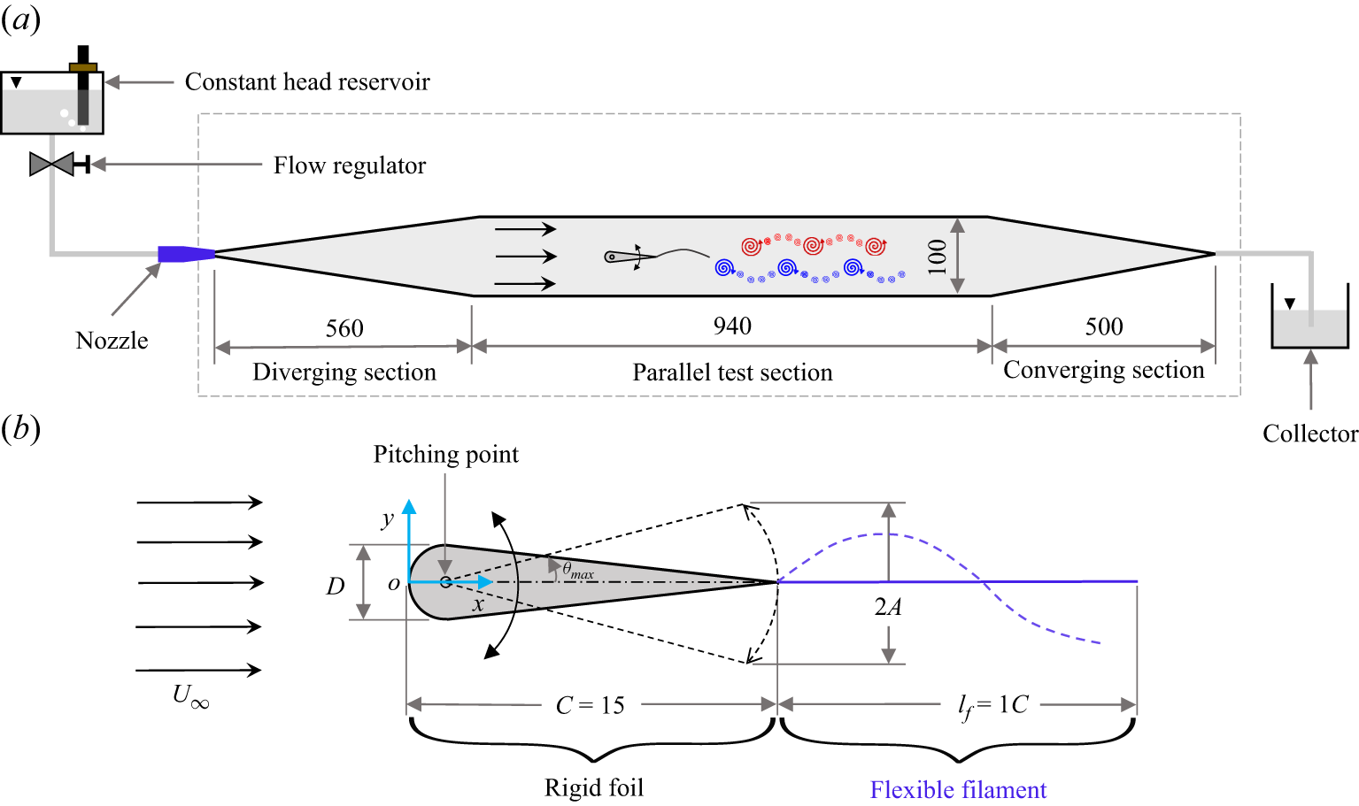
We conducted experiments in 2-D planar flow created using a gravity-driven inclined soap film tunnel (SFT); figure 1(a) provides the dimensional details. In our SFT, a soap solution, that contains
 $2\,\,\%$
dish-washing liquid (Dettol) by volume with
 $98\,\%$
reverse osmosis treated water, flows between two nylon guide wires (
 $0.7$
mm diameter) to create a film of thickness
 ${\sim} 4$
 $\unicode{x03BC}$
m and width of 100 mm. The constant pressure head at the flow-controlling rotameter valve is ensured by using Mariotte’s bottle mechanism in the soap solution reservoir. The soap film has a uniform velocity profile with an average free-stream velocity
 $U_{\infty }$
= 0.66 ms−1 that is kept constant to within 5 %; velocity is measured using tiny bubbles flowing in the film, similar to Schnipper et al. (Reference Schnipper, Andersen and Bohr2009). Finding the kinematic viscosity (
 $\nu$
) of the soap film is not straightforward, as it depends on the thickness of the flowing film. However, following the method of Vorobieff & Ecke (Reference Vorobieff and Ecke1999), we measured the vortex shedding frequency behind stationary circular cylinders (0.5, 1, 1.5, 2, 4, 6, 8 mm diameter) and using the well-studied
 ${\textit{St}}$
–
 ${\textit{Re}}$
relationship (Georgiev & Vorobieff Reference Georgiev and Vorobieff2002; Roushan & Wu Reference Roushan and Wu2005), we estimated
 $\nu$
= 5
 $\times$
10
 $^{-6}$
m
 $^2$
s−1.
Experimental details. (a) Schematic of SFT. The tunnel portion marked in a broken rectangle shows the top view. (b) Cross-section of flexible foil. The origin is at the leading edge (LE) at zero angle of attack. All dimensions are in mm.

The model (figure 1
b), referred to as ‘flexible foil’, consists of a symmetric rigid airfoil and a flexible filament. To impart the flapping motion to the flexible filament and to hold it in the flow, the flexible filament is attached to the trailing edge of the rigid foil. Manufactured using resin 3D printing, the rigid foil (chord,
 $C = 15$
mm) has a semicircular leading edge (LE,
 $D$
= 2.5 mm, maximum thickness) and two straight portions that join at the trailing edge (TE), forming a sharp tip. The chord to maximum thickness ratio (
 $C/D$
) is 6; note that we maintain the same
 $C/D$
ratio as that for the foil used by Schnipper et al. (Reference Schnipper, Andersen and Bohr2009). The foil ensures smooth flow over it. Our leading rigid foil is similar to that used in earlier studies on wake transition, for example, Heathcote & Gursul (Reference Heathcote and Gursul2007), Godoy-Diana et al. (Reference Godoy-Diana, Aider and Wesfreid2008), Schnipper et al. (Reference Schnipper, Andersen and Bohr2009), Andersen et al. (Reference Andersen, Bohr, Schnipper and Walther2017) and Van Buren, Floryan & Smits (Reference Van Buren, Floryan and Smits2019). As long as the foil is aerodynamic, moderately thick and symmetric, the leading rigid foil type will not significantly alter the flow. A lightweight, non-wetting, flexible filament (length,
 $l_{{\kern-1pt}f} = 1C$
) is attached to the TE. The flexural rigidity (
 ${\textit{EI}}$
) of the flexible filament is calculated by following the cantilever method suggested by DaDeppo & Schmidt (Reference DaDeppo and Schmidt1971) wherein the filament is treated as a cantilever beam fixed at one end and its slope at the deflected free end of filament tip (calculated based on measured filament tip deflection) is used to calculate the
 ${\textit{EI}}$
values; more details of the method can be found in DaDeppo & Schmidt (Reference DaDeppo and Schmidt1971). This method has been used earlier; see, for example, Ait Abderrahmane et al. (Reference Ait Abderrahmane, Paidoussis, Fayed and Ng2011) and Feng et al. (Reference Feng, Chen, Huang and Zhou2019).
The flexible foil is pierced perpendicularly into the film in the SFT test section. The sinusoidal pitching motion to the flexible foil is provided by a DC motor (RS-775) in combination with a solid-state relay and Arduino (UNO, Microcontroller: ATmega328) using a crank and slotted lever mechanism. The pitching point is at 1.25 mm from the LE; pitching amplitude is
 $\theta _{\textit{max}} = \pm 6^{\circ }$
, giving a peak-to-peak amplitude of
 $2A \simeq 2.87$
mm. The pitch-point location, pitching amplitude, filament length, free-stream velocity and Reynolds number (
 ${\textit{Re}}$
) are kept constant in our experiments.
The Reynolds number defined using the maximum thickness (
 $D$
) of the airfoil is
 ${\textit{Re}} = U_{\infty } D / \nu = 330$
. The Reynolds number based on chord as the length scale is
 ${\textit{Re}}_C = U_{\infty } C / \nu = 1980$
. The Reynolds number used in our experiments is comparable to that used in earlier studies on wake transition, for example, Godoy-Diana et al. (Reference Godoy-Diana, Aider and Wesfreid2008), Schnipper et al. (Reference Schnipper, Andersen and Bohr2009), Marais et al. (Reference Marais, Thiria, Wesfreid and Godoy-Diana2012), Zhu et al. (Reference Zhu, He and Zhang2014), Andersen et al. (Reference Andersen, Bohr, Schnipper and Walther2017) and Kim & Lee (Reference Kim and Lee2019). Moreover, this Reynolds number is well within the
 $10 \lt Re_C \lt 10^4$
range of ‘intermediate Reynolds numbers’ which characterise flapping-based propulsion in nature (Wang Reference Wang2005). Although the Reynolds number is fixed in our study, we vary two other important parameters in this intricate and inherently coupled fluid–structure interaction problem, viz., the Strouhal number (
 ${\textit{St}}$
), and the flexural rigidity (
 ${\textit{EI}}$
). The Strouhal number (
 ${\textit{St}} = 2A f / U_{\infty }$
) is varied via the pitching frequency (
 $f$
= 21–54 Hz). The Strouhal number range covered in our experiments is
 $0.084 \leqslant {\textit{St}} \leqslant 0.245$
. We varied the flexural rigidity (
 ${\textit{EI}}$
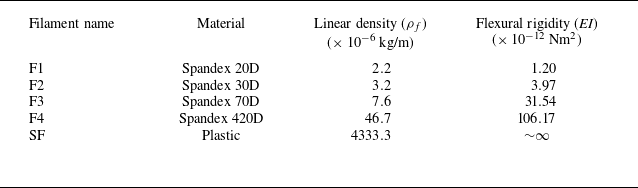
) of the flexible filament by three orders of magnitude using four Spandex filaments (F1, F2, F3, F4). Table 1 provides the properties of the filaments. We also explored two extreme cases: foil with no filament (NF), and foil with non-deformable solid filament (SF) to investigate the limiting case of
 ${\textit{EI}} \rightarrow \infty$
. We investigated a total of 90 cases ((4
 ${\textit{EI}}$
s + 1 NF + 1 SF)
 $\times$
15
 $f$
s).
Filament details.

The hydrodynamics of a soap film has been well studied, and the use of SFTs as a simple and elegant tool for flow visualisations, especially for various types of vortex-dominated flows, is well established (Couder & Basdevant Reference Couder and Basdevant1986; Gharib & Derango Reference Gharib and Derango1989; Rutgers et al. Reference Rutgers, Wu, Bhagavatula, Petersen and Goldburg1996; Beizaie & Gharib Reference Beizaie and Gharib1997; Rivera, Vorobieff & Ecke Reference Rivera, Vorobieff and Ecke1998; Zhang et al. Reference Zhang, Childress, Libchaber and Shelley2000; Rutgers, Wu & Daniel Reference Rutgers, Wu and Daniel2001). The flow speed in our experiments (0.66 m s−1) is significantly lower than the elastic longitudinal Marangoni wave speed in our soap film (
 ${\sim} 6.2$
m s−1); therefore, compressibility effects can be neglected, and the soap film can be treated as a 2-D incompressible fluid (Couder, Chomaz & Rabaud Reference Couder, Chomaz and Rabaud1989; Chomaz & Cathalau Reference Chomaz and Cathalau1990). As the film thickness variations are strongly coupled with vorticity (Rivera et al. Reference Rivera, Vorobieff and Ecke1998), the vortical flow structures emerging from the interaction of flexible foil with soap film are visualised using the well-established thin film interferometry technique (Couder et al. Reference Couder, Chomaz and Rabaud1989; Schnipper Reference Schnipper2011; Newburgh & Goodale Reference Newburgh and Goodale2009; Drake, Epperson & Burks Reference Drake, Epperson and Burks2020). In this technique, the light rays reflected from the top and bottom surfaces of the film interact to produce interference patterns. The nature of the interference pattern (constructive or destructive) is determined by the phase difference between the rays, which depends on the path travelled and, thus, on the film thickness. Bright and dark spots form, respectively, at the places of constructive and destructive interference. To illuminate the flow, we used a low-pressure sodium vapour lamp (GE-SOX-55W), which is a monochromatic light source. The vortical flow is captured at 1000 frames per second using a Photron FASTCAM Mini UX50 high-speed camera (1280
 $\times$
1024 pixels resolution).
3. Generation and interaction mechanisms of vortices
A flexible foil pitching in uniform flow generates a pair of big counter-rotating vortices along with multiple small vortices per cycle, which we term respectively as ‘primary vortices’ (PVs) and ‘secondary vortices’ (SVs) (see figure 2 a). To aid in identifying the VIMs, we classify the vortices rolling over a flexible foil as ‘boundary layer vortices’ (BLVs) and ‘trailing edge vortices’ (TEVs), as identified in figure 2(b). The genesis of BLV begins just downstream of the pitch point; it gathers vorticity from the foil boundary layer, grows and rolls over the foil (figure 2 b). When the TE crosses the centreline (CL), its velocity is maximum, and the filament deforms in such a way that it obstructs the fluid coming from the upper surface of the foil and leads to flow separation at the TE that results in the formation of a TEV; another TEV forms during the subsequent half-cycle by the same mechanism, from the fluid on the lower side of the foil. Three prominent wake patterns (viz., inline, BvK, rBvK) are shown in figure 3.
Wake of pitching flexible foil. (a) Vortices enclosed in big and small circles are, respectively, PVs and SVs. (b) Red and yellow curves enclose, respectively, BLVs and the TEV. Foil pitches symmetrically about the white CL. Note: because the camera is slightly inclined to the film, a small spanwise portion of foil is seen, hence the foil section does not appear symmetric about the CL. The greyish-white rectangle seen behind the foil is the base that holds the foil assembly.

Vortex street patterns behind a flexible foil (F2), identified based on relative positions of the PVs: (a) inline,
 ${\textit{St}} = 0.11$
; (b) BvK,
 ${\textit{St}} = 0.14$
; (c) rBvK,
 ${\textit{St}} = 0.21$
. Red (blue) arrows indicate counterclockwise (CCW) (clockwise (CW)) rotation. The supplementary movie shows a sample of wake flow for six foils.

The small SVs are shed almost continuously from the filament tip. A thin shear layer continuously leaves the tip of the flexible filament, which eventually becomes unstable and evolves into small SVs. In order to satisfy the Kutta condition for a pitching foil at every instant, an appropriate amount of circulation is imposed, and some vorticity is expected to peel off from the filament tip (Saffman Reference Saffman1992; Kundu, Cohen & Dowling Reference Kundu, Cohen and Dowling2016). Moreover, the flexible filament undergoes continuous deformation and exhibits different modes of bending that increase with increasing flapping frequency and increasing flexibility; for example, note the filament deformation profiles shown at an instant (when the TE is at the CL while moving down) in figure 4. Figure 5 shows the filament deformation profiles at eight phases during a half-pitching cycle. The flexible filament (especially F1, F2 and, in some instances, F3) deforms largely in the first, second and third bending modes, while the stiffer filament F4 bends primarily in the first two modes. The filament deformations and bending mode patterns, which are controlled by the flexibility and flapping frequency, affect the filament tip velocity. The tip velocities are expected to increase with the decrease in flexural rigidity (or increase in flexibility) of the filament. Moreover, the filament tip, from where the shear layer leaves the flexible foil, continuously experiences acceleration or deceleration. Thus, the need to satisfy the Kutta condition at every instant, increased filament tip velocities and continuous acceleration/deceleration of the filament tip in the case of a flexible filament result in the generation of small SVs. We also find that the number of small SVs decreases with increasing stiffness of the filament (see figure 6, and also the supplementary movie at https://doi.org/10.1017/jfm.2026.11290). Note that the leading edge vortices (LEVs) are not generated by the pitching foil in any of the cases studied, as the pitching point is very close to the blunt LE.
Depiction of variations in the deformation profiles of the flexible filament as a function of its flexural rigidity and pitching frequency. Instantaneous deformation profiles of the flexible filament when the TE is near the CL while moving down. The flexural rigidity of the filament increases from F1 to F4. For any pitching frequency, the filament deformation decreases from F1 to F4 (left to right in a row), and for any filament, the deformation increases with increasing pitching frequency (top to bottom in a column).

Deformation profiles of a flexible filament at eight different phases during a half-pitching cycle at a moderate pitching frequency (
 $f = 39$
Hz), when the airfoil TE moves from the bottom-extreme end to the top-extreme end, for filaments F1 (a), F2 (b), F3 (c) and F4 (d). The grey straight lines indicate the instantaneous rigid airfoil chord, and the curved black lines indicate the filament profiles. Instead of the airfoil, only the chord line of the rigid foil is drawn for the sake of brevity.

The rBvK vortex street for the foil with (a) NF,
 ${\textit{St}}$
= 0.20; (b–e) flexible filaments: (b) F1,
 ${\textit{St}}$
= 0.19, (c) F2,
 ${\textit{St}}$
= 0.21, (d) F3,
 ${\textit{St}}$
= 0.21, (e) F4,
 ${\textit{St}}$
= 0.09; (f) SF,
 ${\textit{St}}$
= 0.11. The number of SVs reduces with increasing
 ${\textit{EI}}$
of the filament.

Figure 6 illustrates the variations in rBvK vortex wake patterns with increasing filament rigidity, from
 ${\textit{EI}} \sim \mathcal{O} \, (10^{-12}$
Nm
 $^2$
) to
 ${\textit{EI}} \rightarrow \infty$
. The rigid foil without filament sheds only PVs (in most cases); one small vortex is shed every cycle for higher frequencies (figure 6
a). Attaching a flexible filament to the TE alters the wake by shedding multiple small vortices along with PVs. Figure 6(b–e) clearly shows that, with increasing
 ${\textit{EI}}$
, not only is the number of SVs reduced, but the structure and arrangement of the SV arrays also change. For the non-deformable SF (
 ${\textit{EI}} \rightarrow \infty$
), only two SVs per cycle are discretely shed (figure 6
f). This indicates that the flexible filament induces an array of SVs whose structure is strongly related to its
 ${\textit{EI}}$
value.
To further investigate the mechanisms of PV and SV array generation and variations in their shedding patterns, we analysed 60 cases (4
 ${\textit{EI}}$
s
 $\times$
15
 $f$
s). We clearly observed a change in the vortex structures with a change in both the Strouhal number (
 ${\textit{St}}$
) and, more importantly, the flexural rigidity (
 $EI$
) of the filament. We found that this change is bound to the interactions between the vortices as they travel over the continuously deforming flexible filament and their shedding pattern. The time it took the BLVs to advect over the foil varied depending on the Strouhal number and the flexural rigidity of the filament. Variations in vortex advection time affected the interactions of BLV and TEV, their shedding pattern, their post-shedding interaction in the near-wake and eventually their evolution into the PVs and SVs. The extensive analysis of these parameters (as discussed below) revealed the presence of different VIMs, which we categorise into five scenarios (VIMs-I to V). The details of the vortex interactions are presented later in this section. We begin the classification based on the BLV advection time.
We measured the vortex travel (advection) time (
 $t_{\textit{ad}v}$
) of the BLV over the rigid foil. The advection time of BLV over the foil clearly revealed the following three distinct regimes.
-
(i) The cases with small advection time pertaining to small Strouhal numbers led to one particular type of VIM, which we call ‘VIM-I’.
-
(ii) The cases corresponding to moderate advection time and moderate
 ${\textit{St}}$
showed one similar type of vortex interaction, which are grouped together in ‘VIM-III’.
-
(iii) All cases with high advection time and high
${\textit{St}}$
revealed vortex interactions distinct from the other cases, and these are collected in group ‘VIM-V’.


The quantitative boundaries on
 $t_{\textit{ad}v}/T$
and
 ${\textit{St}}$
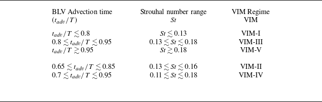
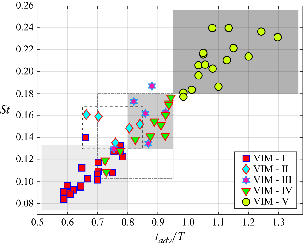
for these three VIM regimes are classified in table 2 and plotted in figure 7. Note that these boundaries are identified based on the presence of all/maximum cases in one particular type. There are very few minor exceptions (1 in 60 cases for classification based on
 $t_{\textit{ad}v}/T$
, and 2 in 60 cases for classification based on
 ${\textit{St}}$
) to these boundaries, namely, one case for VIM-III falls slightly below the time boundary
 $t_{\textit{ad}v}/T \lesssim 0.8$
, and one case each for VIM-I and VIM-III falls slightly above the upper
 ${\textit{St}}$
boundary (see figure 7). However, we have ensured that the interaction mechanisms for these three cases belong to the corresponding VIMs indicated in figure 7.
Quantitative basis, based on advection time of BLV over foil and Strouhal number, for categorisation of flow into five different VIMs.

The occurrence of the VIMs as a function of the BLV advection time (
 $t_{\textit{ad}v} / T$
) and the Strouhal number (
 ${\textit{St}}$
) for all the cases with flexible filaments. The rectangles highlight most/all cases pertaining to a particular VIM: rectangles with increasing intensity of grey colour correspond respectively to VIM-I, VIM-III, VIM-V; rectangles with broken and dash-dot lines correspond respectively to VIM-II and VIM-IV.

We observed that the vortex advection time, as well as the Strouhal number range for some cases, overlaps with the advection time scales and
 ${\textit{St}}$
range corresponding to VIM-I and VIM-III (see figure 7), as quantified in table 2. However, we found that the vortex interactions for these cases are very different from VIM-I and VIM-III (as discussed below), and hence, we grouped them into two distinct categories, namely, ‘VIM-II’ and ‘VIM-IV’.
Once the BLV enters over the flexible filament, it interacts with the TEV in three different ways, as discussed below.
-
(i) BLV merges with TEV near the TE and forms a vortex lump that rolls over the deforming filament. Such an interaction led to VIM-I.
-
(ii) BLV and TEV do not merge. Instead, they travel separately as isolated stretched vortices over the filament. The variations in post-shedding interactions of these vortices led to VIM-II, VIM-III and VIM-IV.
-
(iii) BLV merges with the TEV near the TE and forms a stretched vortex lump layer that slides over the deforming filament. Such an interaction led to VIM-V.
With this understanding on the basis for the classification of flow into different regimes, we will now discuss each VIM in detail by considering a representative case, focusing on the time evolution of the flow and the vortices. To illustrate each VIM, we choose seven snapshots of the representative case, as shown in figures 8 and 9.
Time-series snapshots to elucidate the evolution of the four VIMs. Columns correspond to VIMs – first from left: VIM-I (F2,
 ${\textit{St}} = 0.11$
); second: VIM-II (F2,
 ${\textit{St}} = 0.15$
); third: VIM-III (F2,
 ${\textit{St}} = 0.17$
); fourth: VIM-IV (F3,
 ${\textit{St}} = 0.16$
). Note that snapshots are selected at instants of important interaction activity instead of at regular intervals.

3.1. The case of VIM-I
We describe VIM-I using the left column of figure 8. At
 $t/T = 0.378$
, BLV-1 (under the red curve) is growing on the upper side of the foil, and TEV-2 (under the yellow curve) is present near the TE. The BLV-1 reaches near the TE (
 $t/T = 0.567$
) and rolls over TEV-2 (
 $t/T = 0.891$
). Then, BLV-1 and TEV-2 merge to form a single lump (1 + 2) at
 $t/T = 1.215$
. This lump reaches the filament tip (FT) at
 $t/T = 1.485$
and eventually is shed, followed by the shedding of SV array-6 (
 $t/T = 1.755$
). At
 $t/T = 2.025$
, array-6 of SVs is fully developed wherein the small vortices are nearly equispaced one behind the other, hence it is termed a ‘sequential array’ of SVs. Later, the lumped vortices (1 + 2) evolve into a PV with CW rotation. Ellipse-7 (
 $t/T = 2.025$
) encloses fluid that comes from the lower side of the filament, which would evolve into a CCW-PV (and another sequential SV array). Two PVs stay connected with array-6 of SVs on both of its ends. Subsequently, another CW-PV and SVs array would evolve from BLV-3 and TEV-4 (seen beyond
 $t/T = 1.485$
), similar to the evolution of BLV-1 and TEV-2.
In summary, in VIM-I, PVs are formed from the lump generated by the merger of BLVs and TEVs, and an array of SVs is generated sequentially from the trailing part of the lump.
3.2. The case of VIM-II
The second column of figure 8 illustrates VIM-II. The formation of BLV-1 and TEV-2 (until
 $t/T = 0.910$
) is similar to VIM-I; the difference is seen when they travel over the flexible filament. Instead of merging, BLV-1 and TEV-2 slide over the filament as two separate vortices (
 $t/T = 1.260$
). At
 $t/T = 1.540$
, TEV-2 is completely shed from the FT, while BLV-1 is partially shed and partially present on the filament. Then BLV-1 is completely detached from FT at
 $t/T = 1.785$
. Further (
 $t/T = 1.925$
), BLV-1 and TEV-2 merge to form a vortex lump (1 + 2). At the same time, array-6 of SVs grows from the trailing part of BLV-1. At
 $t/T = 2.240$
, array-6 of SVs is fully developed, and its front end is in contact with lumped vortices (1 + 2). Instead of forming a sequential pattern (as in VIM-I), the SVs in array-6 remain sparse with irregular spacing, hence we name it a ‘sparse array’. Later, lumped vortices (1 + 2) form CW-PV. The fluid coming from the lower side of the filament (ellipse-7,
 $t/T = 2.240$
) will evolve into a CCW-PV (that connects with the rear end of array-6) and an array of SVs below the CL. Following this event, another CW-PV and, subsequently, an array of SVs would evolve from BLV-3 and TEV-4 (present beyond
 $t/T = 1.540$
) in a similar way as BLV-1 and TEV-2 evolved.
Thus, in VIM-II, PVs are formed by merging BLVs and TEVs in the near-wake. The arrays of SVs are formed from the trailing part of the BLV.
3.3. The case of VIM-III
The third column of figure 8 shows images corresponding to VIM-III. Until
 $t/T = 1.287$
, BLV-1 and TEV-2 evolve similarly to VIM-II; a difference is seen when BLV-1 reaches the FT. At
 $t/T = 1.521$
, TEV-2 reaches the FT, and eventually gets shed as CW PV-2 (
 $t/T = 1.833$
) while BLV-1 is still stretched on the filament as a thin shear layer. The next instant (
 $t/T = 1.989$
) shows shedding of BLV-1 as array-1 of SVs whose front end is in contact with PV-2. At
 $t/T = 2.340$
, BLV-1 is fully developed as array-1 of SVs in which the small vortices are nearly equispaced (as in VIM-I); hence it is termed a ‘sequential array’. The fluid coming from the lower side of the filament (ellipse-7,
 $t/T = 2.340$
) will evolve into CCW-PV (that remains in contact with the rear end of array-1) and an array of SVs below the CL. Following this event, another CW-PV and, subsequently, an array of SVs would evolve from TEV-4 and BLV-3 (seen beyond
 $t/T = 1.521$
), similar to how TEV-2 and BLV-1 evolved. In summary, in VIM-III, TEVs and BLVs evolve respectively into PVs and a sequential array of SVs.
3.4. The case of VIM-IV
The last column of figure 8 corresponds to VIM-IV. The initial growth (
 $t/T = 0.666 {-} 1.073$
) of BLV-1 and TEV-2 is similar to VIMs–I, -II, -III; the main difference occurs during the shedding of the SV array. At
 $t/T = 1.480$
, TEV-2 has reached the FT ahead of BLV-1; simultaneously, BLV-3 and TEV-4 are sliding on the lower side of the filament. At the next instant (
 $t/T = 1.813$
), TEV-2 is already shed and is in the process of forming a CW-PV, and BLV-3 is being shed from the lower side. At
 $t/T = 2.442$
, CW PV-2 is fully developed, and BLV-3 is evolved into array-3 of SVs above the CL. Moreover, TEV-4 is in the process of forming a CCW-PV-4, while BLV-1 on the upper side of the filament is being shed from the FT. At
 $t/T = 2.886$
, TEV-4 is developed into CCW-PV-4, and BLV-1 has formed array-1 of SVs below the CL. Note that array-3 (array-1) of SVs originates from the lower (upper) side of the filament. We observed that the shape of the SV arrays (1, 3) is determined by the filament conditions near its tip, like the location, speed and direction of motion of the filament tip. The SVs are arranged sparsely and irregularly; hence, it is termed a ‘sparse array’.
In summary, in VIM-IV, CW-PV (CCW-PV) evolves from TEVs that come from the upper (lower) side of the filament. Moreover, the BLV on the upper (lower) side of the filament forms a sparse array of SVs below (above) the CL.
3.5. The case of VIM-V
At higher pitching frequencies, VIM-V (figure 9) is observed, that has the characteristics of VIM-I and VIM-IV. Similarly to VIM-I, BLV-1 and TEV-2 merge near the TE (
 $t/T = 1.760$
) and form a vortex lump (1 + 2) that continues to slide over the filament (
 $t/T = 2.288$
). A similar vortex lump (3 + 4) forms from BLV-3 and TEV-4 (
 $t/T = 2.288$
) that slides on the lower side of the filament (
 $t/T = 2.640$
). The lumped vortex (1 + 2) (shed from the FT at
 $t/T = 2.640$
) mainly develops into a CW-PV (
 $t/T = 2.816$
); however, its trailing part contributes to the formation of array-8 of SVs. Further, small vortices from the front end of the lumped vortex (3 + 4) also join the trailing part of array-8. At
 $t/T = 3.212$
, CW-PV and array-8 of SVs are fully developed. The major portion of the lumped vortex (3 + 4) that eventually evolves into a CCW-PV and an array of SVs (below the CL) is shown by ellipse-7 at
 $t/T = 3.388$
. Following this event, another CW-PV and, subsequently, an array of SVs, would evolve from the lumped vortices (5 + 6) formed from BLV-5 (
 $t/T = 2.640$
) and TEV-6 (
 $t/T = 3.388$
) in the same way as the vortex lump (1 + 2) evolved. We found that SVs in the array are spaced sequentially as well as sparse at different times, hence we call it a ‘mixed array’ of SVs.
Time-series images to illustrate VIM-V; F3,
 ${\textit{St}} = 0.20$
. Other details are the same as in figure 8.

In summary, in VIM-V, CW-PV (CCW-PV) evolves from the lump formed by BLV and TEV coming from the upper (lower) side of the filament. The leading and trailing portions of the vortex lump form small vortices that eventually evolve into an array of SVs on either side of the PVs.
3.6. Phenomenology of vortex interaction mechanisms
Schematic to illustrate the phenomenology of the five VIMs. Three different types of interactions between the BLV and TEV on the continuously deforming flexible filament are shown. It also depicts the interaction, shedding and evolution of the BLV and the TEV into PVs and SVs in the near-wake. The three representative time stamps (
 $t_{1}$
,
 $t_{2}$
,
 $t_{3}$
) marked in the figure correspond respectively to the events of BLV-TEV interaction over the filament, their shedding and the post-shedding interactions and evolution in the near-wake. The conventions are as follows: B – BLV, T – TEV, L – lump, P – PV, S – SVs, CL – centreline.

After providing a detailed account of each VIM, we now summarise the phenomenology of the VIMs. All five types of vortex interactions are schematically sketched in figure 10. As mentioned earlier, the advection time range of each VIM is different, and also, the BLV interacts with the TEV over the continuously deforming flexible filament in three different ways (see figure 10): they form a lump (VIM-I); both vortices travel as individual isolated stretched vortices (VIMs – II, III, IV); both vortices merge and travel as a stretched lump (VIM-V). The post-shedding interactions of either isolated BLV and TEV or the vortex lump of BLV and TEV in the near-wake and their eventual evolution into PVs and SVs occur in different ways, as discussed below (see figure 10 for details).
-
(i) For VIM-I: a major portion of the vortex lump (of BLV and TEV) sheds from FT as PV, while the trailing portion of the lump sheds as an array of SVs.
-
(ii) For VIM-II: two isolated stretched vortices (BLV and TEV) shed from the FT. But they merge in the near-wake to form a lump that evolves into a PV; the trailing portion of BLV forms an array of SVs.
-
(iii) For VIM-III: two isolated stretched vortices (BLV and TEV) shed from the FT. The TEV evolves into a PV, while the BLV forms an array of SVs.
-
(iv) For VIM-IV: two isolated stretched vortices (BLV and TEV) shed from the FT. The TEV coming from the upper (lower) side of the filament becomes a CW-PV (CCW-PV). The BLV coming from the upper (lower) side of the filament becomes SVs below (above) the CL.
-
(v) For VIM-V: a major portion of the stretched vortex lump (of BLV and TEV) from the upper (lower) side of the filament evolves into a CW-PV (CCW-PV). An array of SVs on both sides of the CL is formed from the contribution of vortex lumps coming from both sides of the filament.
Thus, the observations from the BLV advection time over the foil, different types of interactions of BLV and TEV over the deforming filament and finally, their interaction, shedding and evolution into PVs and SVs in the near-wake led us to categorise the flow into five different regimes of VIMs.
4. The
${\textit{St}}$
–
${\textit{EI}}$
phase maps


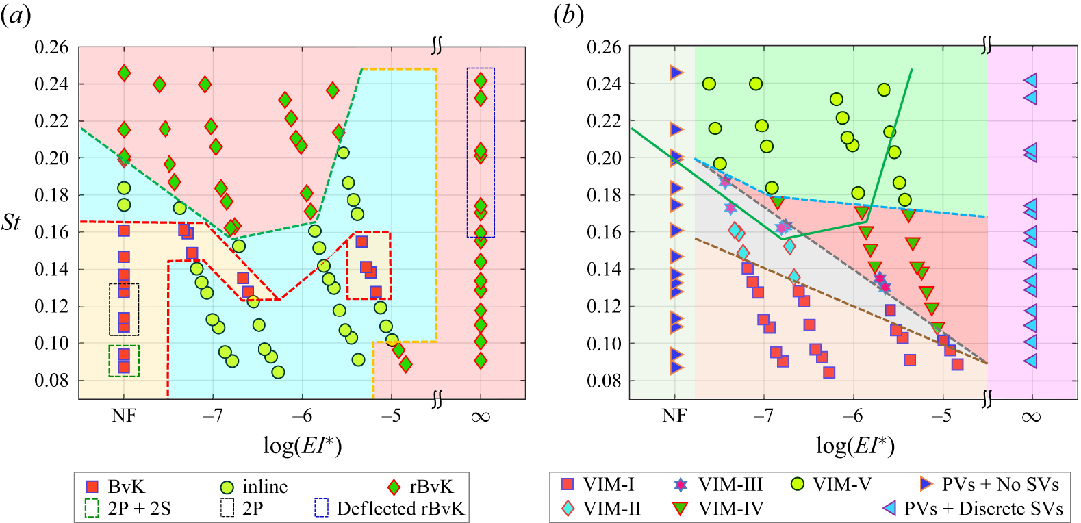
The filament flexibility and Strouhal number strongly influence the near-wake dynamics, resulting in a variety of vortex interactions and wake patterns (viz., BvK, inline, rBvK) which are summarised in the
 ${\textit{St}}$
–
 ${\textit{EI}}$
phase maps in figure 11 for all 90 cases.
4.1. Phase map of wake patterns
With an increase in the Strouhal number
 ${\textit{St}}$
, the pitching rigid foil follows the wake-transition route as BvK to inline to rBvK, indicative of drag to momentumless to thrust, respectively (Koochesfahani Reference Koochesfahani1989; Godoy-Diana et al. Reference Godoy-Diana, Aider and Wesfreid2008; Bohl & Koochesfahani Reference Bohl and Koochesfahani2009; Schnipper et al. Reference Schnipper, Andersen and Bohr2009; Andersen et al. Reference Andersen, Bohr, Schnipper and Walther2017); transition from inline to rBvK vortex street occurs beyond
 ${\textit{St}} \sim 0.18$
. Our rigid airfoil (NF) also follows the same transition route with the inline to rBvK cross-over at
 ${\textit{St}} \sim 0.20$
(figure 11
a). However, we find some interesting and counterintuitive transition trends when a flexible filament is attached to the rigid foil, and its flexural rigidity is varied over three orders of magnitude.
Figure 11(a) reveals that the flexible foil (with filaments F1, F2, F3, F4) does not follow the usual transition route. For the most flexible filament F1, the vortices align in the inline pattern for
 ${\textit{St}} \leqslant 0.14$
, beyond which the wake follows the usual transition trend (BvK to inline to rBvK). Filament F2 exhibits trends similar to F1, except that the inline pattern persists up to
 ${\textit{St}} \approx 0.12$
. Interestingly, for F3, the BvK pattern is not generated for any of the Strouhal numbers studied; instead, the inline vortex arrangement transitions directly to the rBvK pattern at
 ${\textit{St}} \approx 0.17$
. Increasing
 ${\textit{EI}}$
by two orders of magnitude shows even more complex transition trends. For the least flexible filament F4, the rBvK pattern is present for small
 ${\textit{St}}$
 $(\lesssim 0.1)$
. For
 $0.1 \lesssim {\textit{St}} \lesssim 0.12$
, an inline pattern is observed, which is followed by a BvK pattern for
 $0.12 \lesssim {\textit{St}} \lesssim 0.16$
. Beyond
 ${\textit{St}} \approx 0.16$
, an inline pattern is observed that transitions to rBvK street at
 ${\textit{St}} \approx 0.21$
.
The
 ${\textit{St}}$
–
 ${\textit{EI}}$
phase maps of (a) vortex street patterns in the near-wake and (b) VIMs, constructed based on all 90 cases. The data for the cases corresponding to the foil with NF and with a SF are included for completeness of the information, and also, to show how the wake flow and the transition patterns change when the rigid foil does not carry a flexible filament, when it carries a flexible filament and when its flexibility is gradually varied over several orders of magnitude, including the limiting case of SF. Coloured background patches segregate the cases corresponding to a particular wake pattern in (a) and VIM in (b). The broken green line in (a) marks the transition from inline to rBvK pattern; the same line is reproduced in (b) as a solid green line. In (b), broken brown, grey and cyan lines, respectively, mark the transitions from VIM-I to other VIMs, to VIM-IV from other VIMs and to VIM-V from other VIMs. At small
 ${\textit{St}}$
, the rigid foil (NF) sheds 2P and 2P + 2S patterns (see (a)); here, P – vortex pair, S – single vortex.

In the limiting case of a non-deformable SF (
 ${\textit{EI}} \rightarrow \infty$
), only the rBvK pattern is generated over the entire
 ${\textit{St}}$
range (
 $0.09 \lesssim {\textit{St}} \lesssim 0.24$
). Attaching a SF is just a rigid extension of foil with a total chord (1C + SF length). The
 ${\textit{St}}$
range based on tip-to-tip excursion of the SF tip is
 ${\textit{St}}_{FT} = 0.18{-}0.48$
, which is consistent with the
 ${\textit{St}}$
range of rigid foil for the rBvK pattern. Also, note in figure 11(a) that the foil with a SF generates a deflected/asymmetric rBvK vortex jet beyond
 ${\textit{St}}_{FT} \approx 0.32$
.
The phase map in figure 11(a) shows that attaching a flexible filament to a rigid foil slightly lowers the
 ${\textit{St}}$
for the rBvK cross-over, especially for more flexible filaments. The cross-over for filaments F1, F2, F3 occurs respectively, at around
 ${\textit{St}} \approx 0.18, 0.16, 0.17$
. Note that while attaching a SF to the foil generates a deflected rBvK jet at higher Strouhal numbers, the foil with flexible filament generates a symmetric rBvK vortex street (see figure 11
a). This change can be attributed to the stabilisation effects brought in by the presence of the foil flexibility, as reported earlier by Marais et al. (Reference Marais, Thiria, Wesfreid and Godoy-Diana2012), Shinde & Arakeri (Reference Shinde and Arakeri2014) and Zhu et al. (Reference Zhu, He and Zhang2014).
The phase map in figure 11(a) illustrates that introducing a flexible filament to the flapping foil and varying its flexibility revealed unusual transition patterns than those reported earlier for flapping rigid foils (e.g. Godoy-Diana et al. Reference Godoy-Diana, Aider and Wesfreid2008; Schnipper et al. Reference Schnipper, Andersen and Bohr2009). However, the underlying physical mechanisms behind such counterintuitive wake-transition trends are yet unknown and demand further detailed investigation. Although a recent study (Kim & Lee Reference Kim and Lee2019) reports that the role of LEVs, their interaction with the TEVs, and the ratio of LE and TE circulations are the crucial parameters in determining the wake transitions in flapping flexible foils, our pitching foil does not generate LEVs, and the transitions occur in their absence.
4.2. Phase map of VIMs
To investigate any possible connections of the vortex wake transitions to the VIMs identified in § 3, we construct the
 ${\textit{St}}$
–
 ${\textit{EI}}$
phase map for the VIMs observed for a flexible foil (see figure 11
b). While the foil without a filament and with SF largely sheds PVs, the addition of a flexible filament with different values of flexural rigidity (
 ${\textit{EI}}$
) reveals interesting vortex interaction variations with the Strouhal number (
 ${\textit{St}}$
), as shown in figure 11(b). Regardless of the
 ${\textit{EI}}$
value, VIM-I is observed for all four flexible filaments at small
 ${\textit{St}}$
; however, the
 ${\textit{St}}$
for the transition from VIM-I to other VIMs decreases with an increase in the
 ${\textit{EI}}$
value (broken brown line). At higher Strouhal numbers (
 ${\textit{St}} \gtrsim 0.18$
, excepting F1, for which it is slightly higher), VIM-V is observed for all flexible filaments (above the broken cyan line). For the intermediate Strouhal numbers, VIMs-II, -III and -IV are observed with increasing presence of VIM-IV for decreasing flexibility (the region between broken cyan and grey lines).
While only one type of vortex pattern is present in the case of a SF across all pitching frequencies studied (see figure 11 b), when the filament is made flexible, different types of vortex interactions and patterns emerge with changes in Strouhal number due to the generation of small SVs and their varied interactions with the PVs. Figure 11(b) reveals that when the filament is made more flexible, the variations in vortex interactions also increase.
Interestingly, the number of VIMs decreases with an increase in the flexural rigidity of the filament. The
 ${\textit{EI}}$
values of filaments F3 and F4 are, respectively, one and two orders higher than that of the filaments F1 and F2 (whose
 ${\textit{EI}}$
values are of the same order). Figure 11(b) shows that all the five VIMs (I–V) are present for F1 and F2; however, VIM-II and VIMs-II and -III are absent when the
 ${\textit{EI}}$
increases by one order (i.e. F2 to F3) and two orders (i.e. F2 to F4), respectively. In general, the
 ${\textit{EI}}$
value of the filament determines the type of VIMs that would be present in the flow. In other words, the particular VIMs can be associated with the order of magnitude of the filament’s flexural rigidity value.
The two phase maps in figure 11 generally show weak correspondence between the wake patterns and the VIMs, with the exception that VIM-V corresponds to the rBvK pattern for the flexible filaments. However, the rBvK pattern is seen in the presence of other VIMs as well, viz., VIM-III (F1), VIM-III and VIM-IV (F2), VIM-IV (F3), but at slightly lower Strouhal numbers.
5. Discussion and summary
Several parameters work together to influence the VIMs and the vortex wake patterns, namely, the pitching parameters (amplitude and frequency of pitching, pitch-point location), the flow parameters (free-stream velocity, fluid density, viscosity) and the geometrical and material properties of filament (flexural rigidity (
 ${\textit{EI}}$
), filament length, etc.). While the Strouhal number takes care of the amplitude and frequency of pitching and the free-stream flow velocity, to include the effects of the filament material and fluid properties, we define the non-dimensional flexural rigidity (
 $ {\textit{EI}}^ *$
) of the filament. We non-dimensionalise the flexural rigidity of the flexible filament (similar to Shinde & Arakeri Reference Shinde and Arakeri2014) as
 \begin{equation} {\textit{EI}}^ * = \frac {8 ({\textit{EI}})}{(1/2) \rho V_{\mathrm{TE}_{\textit{max}}}^2 l_f^3}, \end{equation}
where
 $\rho$
is the density of soap solution,
 $V_{\mathrm{TE}_{\textit{max}}}$
is the maximum velocity of the TE of the rigid foil and
 $l_{{\kern-1pt}f}$
is the chordwise length of the filament; for the 2-D film in this study, the fluid pressure force per unit span is considered. The details of non-dimensionalisation can be found in Shinde & Arakeri (Reference Shinde and Arakeri2014). The non-dimensional flexural rigidity (
 $ {\textit{EI}}^ *$
) considers the effects of the pitching parameters, fluid properties as well as filament properties, including its length. We construct the phase maps for the vortex street patterns and the VIMs using the non-dimensional flexural rigidity (
 $ {\textit{EI}}^ *$
). Figure 12 presents the semi-log plots of the
 ${\textit{St}}$
–
 ${\textit{EI}}^{*}$
phase maps.
The
 ${\textit{St}}{-} {\textit{EI}}^ *$
semi-log phase maps: (a) vortex street patterns in the near-wake; (b) VIMs. The
 $ {\textit{EI}}^ *$
values are plotted on a log scale. The data for the cases corresponding to the NF and SF foils are presented for completeness of information. Other details are the same as in figure 11.

The interactions between fluid and structure become highly coupled, intricate and complicated when the structure is flexible. One important and immediate effect of introducing flexibility to the flapping foil is the generation of several small SVs (as shown in figure 6). The evolution and interaction of SVs, along with their shedding pattern in relation to the big PVs, determine the vortex wake patterns. Thus, the vortex interactions and wake patterns are simultaneously governed by the flapping motion parameters and flow conditions (included in
 ${\textit{St}}$
), and the elasticity parameter and the geometrical features of the flexible structure (included in
 $ {\textit{EI}}^ *$
). To understand the effect of both
 ${\textit{St}}$
and
 $ {\textit{EI}}^ *$
on vortex interactions simultaneously, we form a new non-dimensional parameter by combining the Strouhal number and the non-dimensional flexural rigidity, and denote it by
 $\varUpsilon$
, as
 \begin{equation} \varUpsilon = {\textit{St}} \times {\textit{EI}}^ *. \end{equation}
This non-dimensional group is hereafter referred to as the ‘Yashavant number’ (
 $\varUpsilon$
).
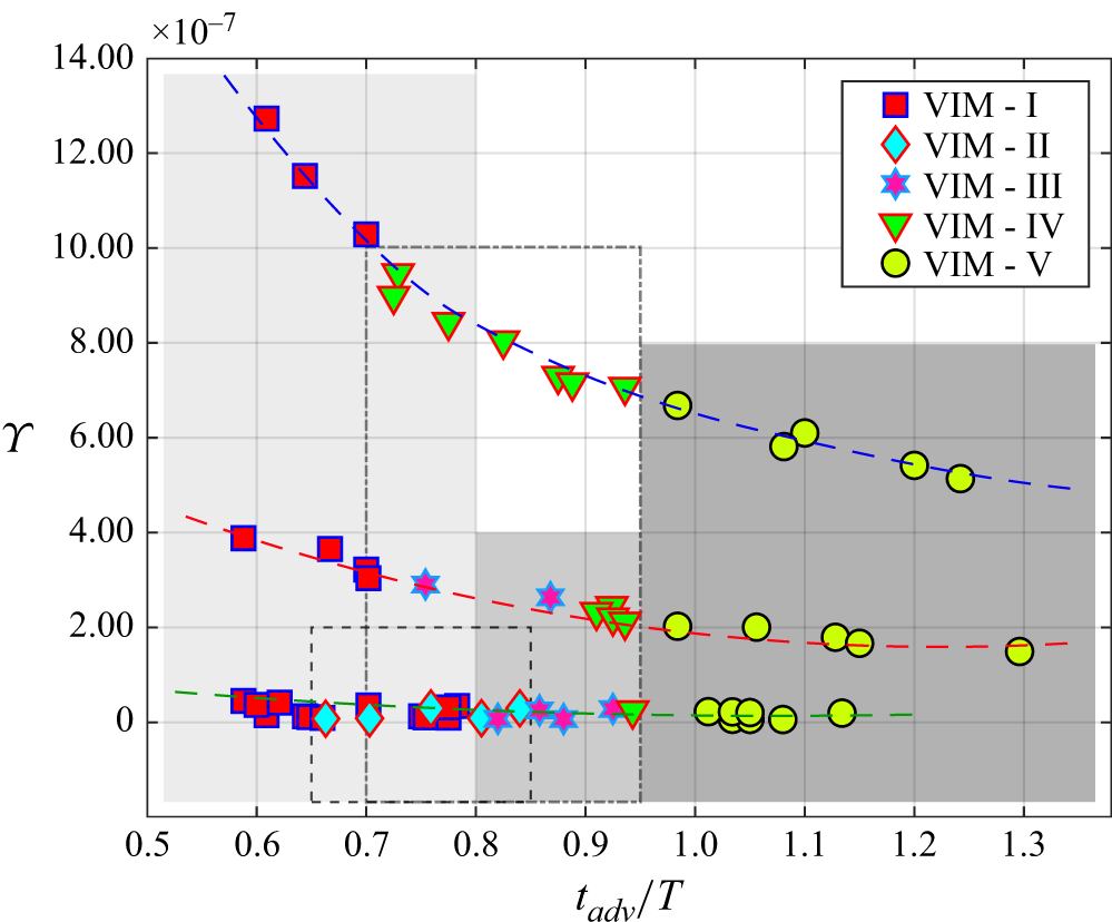
The dependence of the five VIMs on the BLV advection time
 $(t_{\textit{ad}v}/T)$
and the non-dimensional parameter that collectively includes several parameters in the fluid–structure interaction problem (see text), viz.,
 $\varUpsilon = {\textit{St}} \times {\textit{EI}}^ *$
. The rectangles, marked especially to indicate the BLV advection time boundaries of VIMs (see table 2), highlight most/all cases pertaining to a particular VIM: rectangles with increasing intensity of grey colour correspond respectively to VIM-I, VIM-III, VIM-V; rectangles with broken and dash-dot lines correspond respectively to VIM-II and VIM-IV. The broken curved lines are drawn to indicate the qualitative trends in the occurrence of VIMs on the
 $\varUpsilon$
–
 $(t_{\textit{ad}v}/T)$
plot.

Inserting the expressions for
 ${\textit{St}}$
and
 $ {\textit{EI}}^ *$
in (5.2), it emerges as,
 \begin{equation} \varUpsilon \sim \underbrace {\frac {1}{\rho U}}_{\text{Fluid and flow condition}} \boldsymbol{\cdot }\underbrace {\frac {\sin (\theta _{\textit{max}})}{ r \theta _{\textit{max}}^2}}_{\text{Flapping conditions}} \boldsymbol{\cdot }\underbrace {\frac {1}{l_f^3}}_{\text{Filament geometry}} \boldsymbol{\cdot }\frac {\textit{EI}}{f}, \end{equation}
where
 $r$
is the distance of the TE from the pitching point in terms of the fraction of the chord. It can be seen from (5.3) that
 $\varUpsilon$
encompasses the effects of several parameters involved in the complex fluid–structure interaction problem. In a simpler situation where the pitch-point location, pitch amplitude, length of flexible filament, fluid and flow velocity are kept constant (as in the present study),
 $\varUpsilon$
relates to two very important variables involved in the interaction of fluid with a flexible structure, as
 \begin{equation} \varUpsilon \sim \frac {\textit{EI}}{f}. \end{equation}
This parameter proves to be useful in identifying the VIMs and the wake patterns.
Figure 13 shows the variations in the vortex interactions with the newly formed parameter
 $\varUpsilon$
and the BLV advection time. We find that, in general, with the increase in
 $\varUpsilon$
, the number of VIMs decreases; a one order increase in
 $\varUpsilon$
decreases the number of VIMs by one. We find the following specific trends in the
 $\varUpsilon - (t_{\textit{ad}v}/T)$
plot (see figure 13).
-
(i) All five VIMs are present for small values of
$\varUpsilon \sim \mathcal{O} \, (10^{-8})$
(as marked by the bottom broken green curve in figure 13). -
(ii) Four VIMs are present for moderate values of
$\varUpsilon \sim \mathcal{O} \, (10^{-7})$
(broken red curve in the middle in figure 13). -
(iii) Three VIMs are present for relatively high values of
$\varUpsilon \sim \mathcal{O} \, (10^{-6})$
(broken blue curve at the top in figure 13). -
(iv) Only one type of vortex arrangement (i.e. rBvK, as shown in figure 6(f)), primarily with big vortices, is present in the extreme case with a SF for which
$\varUpsilon \rightarrow \infty$
. -
(v) VIM-I is predominantly present for small travel times of the BLV (
$t_{\textit{ad}v}/T \lesssim 0.8$
). -
(vi) Only VIM-V occurs for large BLV advection times (
$t_{\textit{ad}v}/T \gtrsim 0.95$
). -
(vii) VIM-III is present in the moderate time range (
$0.8 \lesssim t_{\textit{ad}v}/T \lesssim 0.95$
). -
(viii) VIM-II and VIM-IV are spread over both the small and moderate time spans; however, most cases corresponding to VIM-II are present in the small time range, while several cases of VIM-IV appear in the moderate time range.






Predicting what type of VIM is expected for a given combination of Strouhal number and flexural rigidity of flexible filament is indeed challenging, and it requires a more detailed systematic variation of filament
 $ {\textit{EI}}^ *$
. Such a study through experiments is heavily limited by the unavailability of filament materials of specific
 ${\textit{EI}}$
values; a numerical study would be convenient in this regard, provided the flow–structure solver is capable of handling the large nonlinear deformations of the filament. However, we find some general trends for the dependence of VIM occurrence on the BLV advection time and newly formed parameter
 $\varUpsilon$
, as discussed above and presented in figure 13.
The effect of foil shape and size on flow and transition in phase maps is investigated by Schnipper et al. (Reference Schnipper, Andersen and Bohr2009). They concluded that the wake structures and transition trends are insensitive to the foil dimensions as long as the foil is moderately thick and the
 $C/D$
ratio is greater than two. They also presumed that the qualitative structure of the phase diagram is insensitive to the value of the Reynolds number in the intermediate range between
 $10^2$
and
 $10^4$
since their 2-D flow is not subjected to the 3-D instabilities. The
 $C/D$
ratio of our foil is 6 (same as of the foil used by Schnipper et al. (Reference Schnipper, Andersen and Bohr2009)), our flow is two-dimensional and the Reynolds number,
 ${\textit{Re}} = U_\infty D / \nu = 330$
, is of the order of
 $10^2$
, that falls in the range prescribed by Schnipper et al. (Reference Schnipper, Andersen and Bohr2009). Moreover, for a purely plunging flexible teardrop airfoil (that is similar to our airfoil shape), Heathcote & Gursul (Reference Heathcote and Gursul2007) found that the effect of Reynolds number on the thrust coefficient, flow and efficiency is small; they explored the
 ${\textit{Re}}$
range of
 $10^3$
to
 $10^4$
. Furthermore, as mentioned earlier in § 2, our Reynolds number is comparable to the values used in previous studies on wake transition (for example, Godoy-Diana et al. Reference Godoy-Diana, Aider and Wesfreid2008; Schnipper et al. Reference Schnipper, Andersen and Bohr2009; Marais et al. Reference Marais, Thiria, Wesfreid and Godoy-Diana2012; Zhu et al. Reference Zhu, He and Zhang2014; Andersen et al. Reference Andersen, Bohr, Schnipper and Walther2017; Kim & Lee Reference Kim and Lee2019), and it falls in the intermediate range of the Reynolds number adopted by biological propulsion in nature (Wang Reference Wang2005). Therefore, as long as the foil shape is moderately thick, symmetric and aerodynamic, and the Reynolds number range is in the intermediate range of
 $10^2$
to
 $10^4$
, the leading foil type is not expected to significantly alter the flow patterns, phase maps and the VIM types.
The LEVs are not generated by the pitching foil in our experiments. The LE is blunt and rounded, the pitching point is very close to the LE (at
 $0.08 C$
from LE), and the pitching amplitude is small (
 $\theta _{\textit{max}} = \pm 6^{\circ }$
). Due to these reasons, the flow does not separate at the LE, and a clear LEV is not formed in any of the cases we studied. Numerical investigation on a heaving flexible foil by Kim & Lee (Reference Kim and Lee2019) showed that the important changes in the wake patterns and the thrust generation are largely keyed to the changes in the circulation around the LEVs, which are prominently generated in their case. However, the purely pitching flexible foil in our experiments does not generate LEVs. Therefore, the changes in the wake pattern, transition trends and vortex interactions (discussed in §§ 3 and 4) are in the absence of LEVs.
We summarise here the major findings from the present work. The wake transitions for rigid flapping foils are well studied, and the phase maps are well established (for example, Godoy-Diana et al. (Reference Godoy-Diana, Aider and Wesfreid2008), Schnipper et al. (Reference Schnipper, Andersen and Bohr2009), Andersen et al. (Reference Andersen, Bohr, Schnipper and Walther2017)). However, no such equivalent data, or phase maps are available for flexible foils, which are more closely related to the flapping appendages found in natural organisms, such as birds, fish and insects. Undertaken to bridge this gap, this study presents what is perhaps the first experimental investigation of the effect of flexibility on the transitions in the wake generated by flapping flexible foils. Our study provides, for the first time, the
 ${\textit{St}}$
–
 $ {\textit{EI}}^ *$
phase maps that account for the effects of flexural stiffness on VIMs and wake transitions. By spanning flexural rigidity over three orders of magnitude, we provide a phenomenology for VIMs. For flapping flexible foils, the wake-transition trends are not as usual (as reported for the flapping rigid foils). Instead, we find some counterintuitive trends that depend strongly on the filament’s flexibility or flexural rigidity. Several parameters simultaneously govern the interaction between the flexible structure and the fluid, thereby influencing the VIMs and wake patterns. We introduce a non-dimensional parameter (
 $\varUpsilon$
) to account for their combined effects. We clearly identify the dependence of the number of VIMs on the new parameter
 $\varUpsilon$
. While the type of VIMs is determined by BLV advection time, the number of VIMs is controlled by
 $\varUpsilon$
; one order increase in
 $\varUpsilon$
reduces the VIMs by one. The
 ${\textit{St}}$
–
 $ {\textit{EI}}^ *$
phase maps and the meticulous classification of vortex interactions into five newly identified mechanisms are expected to serve as a benchmark and to prove very useful for future studies of wake transition in flapping flexible foils, in addition to providing fundamental insight into the role of flexibility in wake transition.
We could not vary two other important parameters (filament length and pitch amplitude) in our experiments, which require a wider and longer film that is prone to sag and rupture. The chordwise length of the flexible foil and the flapping amplitude influence the wake flow (Alben et al. Reference Alben, Witt, Baker, Anderson and Lauder2012; Thulasi et al. Reference Thulasi, Menon, Jaiswara and Shinde2024). It would be interesting to explore how changes in filament length affect the wake transition, especially the interactions between the vortices (BLV and TEV) as they travel over highly deformed, flexible filaments with increased residence times. With the advent of numerical solvers for such fluid–structure interactions involving large nonlinear deformations, the effect of these parameters can be systematically explored to construct modified
 ${\textit{St}}$
–
 ${\textit{EI}}$
phase maps.
6. Conclusions
We experimentally investigate how flexibility alters vortex interactions and wake transitions and construct, perhaps for the first time, the
 ${\textit{St}}$
–
 ${\textit{EI}}$
phase maps for flapping flexible foils, which are closer to the natural flapping foils. Using a SFT, we studied the near-wake dynamics of a pitching foil with a flexible filament attached to its TE. The wide parameter space is explored by varying the filament flexibility over three orders of magnitude and a range of Strouhal numbers. Introducing flexibility to pitching foil results in the shedding of several small SVs along with big PVs, unlike only PVs for rigid foil. The generation and evolution of PVs and arrays of SVs depend on how the BLV and TEV interact when they travel over the continuously deforming flexible filament. With an extensive time-evolution analysis, we identified five VIMs and provided the phenomenology for the VIMs. The
 ${\textit{St}}$
–
 ${\textit{EI}}$
phase map of VIMs reveals interesting patterns. Regardless of flexural rigidity, the four filaments exhibit VIM-V at high (
 ${\textit{St}} \gtrsim 0.18$
) and VIM-I at small Strouhal numbers, albeit the transition
 ${\textit{St}}$
decreases with increasing
 ${\textit{EI}}$
. For the intermediate
 ${\textit{St}}$
range, VIM-IV is largely observed with the sparse presence of VIMs-II and -III. The number of VIMs decreases as the filament becomes more stiff; one order increase in
 ${\textit{EI}}$
reduces the number of VIMs by one, eventually leading to only one type of vortex arrangement for the limiting case of
 ${\textit{EI}} \rightarrow \infty$
.
The
 ${\textit{St}}$
–
 ${\textit{EI}}$
phase map of the vortex wake transitions revealed counterintuitive trends. With an increase in
 ${\textit{EI}}$
, the
 ${\textit{St}}$
for the transition to rBvK first decreases and then increases. Moreover, the flexible foil does not follow the usual transition route reported in the literature for rigid foil; instead, flexibility significantly alters the wake-transition trends. We observed the inline-to-BvK transition for more flexible filaments (F1, F2) and a direct transition from inline to rBvK, bypassing the BvK pattern for F3. For the least flexible filament (F4), the wake undergoes multiple transitions with increasing
 ${\textit{St}}$
. Comparison of the two
 ${\textit{St}}$
–
 ${\textit{EI}}$
phase maps indicates weak correspondence between wake patterns and VIMs, except that VIM-V generally corresponds to the rBvK pattern. While the previous studies show that the LEVs and circulation around them play a crucial role in the wake transitions, it is worth noting that the wake transitions in our experiments occur in the absence of the LEVs.
When the structure is flexible, the fluid–structure interactions turn highly intricate and coupled, and are governed by several parameters simultaneously. To include the parameters from flow, motion and the material properties of the fluid and structure, we normalise the flexural rigidity as
 $ {\textit{EI}}^ *$
, and devise a new non-dimensional parameter (‘Yashavant number’,
 $\varUpsilon$
) by combining it with
 ${\textit{St}}$
as
 $\varUpsilon = {\textit{St}} \times {\textit{EI}}^ *$
. We found that, while the type of VIM is largely determined by the BLV advection time, the number of VIMs is controlled by the parameter
 $\varUpsilon$
. We observed a clear trend in the occurrence of the VIMs with the new parameter: one order increase in
 $\varUpsilon$
decreases the number of VIMs by one. In the case of a SF for which
 $\varUpsilon \rightarrow \infty$
, only one type of vortex arrangement, primarily with big vortices, is present. The small, moderate and large BLV advection times, respectively, correspond to VIM-I, VIM-III and VIM-V. Although VIMs II and IV share the range of small and moderate BLV advection time, most cases corresponding to the former (latter) occur in the small (moderate) time range.
Although wake transitions for flapping rigid foils are rigorously studied and well understood, experimental investigations on the wake transition for flapping flexible foils with a systematic variation of flexibility are not available, to the best of our knowledge. Our study fills this gap and provides details on vortex interactions and wake transitions for flexible foils. Through the
 ${\textit{St}}$
–
 ${\textit{EI}}$
phase maps, we showed how flexibility alters vortex interactions and wake patterns. However, constructing more complete
 ${\textit{St}}$
–
 ${\textit{EI}}$
phase maps with systematic variations of filament length, flexural rigidity and pitch amplitude would serve as useful data for the use of flexible foils for bioinspired aquatic and aerial robots.
Supplementary movie
Supplementary movie is available at https://doi.org/10.1017/jfm.2026.11290.
Acknowledgements
We thank Akshay Menon, Chandan Pothal, and Keshav Birdi for useful discussions and inputs during the design and execution of the experiments. We are grateful to Professor Anurag Gupta for discussions on the filament stiffness calculations, and to Professor Anirban Guha and Professor Aditya Saurabh for several important discussions and invaluable inputs.
Declaration of interests
The authors report no conflicts of interests.