2 Governing equations

The two-dimensional, buoyancy-driven ascent of fluid through an environment of uniform density $\unicode[STIX]{x1D70C}_{0}$ from a line source at $z=0$ , issuing fluid of density $\unicode[STIX]{x1D70C}_{1}$ $(\unicode[STIX]{x1D70C}_{1}<\unicode[STIX]{x1D70C}_{0})$ is modelled in terms of the half-width of the mobile fluid, $b$ , the vertical velocity, $w$ , and the reduced gravity, $g^{\prime }=(\unicode[STIX]{x1D70C}_{0}-\unicode[STIX]{x1D70C}_{p})g/\unicode[STIX]{x1D70C}_{0}$ , where $\unicode[STIX]{x1D70C}_{p}$ is the density of the plume and $g$ is the magnitude of gravitational acceleration. The coordinate axes are aligned with $x$ horizontal and $z$ vertical (upwards), and the relative density of the plume fluid is sufficiently small $(\unicode[STIX]{x1D70C}_{0}-\unicode[STIX]{x1D70C}_{p})/\unicode[STIX]{x1D70C}_{0}\ll 1$ ) so that the motion is modelled under the Boussinesq approximation. On the assumption that the plume is relatively narrow so that the length scale of horizontal motion is much less than the length scale of vertical motion and consequentially, vertical pressure gradients are solely hydrostatic (Linden Reference Linden, Moffatt, Batchelor and Worster2000), and that viscous processes are negligible, integral expressions that represent conservation of mass, balance of vertical momentum and evolution of reduced gravity are given by

(2.1) $$\begin{eqnarray}\displaystyle & \displaystyle {\displaystyle \frac{\unicode[STIX]{x2202}b}{\unicode[STIX]{x2202}t}}+{\displaystyle \frac{\unicode[STIX]{x2202}}{\unicode[STIX]{x2202}z}}\int _{0}^{b}w\,\text{d}x=u_{e}, & \displaystyle\end{eqnarray}$$

(2.2) $$\begin{eqnarray}\displaystyle & \displaystyle {\displaystyle \frac{\unicode[STIX]{x2202}}{\unicode[STIX]{x2202}t}}\int _{0}^{b}w\,\text{d}x+{\displaystyle \frac{\unicode[STIX]{x2202}}{\unicode[STIX]{x2202}z}}\int _{0}^{b}w^{2}\,\text{d}x=\int _{0}^{b}g^{\prime }\,\text{d}x, & \displaystyle\end{eqnarray}$$

(2.3) $$\begin{eqnarray}\displaystyle & \displaystyle {\displaystyle \frac{\unicode[STIX]{x2202}}{\unicode[STIX]{x2202}t}}\int _{0}^{b}g^{\prime }\,\text{d}x+{\displaystyle \frac{\unicode[STIX]{x2202}}{\unicode[STIX]{x2202}z}}\int _{0}^{b}g^{\prime }w\,\text{d}x=0, & \displaystyle\end{eqnarray}$$

where $u_{e}$ is the entrainment velocity, representing the rate at which environmental fluid is engulfed into the line plume per unit area. (Axisymmetric versions of these equations were developed by Scase & Hewitt (Reference Scase and Hewitt2012) and Woodhouse et al. (Reference Woodhouse, Phillips and Hogg2016) and in appendix A, we derive these width-integrated expressions relevant for line plumes.) Crucially there is mixing between the environmental and buoyant fluids as the plume ascends due to the action of turbulent eddies and, following the seminal work of Morton et al. (Reference Morton, Taylor and Turner1956), we invoke the entrainment assumption and write $u_{e}=\unicode[STIX]{x1D6FC}w$ , where $\unicode[STIX]{x1D6FC}$ is a dimensionless constant. We comment that other studies have adopted different modelling strategies for representing the dynamics of turbulent plumes and in particular the mechanics of entrainment (Priestley & Ball Reference Priestley and Ball1955; Kaminski, Tait & Carazzo Reference Kaminski, Tait and Carazzo2005; Craske & van Reeuwijk Reference Craske and van Reeuwijk2016). These studies have formulated expressions for the transport, production and loss of mean kinetic energy, averaged over the horizontal cross-section of the plume and have then made a closure for the turbulent terms to form an integral model (see, for example, Craske & van Reeuwijk Reference Craske and van Reeuwijk2016). An important outcome of these approaches is that the entrainment coefficient emerges as a consequence of the modelling; it is not constant but is a function of the dependent variables and their gradients. These alternatives could be substituted within the modelling framework that follows, and the model of Craske (Reference Craske2017) extended to line plumes, is analysed in appendix C. To derive the width-averaged form, we introduce

(2.4a,b ) $$\begin{eqnarray}\int _{0}^{b}w\,\text{d}x=b\overline{w}\quad \text{and}\quad \int _{0}^{b}g^{\prime }\,\text{d}x=b\overline{g^{\prime }}.\end{eqnarray}$$

These expressions define the width-averaged vertical velocity and reduced gravity. We must also model the fluxes of momentum and buoyancy

(2.5a,b ) $$\begin{eqnarray}\int _{0}^{b}w^{2}\,\text{d}x=Sb\overline{w}^{2}\quad \text{and}\quad \int _{0}^{b}g^{\prime }w\,\text{d}x=S_{f}b\overline{w}\overline{g^{\prime }},\end{eqnarray}$$

where $S$ and $S_{f}$ are ‘shape factors’, which differ from unity when the dependent fields differ from ‘top-hat’ profiles (Craske & van Reeuwijk Reference Craske and van Reeuwijk2016; Woodhouse et al. Reference Woodhouse, Phillips and Hogg2016). In particular using (2.4), we note that

(2.6) $$\begin{eqnarray}(S-1)b\overline{w}^{2}=\int _{0}^{b}w^{2}\,\text{d}x-b\overline{w}^{2}=\int _{0}^{b}(w-\overline{w})^{2}\,\text{d}x\geqslant 0,\end{eqnarray}$$

and so $S\geqslant 1$ . Also we find that

(2.7) $$\begin{eqnarray}(S_{f}-1)b\overline{w}\overline{g^{\prime }}=\int _{0}^{b}(g^{\prime }-\overline{g^{\prime }})(w-\overline{w})\,\text{d}x,\end{eqnarray}$$

and therefore if the distributions of the reduced gravity and velocity fields are positively correlated then we anticipate $S_{f}\geqslant 1$ (Rouse et al. Reference Rouse, Yih and Humphreys1952; Anwar Reference Anwar1969); we focus on this regime in what follows (§§ 3 and 4), although we derive the results quite generally. (In appendix A we compute the shape factors on the assumption that the velocity and reduced gravity fields adopt Gaussian distributions about the centreline of the plume.) Provided the shape factors are constant, the governing system for $b$ , $\overline{w}$ and $\overline{g^{\prime }}$ is then given by

(2.8) $$\begin{eqnarray}\displaystyle & \displaystyle {\displaystyle \frac{\unicode[STIX]{x2202}b}{\unicode[STIX]{x2202}t}}+{\displaystyle \frac{\unicode[STIX]{x2202}}{\unicode[STIX]{x2202}z}}(b\overline{w})=\unicode[STIX]{x1D6FC}\overline{w}, & \displaystyle\end{eqnarray}$$

(2.9) $$\begin{eqnarray}\displaystyle & \displaystyle {\displaystyle \frac{\unicode[STIX]{x2202}}{\unicode[STIX]{x2202}t}}(b\overline{w})+S{\displaystyle \frac{\unicode[STIX]{x2202}}{\unicode[STIX]{x2202}z}}(b\overline{w}^{2})=b\overline{g^{\prime }}, & \displaystyle\end{eqnarray}$$

(2.10) $$\begin{eqnarray}\displaystyle & \displaystyle {\displaystyle \frac{\unicode[STIX]{x2202}}{\unicode[STIX]{x2202}t}}(b\overline{g^{\prime }})+S_{f}{\displaystyle \frac{\unicode[STIX]{x2202}}{\unicode[STIX]{x2202}z}}(b\overline{w}\overline{g^{\prime }})=0. & \displaystyle\end{eqnarray}$$

This system is the natural generalisation to planar geometry of the time-dependent model for axisymmetric plumes (Woodhouse et al. Reference Woodhouse, Phillips and Hogg2016). These governing equations (2.8)–(2.10) form a strictly hyperbolic set of equations when $S>1$ and $S_{f}\neq S\pm \sqrt{S^{2}-S}$ with characteristic directions given by

(2.11a,b ) $$\begin{eqnarray}{\displaystyle \frac{\text{d}z}{\text{d}t}}=S_{f}\overline{w}\quad \text{and}\quad {\displaystyle \frac{\text{d}z}{\text{d}t}}=(S\pm \sqrt{S^{2}-S})\overline{w}.\end{eqnarray}$$

When $S=1$ or $S_{f}=S\pm \sqrt{S^{2}-S}$ , the system is parabolic. These characteristic speeds are identical to the those for axisymmetric plumes up to a constant multiplicative factor (Woodhouse et al. Reference Woodhouse, Phillips and Hogg2016). When the system is hyperbolic, there may be solutions with discontinuities. Assuming the discontinuity is at $x=x_{s}(t)$ , the jump conditions across shocks are given by

(2.12a-c ) $$\begin{eqnarray}[b(\overline{w}-{\dot{x}}_{s})]_{x_{s}^{-}}^{x_{s}^{+}}=0,\quad [b\overline{w}(S\overline{w}-{\dot{x}}_{s})]_{x_{s}^{-}}^{x_{s}^{+}}=0\quad \text{and}\quad [b\overline{g^{\prime }}(S_{f}\overline{w}-{\dot{x}}_{s})]_{x_{s}^{-}}^{x_{s}^{+}}=0.\end{eqnarray}$$

These conditions conserve mass, momentum and buoyancy over the shock, respectively. In the special case $S_{f}=1$ there are two types of shocks satisfying these conditions. In one type the vertical velocity, $\overline{w}$ , and width of the line plume, $b$ , are discontinuous, but the reduced gravity, $\overline{g^{\prime }}$ is continuous. In the other, termed a contact discontinuity, the vertical velocity equals the shock speed $(\overline{w}={\dot{x}}_{s})$ and consequentially, the width must be continuous, but no condition is implied for the reduced gravity. As with the shallow water equations for fluid flows (e.g. Whitham Reference Whitham1974), we anticipate that terms neglected in the width-averaged plume equations (2.1)–(2.3), such as streamwise diffusion due to turbulent processes, will modify the structure of the solutions close to the discontinuities. However, away from these locations, and treated on length scales commensurate with the rest of the motion, the jump conditions (2.12) express conservation principles over the shock.

An important steady state of (2.8)–(2.10) corresponds to the motion generated by a sustained buoyancy flux at the line source. In this situation we enforce the ‘pure plume’ source conditions of a constant buoyancy flux per unit width, but vanishing mass and momentum fluxes at the origin ( $S_{f}b\overline{w}\overline{g^{\prime }}\rightarrow f_{1}$ , $b\overline{w}\rightarrow 0$ and $b\overline{w}^{2}\rightarrow 0$ as $z\rightarrow 0$ , where $2f_{1}$ denotes the constant buoyancy flux at the source). This steady state was derived by Lee & Emmons (Reference Lee and Emmons1961) for $S=S_{f}=1$ and is only slightly modified by the inclusion of shape factors, $S$ and $S_{f}$ . It is given by

(2.13a-c ) $$\begin{eqnarray}b=\unicode[STIX]{x1D6FC}z,\quad \overline{w}=\left({\displaystyle \frac{f_{1}}{\unicode[STIX]{x1D6FC}SS_{f}}}\right)^{1/3}\quad \text{and}\quad \overline{g^{\prime }}=\left({\displaystyle \frac{Sf_{1}^{2}}{\unicode[STIX]{x1D6FC}^{2}S_{f}^{2}}}\right)^{1/3}{\displaystyle \frac{1}{z}}.\end{eqnarray}$$

It is noteworthy that pure plume source conditions do not impose an independent length scale on the flow and consequently the dimensional dependences are determined solely in terms of the buoyancy flux per unit width, $f_{1}$ , and the distance from the source, $z$ (see Rouse et al. Reference Rouse, Yih and Humphreys1952). Thus the plume half-width grows linearly with distance from the source at a rate determined by the entrainment coefficient and is independent of the imposed buoyancy flux per unit width (see, for example, Morton et al. (Reference Morton, Taylor and Turner1956), Turner (Reference Turner1973)). The velocity of the steady line plume remains constant at the value determined by the source condition. This is in contrast to axisymmetric plumes from a point source for which the velocity decreases with distance from the source as $z^{-1/3}$ (Morton et al. Reference Morton, Taylor and Turner1956) and to line jets (where there is no density difference but a non-zero momentum flux per unit width at the source) for which the velocity decays as $z^{-1/2}$ (Bradbury Reference Bradbury1965). This illustrates the delicate balance in steady line plumes with the buoyancy forces that accelerate the fluid being in balance with the momentum drag due to the entrainment and acceleration of ambient fluid. In what follows we examine the time-dependent behaviour when the source condition is altered from an established steady pure plume.

3 Unsteady evolution: well-posedness and linear stability

We analyse the unsteady behaviour of line plumes and to this end, it is convenient to introduce dimensionless independent variables and to redefine the dependent variables such that the steady state (2.13) is scaled out. We introduce $\unicode[STIX]{x1D70F}=t/T$ , where $T$ is a relevant time scale of the motion, potentially set by time-dependent source conditions, and the dimensionless spatial variable is given by $\unicode[STIX]{x1D709}=z(\unicode[STIX]{x1D6FC}SS_{f}/f_{1})^{1/3}T^{-1}$ . The following dimensionless dependent variables are introduced:

(3.1a-c ) $$\begin{eqnarray}b=\unicode[STIX]{x1D6FC}z\hat{b}(\unicode[STIX]{x1D709},\unicode[STIX]{x1D70F}),\quad b\overline{w}=\left({\displaystyle \frac{\unicode[STIX]{x1D6FC}^{2}f_{1}}{SS_{f}}}\right)^{1/3}z\hat{q}(\unicode[STIX]{x1D709},\unicode[STIX]{x1D70F})\quad \text{and}\quad b\overline{g^{\prime }}=\left({\displaystyle \frac{\unicode[STIX]{x1D6FC}Sf_{1}^{2}}{S_{f}^{2}}}\right)^{1/3}{\hat{g}}(\unicode[STIX]{x1D709},\unicode[STIX]{x1D70F}).\end{eqnarray}$$

The governing equations can then be written in compact form by introducing $\boldsymbol{q}=(\hat{b},\hat{q},{\hat{g}})$ so that

(3.2) $$\begin{eqnarray}{\displaystyle \frac{\unicode[STIX]{x2202}\boldsymbol{q}}{\unicode[STIX]{x2202}\unicode[STIX]{x1D70F}}}+\left(\begin{array}{@{}ccc@{}}0 & 1 & 0\\ -S\hat{q}^{2}/\hat{b}^{2} & 2S\hat{q}/\hat{b} & 0\\ -S_{f}{\hat{g}}\hat{q}/\hat{b}^{2} & S_{f}{\hat{g}}/\hat{b} & S_{f}\hat{q}/\hat{b}\end{array}\right){\displaystyle \frac{\unicode[STIX]{x2202}\boldsymbol{q}}{\unicode[STIX]{x2202}\unicode[STIX]{x1D709}}}={\displaystyle \frac{1}{\unicode[STIX]{x1D709}}}\left(\begin{array}{@{}c@{}}\hat{q}(1-\hat{b})/\hat{b}\\ S({\hat{g}}-\hat{q}^{2}/\hat{b})\\ 0\end{array}\right).\end{eqnarray}$$

The steady state (2.13) corresponds to $\boldsymbol{q}=(1,1,1)$ and the buoyancy flux per unit width is $S_{f}b\overline{w}\overline{g^{\prime }}=f_{1}\hat{\jmath }$ , where the dimensionless flux is denoted by $\hat{\jmath }\equiv {\hat{g}}\hat{q}/\hat{b}$ .

We now consider the linear stability of the steady state in response to the introduction of small perturbations in the source conditions. Thus we write $\boldsymbol{q}=(1,1,1)+\unicode[STIX]{x1D716}\boldsymbol{q}_{1}$ , where $\unicode[STIX]{x1D716}$ is a small ordering parameter. We assume a harmonic perturbation at the source with angular frequency $\unicode[STIX]{x1D714}$ (so that $T=1/\unicode[STIX]{x1D714}$ ) and the linearised solution can be written as $\boldsymbol{q}_{1}=\exp (\unicode[STIX]{x1D719}(\unicode[STIX]{x1D709})+\text{i}\unicode[STIX]{x1D70F})\unicode[STIX]{x1D74D}(\unicode[STIX]{x1D709})$ . To determine linear stability, we must find the behaviour of the dependent variables in the far field (Woodhouse et al. Reference Woodhouse, Phillips and Hogg2016). The linearised governing equations are given by

(3.3) $$\begin{eqnarray}\unicode[STIX]{x1D63C}{\displaystyle \frac{\text{d}\unicode[STIX]{x1D74D}}{\text{d}\unicode[STIX]{x1D709}}}+\left(\unicode[STIX]{x1D63C}{\displaystyle \frac{\text{d}\unicode[STIX]{x1D719}}{\text{d}\unicode[STIX]{x1D709}}}+\unicode[STIX]{x1D63E}{\displaystyle \frac{1}{\unicode[STIX]{x1D709}}}+\text{i}\unicode[STIX]{x1D644}\right)\unicode[STIX]{x1D74D}=0,\end{eqnarray}$$

where $\unicode[STIX]{x1D644}$ is the identity matrix and the matrices $\unicode[STIX]{x1D63C}$ and $\unicode[STIX]{x1D63E}$ are given by

(3.4a,b ) $$\begin{eqnarray}\unicode[STIX]{x1D63C}=\left(\begin{array}{@{}ccc@{}}0 & 1 & 0\\ -S & 2S & 0\\ -S_{f} & S_{f} & S_{f}\end{array}\right)\quad \text{and}\quad \unicode[STIX]{x1D63E}=\left(\begin{array}{@{}ccc@{}}1 & 0 & 0\\ -S & 2S & -S\\ 0 & 0 & 0\end{array}\right).\end{eqnarray}$$

We seek expansions in the far field $(\unicode[STIX]{x1D709}\gg 1)$ of the form

(3.5a,b ) $$\begin{eqnarray}\unicode[STIX]{x1D719}=-\text{i}\unicode[STIX]{x1D706}\unicode[STIX]{x1D709}+\unicode[STIX]{x1D70E}\log \unicode[STIX]{x1D709}+{\displaystyle \frac{\unicode[STIX]{x1D6FE}}{\unicode[STIX]{x1D709}}}\ldots \quad \text{and}\quad \unicode[STIX]{x1D74D}=\unicode[STIX]{x1D74D}_{0}+{\displaystyle \frac{1}{\unicode[STIX]{x1D709}}}\unicode[STIX]{x1D74D}_{1}+{\displaystyle \frac{1}{\unicode[STIX]{x1D709}^{2}}}\unicode[STIX]{x1D74D}_{2}\ldots\end{eqnarray}$$

We substitute (3.5) into (3.3) and equate successive powers of $\unicode[STIX]{x1D709}^{-1}$ . At $O(1)$ we find that $\unicode[STIX]{x1D706}=\unicode[STIX]{x1D706}_{i}$ , where $1/\unicode[STIX]{x1D706}$ are eigenvalues of the matrix $\unicode[STIX]{x1D63C}$ and that $\unicode[STIX]{x1D74D}_{0}=\boldsymbol{e}_{Ri}$ are the associated eigenvectors. The eigenvalues, $\unicode[STIX]{x1D706}_{i}$ , and left and right eigenvectors, denoted $\boldsymbol{e}_{Li}$ and $\boldsymbol{e}_{Ri}$ , respectively $(i=1,2,3)$ , are given by

(3.6) $$\begin{eqnarray}\displaystyle & \displaystyle \unicode[STIX]{x1D706}_{1}=1/S_{f},\quad \boldsymbol{e}_{L1}^{T}=(S_{f}(S-S_{f}),S_{f}(S_{f}-1),(S_{f}-S)^{2}+S(1-S)), & \displaystyle\end{eqnarray}$$

(3.7) $$\begin{eqnarray}\displaystyle & \displaystyle \boldsymbol{e}_{R1}^{T}=(0,0,1), & \displaystyle\end{eqnarray}$$

(3.8) $$\begin{eqnarray}\displaystyle & \displaystyle \unicode[STIX]{x1D706}_{2,3}=1\pm {\displaystyle \frac{\sqrt{S^{2}-S}}{S}},\quad \boldsymbol{e}_{L2,3}^{T}=(-S\unicode[STIX]{x1D706}_{2,3},1,0), & \displaystyle\end{eqnarray}$$

(3.9) $$\begin{eqnarray}\displaystyle & \displaystyle \boldsymbol{e}_{R2,3}^{T}=(\unicode[STIX]{x1D706}_{2,3}(S_{f}\unicode[STIX]{x1D706}_{2,3}-1),S_{f}\unicode[STIX]{x1D706}_{2,3}-1,S_{f}\unicode[STIX]{x1D706}_{2,3}(\unicode[STIX]{x1D706}_{2,3}-1)). & \displaystyle\end{eqnarray}$$

We observe that

(3.10) $$\begin{eqnarray}\boldsymbol{e}_{L1}^{T}\unicode[STIX]{x1D63C}\,\boldsymbol{e}_{R1}=S_{f}((S_{f}-S)^{2}+S(1-S)),\end{eqnarray}$$

an expression that vanishes when $S_{f}=S\pm \sqrt{S^{2}-S}$ (i.e. when two of the characteristics coincide). Also we find that

(3.11) $$\begin{eqnarray}\boldsymbol{e}_{Li}^{T}\unicode[STIX]{x1D63C}\,\boldsymbol{e}_{Ri}=-2S(\unicode[STIX]{x1D706}_{i}-1)(S_{f}\unicode[STIX]{x1D706}_{i}-1)\quad \text{for }i=2,3.\end{eqnarray}$$

This expression vanishes when $S=1$ . It will be shown below when $S=1$ or when $S_{f}=S\pm \sqrt{S^{2}-S}$ that the subsequent analysis fails and that these cases require special attention; in these situations the system of governing equations (3.2) is no longer hyperbolic.

At $O(1/\unicode[STIX]{x1D709})$ , we apply the solvability condition and this yields

(3.12) $$\begin{eqnarray}\unicode[STIX]{x1D70E}_{i}\boldsymbol{e}_{Li}\unicode[STIX]{x1D63C}\,\boldsymbol{e}_{Ri}+\boldsymbol{e}_{Li}\unicode[STIX]{x1D63E}\,\boldsymbol{e}_{Ri}=0,\end{eqnarray}$$

for $i=1,2,3$ . Thus we deduce that provided $\boldsymbol{e}_{Li}\unicode[STIX]{x1D63C}\,\boldsymbol{e}_{Ri}$ is non-vanishing,

(3.13) $$\begin{eqnarray}\displaystyle & \displaystyle \unicode[STIX]{x1D70E}_{1} & \displaystyle ={\displaystyle \frac{S(S_{f}-1)}{(S-S_{f})^{2}+S(1-S)}}\end{eqnarray}$$

(3.14) $$\begin{eqnarray}\displaystyle & \displaystyle \text{and}\quad \unicode[STIX]{x1D70E}_{2,3} & \displaystyle =-2+{\displaystyle \frac{S(2S-1)\pm (S_{f}-2S)\sqrt{S^{2}-S}}{2S(S\mp \sqrt{S^{2}-S}-S_{f})}}.\end{eqnarray}$$

We note straightaway that this perturbative solution has failed when $S_{f}=S\pm \sqrt{S^{2}-S}$ since $\unicode[STIX]{x1D70E}_{1}$ and one of $\unicode[STIX]{x1D70E}_{2}$ and $\unicode[STIX]{x1D70E}_{3}$ are not defined at this value; this condition corresponds to the coincidence of two of the characteristic curves. However, when $S>1$ and $S_{f}\neq S\pm \sqrt{S^{2}-S}$ , the solutions grow or decay in the far field in proportion to $\unicode[STIX]{x1D709}^{\unicode[STIX]{x1D70E}_{i}}$ . These solutions due to a harmonic disturbance of the source are linearly stable when $\unicode[STIX]{x1D70E}_{i}\leqslant 0$ for $i=1,2,3$ and these inequalities are satisfied within regions of the $(S,S_{f})$ plane that we label as $R1$ and $R2$ , as depicted in figure 1. Recall that we anticipate that $S_{f}\geqslant 1$ and so we focus on region $R1$ , although the other region of stability, $R2$ , is included for completeness. In particular, region $R1$ is given by

(3.15) $$\begin{eqnarray}1\leqslant S_{f}\leqslant {\displaystyle \frac{2S(5S+1)+(10S+1)\sqrt{S^{2}-S}}{15S+1}}.\end{eqnarray}$$

Notably, when $S_{f}=1$ , the steady plume is linearly stable when

(3.16) $$\begin{eqnarray}S\geqslant {\displaystyle \frac{1}{2}}+{\displaystyle \frac{\sqrt{3}}{3}}.\end{eqnarray}$$

(cf. Woodhouse et al. (Reference Woodhouse, Phillips and Hogg2016) for axisymmetric plumes). Note further that if the shape factors for the momentum and buoyancy fluxes are equal $(S=S_{f})$ , then linear stability requires

(3.17) $$\begin{eqnarray}S\geqslant {\displaystyle \frac{1}{2}}+{\displaystyle \frac{3\sqrt{5}}{10}}.\end{eqnarray}$$

Figure 1.

The regions $R1$ and $R2$ within the plane of shape factors, $(S,S_{f})$ , for which the steady line plume solution (2.13) is stable to harmonic disturbances to the source (shaded region, bordered by dashed lines). Also plotted are the parameter values for which the governing system of equations are ill-posed (solid lines).

We observed above that particular values of the shape factors require special attention in order to determine their linear stability. First we examine the linear stability when $S=1$ and $S_{f}\neq 1$ . In this situation the eigenvalues are degenerate, $\unicode[STIX]{x1D706}_{2}=\unicode[STIX]{x1D706}_{3}=1$ , and so the system admits the following two eigenvalues and sets of vectors at leading order,

(3.18a-c ) $$\begin{eqnarray}\displaystyle \unicode[STIX]{x1D706}_{1}=1/S_{f},\quad \boldsymbol{e}_{L1}^{T}=(1,-1,-1+1/S_{f}),\quad \boldsymbol{e}_{R1}^{T}=(0,0,1), & & \displaystyle\end{eqnarray}$$

(3.19a-c ) $$\begin{eqnarray}\displaystyle \unicode[STIX]{x1D706}_{2}=1,\quad \boldsymbol{e}_{L2}^{T}=(1,-1,0),\quad \boldsymbol{e}_{R2}^{T}=(1,1,0). & & \displaystyle\end{eqnarray}$$

At $O(1/\unicode[STIX]{x1D709})$ , the solvability criterion (3.12) determines the growth rate $\unicode[STIX]{x1D70E}_{1}=1/(S_{f}-1)$ , but $\unicode[STIX]{x1D70E}_{2}$ is not determined because all the terms in (3.12) vanish. Thus we must proceed to higher order, for which we first find that $\unicode[STIX]{x1D74D}_{1}^{T}=\text{i}(\unicode[STIX]{x1D70E}_{2}+1)(1,0,-S_{f}/(1-S_{f}))$ . Then at $O(1/\unicode[STIX]{x1D709}^{2})$ , the solvability condition is given by

(3.20) $$\begin{eqnarray}\boldsymbol{e}_{L1}^{T}((\unicode[STIX]{x1D70E}_{2}-1)\unicode[STIX]{x1D63C}+\unicode[STIX]{x1D63E})\unicode[STIX]{x1D74D}_{1}=0,\end{eqnarray}$$

and this leads to $\unicode[STIX]{x1D70E}_{2}=-1$ and $\unicode[STIX]{x1D70E}_{2}=(2S_{f}-1)/(1-S_{f})$ . Thus when $S=1$ , linear stability requires that $S_{f}\leqslant 1/2$ .

When $S_{f}=S\pm \sqrt{S^{2}-S}$ , we need a different approach, because the eigenspace is degenerate (due to the coincidence of two of the characteristic curves) and the consequential singularities are not removable. In this case we construct the following series for $\unicode[STIX]{x1D719}(\unicode[STIX]{x1D709})$ and $\unicode[STIX]{x1D74D}(x)$ when $\unicode[STIX]{x1D709}\gg 1$ ,

(3.21a,b ) $$\begin{eqnarray}\unicode[STIX]{x1D719}=-\text{i}\unicode[STIX]{x1D706}\unicode[STIX]{x1D709}+\unicode[STIX]{x1D708}\unicode[STIX]{x1D709}^{1/2}+\unicode[STIX]{x1D70E}\log \unicode[STIX]{x1D709}+\cdots \quad \text{and}\quad \unicode[STIX]{x1D74D}=\unicode[STIX]{x1D74D}_{0}+{\displaystyle \frac{1}{\unicode[STIX]{x1D709}^{1/2}}}\unicode[STIX]{x1D74D}_{a}+{\displaystyle \frac{1}{\unicode[STIX]{x1D709}}}\unicode[STIX]{x1D74D}_{1}+\cdots \,.\end{eqnarray}$$

At leading order, we find two distinct eigenvalues, each of which have left and right eigenvectors. If we suppose that $\unicode[STIX]{x1D706}_{1}=\unicode[STIX]{x1D706}_{2}$ (see (3.7) and (3.9)) then the eigenvectors associated with this eigenvalue are

(3.22a,b ) $$\begin{eqnarray}\boldsymbol{e}_{L1}^{T}=(-S/S_{f},1,0)\quad \text{and}\quad \boldsymbol{e}_{R1}^{T}=(0,0,1),\end{eqnarray}$$

while the eigenvectors associated with eigenvalues $\unicode[STIX]{x1D706}_{3}$ are still given by (3.9). We substitute the revised series (3.21) into (3.3) and equate successive powers of $\unicode[STIX]{x1D709}^{-1/2}$ . At $O(\unicode[STIX]{x1D709}^{-1/2})$ we find that

(3.23) $$\begin{eqnarray}\unicode[STIX]{x1D74D}_{a}^{T}={\displaystyle \frac{\text{i}\unicode[STIX]{x1D708}S_{f}}{2(1-S_{f})}}(1,S_{f},0).\end{eqnarray}$$

The solvability criterion at $O(\unicode[STIX]{x1D709}^{-1})$ leads to

(3.24) $$\begin{eqnarray}\boldsymbol{e}_{L1}^{T}(\unicode[STIX]{x1D70E}\unicode[STIX]{x1D63C}+\unicode[STIX]{x1D63E})\boldsymbol{e}_{R1}+{\textstyle \frac{1}{2}}\unicode[STIX]{x1D708}\boldsymbol{e}_{L1}^{T}\unicode[STIX]{x1D63E}\unicode[STIX]{x1D74D}_{a}=0,\end{eqnarray}$$

and this implies that $\unicode[STIX]{x1D708}^{2}=2\text{i}/S_{f}$ . Furthermore we find that

(3.25) $$\begin{eqnarray}\unicode[STIX]{x1D74D}_{1}^{T}=-{\displaystyle \frac{\text{i}S_{f}}{2(S_{f}-1)^{2}}}(\unicode[STIX]{x1D70E}(S_{f}-1)-1,S_{f}(\unicode[STIX]{x1D70E}(S_{f}-1)+S_{f}-2),0).\end{eqnarray}$$

Finally we apply the solvability criterion at $O(\unicode[STIX]{x1D709}^{-3/2})$ to deduce

(3.26) $$\begin{eqnarray}\unicode[STIX]{x1D70E}=-{\displaystyle \frac{(4S_{f}^{2}-3S_{f}-2)}{8S_{f}(S_{f}-1)}}.\end{eqnarray}$$

There is one final important special case to consider, namely when both shape factors are set equal to unity, $S=S_{f}=1$ , a case that can only hold if the plume adopts piecewise constant velocity and density profiles (i.e. ‘top-hat’ profiles). In this situation there is only one eigenvalue, $\unicode[STIX]{x1D706}=1$ and a degenerate eigenspace. There are two independent left and right eigenvectors associated with this single eigenvalue, so we write

(3.27a,b ) $$\begin{eqnarray}\boldsymbol{e}_{R}^{T}=(1,1,a)\quad \text{and}\quad \boldsymbol{e}_{L}^{T}=(1+b,-1,-b),\end{eqnarray}$$

where $a$ and $b$ are real-valued. We substitute the series (3.21) into (3.3) and equate in successive powers of $O(\unicode[STIX]{x1D709}^{-1/2})$ . At each order of which we apply a solvability condition which must hold for all values of $a$ and $b$ , in addition to calculating the appropriate terms in the expansion of $\unicode[STIX]{x1D74D}$ . Thus we find that

(3.28a-c ) $$\begin{eqnarray}\unicode[STIX]{x1D74D}_{0}=(1,1,1),\quad \unicode[STIX]{x1D74D}_{a}=(\text{i}\unicode[STIX]{x1D708}/2,0,0)\quad \text{and}\quad \unicode[STIX]{x1D74D}_{1}=(\text{i}(\unicode[STIX]{x1D70E}+1),0,-\text{i}),\end{eqnarray}$$

while the solvability conditions imply

(3.29a,b ) $$\begin{eqnarray}\unicode[STIX]{x1D708}^{2}=4\text{i}\quad \text{and}\quad \unicode[STIX]{x1D70E}=-5/4.\end{eqnarray}$$

The implication of these last two derivations and results (3.26) and (3.29) for the special cases $S_{f}=S\pm \sqrt{S^{2}-S}$ and $S=S_{f}=1$ are that small disturbances grow exponentially in the far field: when $S=S_{f}=1$ the growth of the dependent variables is proportional to $\exp (\sqrt{2\unicode[STIX]{x1D709}})/\unicode[STIX]{x1D709}^{5/4}$ , while when $S_{f}=S\pm \sqrt{S^{2}-S}$ and $S\neq 1$ , the growth is proportional to $\exp (\sqrt{\unicode[STIX]{x1D709}/S_{f}})\unicode[STIX]{x1D709}^{\unicode[STIX]{x1D70E}}$ (where $\unicode[STIX]{x1D70E}$ is given by (3.26)). Reinserting the dimensional dependences for a harmonic disturbance of angular frequency $\unicode[STIX]{x1D714}$ , we find that the exponent of the exponential growth of the perturbation is proportional to $\unicode[STIX]{x1D714}^{1/2}$ and thus disturbances of high frequency grow with a larger exponent. Consequently, since a general disturbance, such as an instantaneous change of source buoyancy flux (see § 4), will feature all frequencies, the model is ill-posed because it will not be possible to resolve their dependence.

We may then summarise our findings from this investigation. If both shape factors are set to unity then the system of equations for the line plume are ill-posed and moreover ill-posedness remains if two of the characteristic curves coincide (so that $S_{f}=S\pm \sqrt{S^{2}-S}$ ). When the system is well-posed, there is the further constraint of linear stability, which here we define as bounded spatial evolution in the far field. This limits possible values of the shape factors $S$ and $S_{f}$ to lie within the regime depicted in figure 1 for which none of the growth rates are positive. In particular when $S_{f}=1$ , the models are linearly unstable when $1<S<S_{\ast }\equiv 1/2+\sqrt{3}/3$ and linearly stable when $S>S_{\ast }$ .

To confirm these predictions of linear stability we compute numerical solutions to the nonlinear governing equations (3.2) driven by a harmonic disturbance of small amplitude to the source condition. Our numerical method uses the central upwind scheme of Kurganov, Noelle & Petrova (Reference Kurganov, Noelle and Petrova2001) with a third-order total variation diminishing Runge–Kutta time stepping scheme and an adaptive time step that ensures that the Courant–Friedrichs–Lewy (CFL) number remains fixed at $1/2$ to maintain numerical stability (see Woodhouse et al. (Reference Woodhouse, Phillips and Hogg2016) for the application of this technique to axisymmetric plumes). We found that some numerical solutions required a relatively high spatial resolution to yield accurate results over our relatively large domains, but the run times are not excessively long. (For example, with a spatial resolution of $10^{-1}$ , a domain size of $10^{3}$ and runs over $10^{3}$ dimensionless time units, the numerical integration took 10 hours on a single processor desktop machine.)

We compare the predictions of linear stability to the numerical results by initiating the variables in the steady state, $\boldsymbol{q}(\unicode[STIX]{x1D709},0)=(1,1,1)$ , together with a small harmonic disturbance at the origin, $\boldsymbol{q}(0,\unicode[STIX]{x1D70F})=(1,1,1+\unicode[STIX]{x1D716}\text{e}^{\text{i}\unicode[STIX]{x1D70F}})$ . The magnitude of the perturbation $\unicode[STIX]{x1D716}$ , is chosen to be $10^{-2}$ or $10^{-3}$ so that the perturbations to the dependent fields remain sufficiently small throughout the entire domain and the dynamics are accurately captured by the linearised governing equations for which we have analytical predictions of the growth rate (see (3.14)). This perturbation is initiated at $\unicode[STIX]{x1D70F}=0$ and we compute over sufficient times to ensure that the higher harmonic transients associated with the initiation are advected out of the region of interest. We choose various values of the shape factors to illustrate the stability properties. 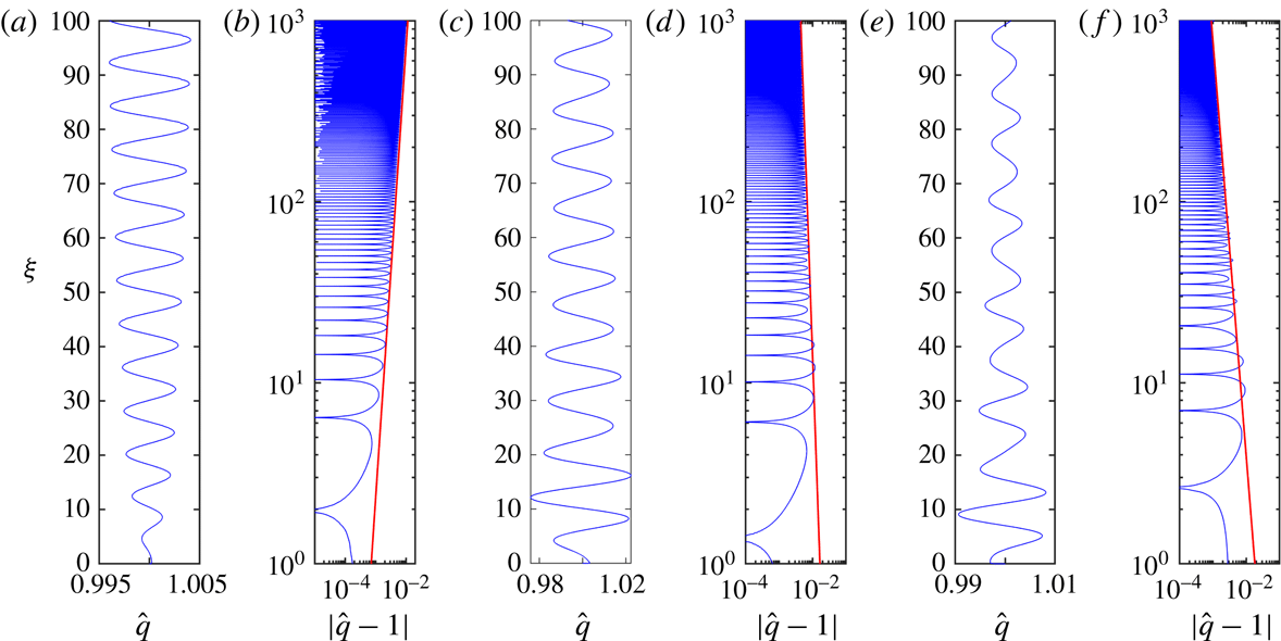First we examine $S_{f}=1$ and various values of $S$ (figure 2); we observe that the largest far-field growth rate, $\unicode[STIX]{x1D70E}_{3}$ in this case, accurately captures the numerical results for both an unstable value ( $S=1.05$ ) and for two stable values ( $S=1.1$ and $S=1.15$ ).

Figure 2.

The rescaled volume flux per unit width, $\hat{q}(\unicode[STIX]{x1D709},\unicode[STIX]{x1D70F})$ , as a function of dimensionless distance from source, $\unicode[STIX]{x1D709}$ , for the perturbed boundary condition $\boldsymbol{q}(0,\unicode[STIX]{x1D70F})=(1,1,1+\unicode[STIX]{x1D716}\text{e}^{\text{i}\unicode[STIX]{x1D70F}})$ and various values of the shape factor, $S$ , while $S_{f}=1$ in each case: (a,b) $\unicode[STIX]{x1D70F}=790$ and $S=1.05$ ; (c,d) $\unicode[STIX]{x1D70F}=699$ and $S=1.1$ ; (e,f) $\unicode[STIX]{x1D70F}=640$ and $S=1.15$ . Also plotted in (b), (d) and (f) are the theoretically predicted growth/decay rates.

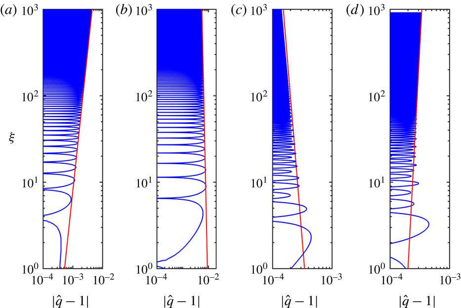
Next, in figure 3 we compare the far-field growth rates for the situation in which the two shape factors are equal $(S=S_{f})$ . In this figure we show results for unstable parameter values $(S=S_{f}=1.1)$ and for stable values $(S=S_{f}=1.2)$ , and again we observe that the theoretical analysis accurately captures the far-field growth rates. We also present brief numerical evidence to illustrate the stability boundary in region $R2$ (see figure 3). To this end we examine $(S,S_{f})=(1.4,0.5)$ for which the evolution is linearly stable and $(S,S_{f})=(1.5,0.5)$ for which the evolution is linearly unstable. Once more we find that the computationally determined growth/decay rates in the far field are accurately matched by the theoretical analysis.

Finally we examine the special case of $S=1$ . In this situation the governing system of partial differential equations is parabolic and exhibits just two independent sets of characteristic curves. In this case, it is simple to derive analytical expressions for the perturbed variables (see appendix B), which provide the complete linearised solutions and which confirm the far-field dependence; in particular it is demonstrated that the linearised solutions only decay in the far field if $S_{f}<1/2$ as determined above (see (3.20)). We also note that since the system is parabolic, we may no longer independently specify the values of all of the dependent variables at the source and that the numerical solution of the governing equations requires a different strategy since the problem is no longer hyperbolic. Henceforth we do not consider this special case further and restrict our attention to pairs of values of the shape factors drawn from the stable regions $R1$ and $R2$ as depicted in figure 1.

Figure 3.

The rescaled flux per unit width, $\hat{q}(\unicode[STIX]{x1D709},\unicode[STIX]{x1D70F})$ , as a function of dimensionless distance from source, $\unicode[STIX]{x1D709}$ , for the perturbed boundary condition $\boldsymbol{q}(0,\unicode[STIX]{x1D70F})=(1,1,1+\unicode[STIX]{x1D716}\text{e}^{\text{i}\unicode[STIX]{x1D70F}})$ and various values of the shape factors: (a) $\unicode[STIX]{x1D70F}=700$ and $S=S_{f}=1.1$ ; (b) $\unicode[STIX]{x1D70F}=592$ and $S=S_{f}=1.2$ ; (c) $\unicode[STIX]{x1D70F}=620$ , $S=1.4$ and $S_{f}=0.5$ ; (d) $\unicode[STIX]{x1D70F}=1450$ , $S=1.5$ and $S_{f}=0.5$ . Also plotted in (a–d) are the theoretically predicted growth/decay rates.

4 Plume dynamics in response to an abrupt change in buoyancy flux

We now consider the unsteady, nonlinear evolution that occurs when the source buoyancy flux per unit width changes abruptly from $f_{0}$ to $f_{1}$ at $\unicode[STIX]{x1D70F}=0$ . We find that the ratio of the old to the new buoyancy flux, ${\mathcal{F}}=f_{0}/f_{1}$ , is an important parameter in the dynamic response of the plume to the abrupt change in the source condition. Prior to the change in source conditions, the plume is in a steady state given by (2.13) with $f_{1}$ replaced by $f_{0}$ . After the new buoyancy flux has been imposed for sufficient time, the line plume will adjust to a new steady state given by (2.13). In this calculation we analyse the unsteady adjustment between these two steady states, which we show corresponds to a disturbance that is advected through the domain from the source. Furthermore we show that this adjustment occurs in a self-similar way and we construct the underlying similarity solutions, which we demonstrate depend on the ratio of the buoyancy fluxes, ${\mathcal{F}}$ , and the shape factors, $S$ and $S_{f}$ .

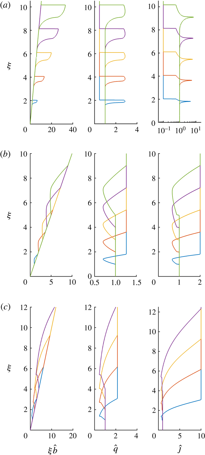
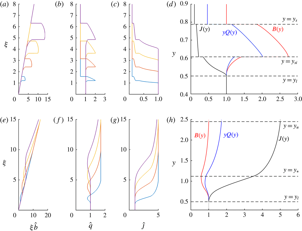
First we show the results from direct numerical integration of the governing equations (3.2) in a regime for which the model is well-posed and linearly stable (see § 3 and figure 2): we choose shape factors $(S,S_{f})=(1.1,1)$ and examine the response to different changes in the buoyancy flux per unit width. In all the cases plotted in figure 4, namely ${\mathcal{F}}=0.1$ , $2$ and $10$ , we see that the solution transitions from one steady state to another through the unsteady propagation of a growing region through the domain, and that the half-width of the line plume is independent of buoyancy flux when it has attained the steady state. We observe that when the source buoyancy flux is increased $({\mathcal{F}}<1)$ , the plume width increases throughout the transient region and that a shock emerges at the leading edge (figure 4 a). Conversely, for reductions in buoyancy flux $({\mathcal{F}}>1)$ that are relatively small, the plume narrows throughout the transient region, the leading and trailing edges connect continuously to the steady state (figure 4 b). Furthermore, when the reduction in the buoyancy flux becomes sufficiently large, there is an internal jump in the flow fields (compare the results for ${\mathcal{F}}=2$ and ${\mathcal{F}}=10$ , figures 4(b) and 4(c) respectively). We now analyse this motion in terms of similarity solutions and show how the adjustment from one steady state to another and the propagation of the transient region through the domain occur in a self-similar way.

Figure 4.

The rescaled width $\unicode[STIX]{x1D709}\hat{b}(\unicode[STIX]{x1D709})$ , volume flux $\hat{q}(\unicode[STIX]{x1D709})$ and buoyancy flux $\hat{\jmath }(\unicode[STIX]{x1D709})$ as functions of the dimensionless distance from source, $\unicode[STIX]{x1D709}$ , for various ratios of the source buoyancy flux, ${\mathcal{F}}$ imposed upon the system at $\unicode[STIX]{x1D70F}=0$ . (a) ${\mathcal{F}}=0.1$ and $\unicode[STIX]{x1D70F}=2,4,6,8,10$ ; (b) ${\mathcal{F}}=2$ and $\unicode[STIX]{x1D70F}=2,4,6,8,10$ ; (c) ${\mathcal{F}}=10$ and $\unicode[STIX]{x1D70F}=1,2,3,4$ . In all computations, $S=1.1$ and $S_{f}=1$ .

A line plume generated by an instantaneous change of buoyancy flux at the source has no externally imposed length or time scales. We therefore expect the adjustment to occur as a similarity solution in which vertical length scales are geared to the distance travelled by the buoyancy-induced motion. (In dimensional terms, $z\sim f_{1}^{1/3}t$ .) Thus we seek solution to (3.2) for $\boldsymbol{q}$ as functions of $y=\unicode[STIX]{x1D709}/\unicode[STIX]{x1D70F}$ . In fact it is convenient to seek solutions in terms of $(B(y),Q(y),G(y))=(\hat{b},\hat{q}/y,{\hat{g}}/y^{2})$ and under these definitions, we find that the similarity functions satisfy

(4.1) $$\begin{eqnarray}y\left(\begin{array}{@{}ccc@{}}-1 & 1 & 0\\ -SQ^{2}/B^{2} & 2SQ/B-1 & 0\\ -S_{f}GQ/B^{2} & S_{f}G/B & S_{f}Q/B-1\end{array}\right){\displaystyle \frac{\text{d}}{\text{d}y}}\left(\begin{array}{@{}c@{}}B\\ Q\\ G\end{array}\right)=\left(\begin{array}{@{}c@{}}-Q(2-1/B)\\ S(G-3Q^{2}/B)+Q\\ G(2-3S_{f}Q/B)\end{array}\right).\end{eqnarray}$$

We denote $\boldsymbol{Q}^{T}=(B,Q,G)$ and symbolically write this equation as $y\unicode[STIX]{x1D63F}\,\text{d}\boldsymbol{Q}/\text{d}y=\boldsymbol{b}$ for matrix $\unicode[STIX]{x1D63F}$ and vector $\boldsymbol{b}$ , which are functions of $\boldsymbol{Q}$ . The similarity equations and boundary conditions feature only the shape factors, $S$ and $S_{f}$ , and the buoyancy ratio  ${\mathcal{F}}$ .

We note that this system (4.1) admits a simple solution in which all of the dependent fields are constant $(B,Q,G)=(1/2,1/(3S_{f}),(2S-S_{f})/(3SS_{f}^{2}))$ . This solution corresponds to a ‘separable’ similarity solution, an analogous form of which has been identified for axisymmetric plumes (Scase et al. Reference Scase, Caulfield, Dalziel and Hunt2006; Craske & van Reeuwijk Reference Craske and van Reeuwijk2016) and line jets (Craske Reference Craske2017). However, as will be shown below, this simple solution does not satisfy the boundary conditions associated with an instantaneous change in buoyancy flux and so does not represent the ensuing dynamics. Instead, one must compute a spatially varying solution for $\boldsymbol{Q}$ in order to establish the similarity solution.

In the far field, $y\gg 1$ , the similarity solution adopts the steady state associated with the old buoyancy flux. Thus

(4.2) $$\begin{eqnarray}(B,Q,G)\rightarrow (1,{\mathcal{F}}^{1/3}/y,{\mathcal{F}}^{2/3}/y^{2})\quad \text{as }y\rightarrow \infty .\end{eqnarray}$$

Conversely, at the origin the solution adopts the steady state associated with the new buoyancy flux. Thus

(4.3) $$\begin{eqnarray}(B,Q,G)\rightarrow (1,1/y,1/y^{2})\quad \text{as }y\rightarrow 0.\end{eqnarray}$$

Both the behaviour in the far field (4.2) and near field (4.3) are, by construction, exact solutions to the similarity equations (4.1). More general solutions can only diverge from these exact forms at either discontinuities (‘shocks’) or at locations at which the matrix $\unicode[STIX]{x1D63F}$ is singular. In terms of the dimensionless variables, if a shock is located at $\unicode[STIX]{x1D709}_{s}=y_{s}\unicode[STIX]{x1D70F}$ , then denoting $W=Q/B$ , we find that the jump conditions (2.12) are given by

(4.4a-c ) $$\begin{eqnarray}[B(W-1)]_{y_{s}^{-}}^{y_{s}^{+}}=0,\quad [BW(SW-1)]_{y_{s}^{-}}^{y_{s}^{+}}=0\quad \text{and}\quad [G(S_{f}W-1)]_{y_{s}^{-}}^{y_{s}^{+}}=0.\end{eqnarray}$$

The matrix $\unicode[STIX]{x1D63F}$ is singular when $W=1/\unicode[STIX]{x1D707}$ , where $\unicode[STIX]{x1D707}=\unicode[STIX]{x1D707}_{1}\equiv S_{f}$ or $\unicode[STIX]{x1D707}=\unicode[STIX]{x1D707}_{\pm }\equiv S\pm \sqrt{S^{2}-S}$ . From the near-source solution (4.3), we thus deduce that the location closest to the source at which the solution can transition from its form with the new buoyancy flux is $y_{l}=\unicode[STIX]{x1D707}_{-}$ (provided $S-\sqrt{S^{2}-S}<S_{f}$ ), while the location furthest from the source beyond which the solution has adjusted completely to the old buoyancy flux is $y_{u}={\mathcal{F}}^{1/3}\unicode[STIX]{x1D707}_{+}$ (provided ${\mathcal{F}}^{1/3}(S+\sqrt{S^{2}-S})>S_{f}$ ). These correspond, respectively, to the slowest moving characteristic associated with the new buoyancy flux and the fastest characteristic associated with the old flux, originating from the source.

To integrate the similarity equations (4.1), we must numerically compute the solutions close to singular points of the governing system and it is valuable to use local series expansions for the dependent variables so that the numerical integration may avoid passing through these points. Thus we analyse the behaviour local to $y=y_{c}$ at which the dependent variables $\boldsymbol{Q}=\boldsymbol{Q}_{0}\equiv (B_{0},B_{0}/\hat{\unicode[STIX]{x1D707}},G_{0})$ , where $\hat{\unicode[STIX]{x1D707}}=\unicode[STIX]{x1D707}_{\pm }$ and $B_{0}$ and $G_{0}$ are as yet undetermined. (We note that the expansion for the singular points at which $\hat{\unicode[STIX]{x1D707}}=\unicode[STIX]{x1D707}_{1}$ takes a different form and must be treated separately.) We introduce the following expansion series for the dependent variables and functions of it,

(4.5) $$\begin{eqnarray}(\boldsymbol{Q},\unicode[STIX]{x1D63F},\boldsymbol{b})=(\boldsymbol{Q}_{0},\unicode[STIX]{x1D63F}_{0},\boldsymbol{b}_{0})+(y-y_{c})(\boldsymbol{Q}_{1},\unicode[STIX]{x1D63F}_{1},\boldsymbol{b}_{1})+(y-y_{c})^{\unicode[STIX]{x1D6FD}}(\boldsymbol{Q}_{\unicode[STIX]{x1D6FD}},\unicode[STIX]{x1D63F}_{\unicode[STIX]{x1D6FD}},\boldsymbol{b}_{\unicode[STIX]{x1D6FD}})+\cdots \,,\end{eqnarray}$$

where $\unicode[STIX]{x1D6FD}>0$ is not an integer. We substitute (4.5) into (4.1) and equate in successive powers of $(y-y_{c})$ . At $O(1)$ we find that

(4.6) $$\begin{eqnarray}y_{c}\unicode[STIX]{x1D63F}_{0}\boldsymbol{Q}_{1}=\boldsymbol{b}_{0}.\end{eqnarray}$$

The matrix $\unicode[STIX]{x1D63F}_{0}$ is singular and admits vectors $\boldsymbol{r}^{T}=(1,1,S_{f}G_{0}(1-\unicode[STIX]{x1D707}_{\pm })/(B_{0}(S_{f}-\unicode[STIX]{x1D707}_{\pm })))$ and $\boldsymbol{l}^{T}=(1,1-2\unicode[STIX]{x1D707}_{\pm },0)$ such that $\unicode[STIX]{x1D63F}_{0}\,\boldsymbol{r}=0$ and $\boldsymbol{l}^{T}\unicode[STIX]{x1D63F}_{0}=0$ . The solvability condition is $\boldsymbol{l}^{T}\boldsymbol{b}_{0}=0$ and this implies that

(4.7) $$\begin{eqnarray}G_{0}={\displaystyle \frac{1+(\unicode[STIX]{x1D707}_{\pm }-1)B_{0}}{\unicode[STIX]{x1D707}_{\pm }^{3}}}.\end{eqnarray}$$

The solution for $\boldsymbol{Q}_{1}$ is then given by

(4.8) $$\begin{eqnarray}\boldsymbol{Q}_{1}^{T}=\left(0,{\displaystyle \frac{1-2B_{0}}{y_{c}\unicode[STIX]{x1D707}_{\pm }}},-{\displaystyle \frac{(S_{f}-\unicode[STIX]{x1D707}_{\pm }(2-S_{f})B_{0}-(2\unicode[STIX]{x1D707}_{\pm }^{2}-(2+S_{f})\unicode[STIX]{x1D707}_{\pm }+S_{f})B_{0}^{2})}{y_{c}\unicode[STIX]{x1D707}_{\pm }^{3}B_{0}(S_{f}-\unicode[STIX]{x1D707}_{\pm })}}\right)+K\boldsymbol{r}^{T},\end{eqnarray}$$

where $K$ is an as yet undetermined constant. At $O(y-y_{c})$ we enforce a further solvability condition and this yields

(4.9) $$\begin{eqnarray}y_{c}\boldsymbol{l}^{T}\unicode[STIX]{x1D63F}_{1}\boldsymbol{Q}_{1}=\boldsymbol{l}_{1}^{T}\boldsymbol{b}_{1},\end{eqnarray}$$

which leads to two solutions for the constant $K$ , given by

(4.10a,b ) $$\begin{eqnarray}K_{1}={\displaystyle \frac{B_{0}-1}{y_{c}(\unicode[STIX]{x1D707}_{\pm }-1)}}\quad \text{and}\quad K_{2}={\displaystyle \frac{B_{0}(S_{f}\unicode[STIX]{x1D707}_{\pm }-2\unicode[STIX]{x1D707}_{\pm }^{2}+S_{f})+2\unicode[STIX]{x1D707}_{\pm }^{2}-(2S_{f}-1)\unicode[STIX]{x1D707}_{\pm }-2S_{f}}{2y_{c}\unicode[STIX]{x1D707}_{\pm }(\unicode[STIX]{x1D707}_{\pm }-1)(S_{f}-\unicode[STIX]{x1D707}_{\pm })}}.\end{eqnarray}$$

Next we consider the non-integer powers: at $O((y-y_{c})^{\unicode[STIX]{x1D6FD}-1})$ , we find $\unicode[STIX]{x1D6FD}y_{c}\unicode[STIX]{x1D63F}_{0}\boldsymbol{Q}_{\unicode[STIX]{x1D6FD}}=0$ , which has solution $\boldsymbol{Q}_{\unicode[STIX]{x1D6FD}}=K_{\unicode[STIX]{x1D6FD}}\boldsymbol{r}$ , where $K_{\unicode[STIX]{x1D6FD}}$ is a constant. At $O((y-y_{c})^{\unicode[STIX]{x1D6FD}})$ , we find that

(4.11) $$\begin{eqnarray}y_{c}\boldsymbol{l}^{T}(\unicode[STIX]{x1D63F}_{\unicode[STIX]{x1D6FD}}\boldsymbol{Q}_{1}+\unicode[STIX]{x1D6FD}\unicode[STIX]{x1D63F}_{1}\boldsymbol{Q}_{\unicode[STIX]{x1D6FD}})=\boldsymbol{l}^{T}\boldsymbol{b}_{\unicode[STIX]{x1D6FD}}.\end{eqnarray}$$

On substituting for each of the values of $K$ (see (4.8) and (4.10)), we find two values for $\unicode[STIX]{x1D6FD}$ (denoted $\unicode[STIX]{x1D6FD}_{1}$ and $\unicode[STIX]{x1D6FD}_{2}$ ), given by

(4.12) $$\begin{eqnarray}\unicode[STIX]{x1D6FD}_{1}={\displaystyle \frac{1}{\unicode[STIX]{x1D6FD}_{2}}}={\displaystyle \frac{B_{0}(3S_{f}\unicode[STIX]{x1D707}_{\pm }-2\unicode[STIX]{x1D707}_{\pm }^{2}-S_{f})+2S_{f}-\unicode[STIX]{x1D707}_{\pm }}{2B_{0}\unicode[STIX]{x1D707}_{\pm }(S_{f}-\unicode[STIX]{x1D707}_{\pm })}}.\end{eqnarray}$$

The constant $K_{\unicode[STIX]{x1D6FD}}$ remains undetermined and may be varied to generate different admissible solutions. The power series expansion in integer powers may be straightforwardly continued to higher powers if required, which leads to algebraically lengthy expressions that are conveniently handled using computer algebra.

Using the same methodology we may examine the behaviour close to a point $y=y_{c}$ at which $W(y_{c})=1/\unicode[STIX]{x1D707}_{1}$ (and $\unicode[STIX]{x1D707}_{1}=S_{f}$ ). We seek expansions for the dependent variables close to the location and find that

(4.13) $$\begin{eqnarray}\displaystyle \left(\begin{array}{@{}c@{}}B\\ Q\\ G\end{array}\right) & = & \displaystyle \left(\begin{array}{@{}c@{}}B_{0}\\ {\displaystyle \frac{B_{0}}{S_{f}}}\\ {\displaystyle \frac{B_{0}S_{f}(S-1)+(S_{f}-S)}{S_{f}^{2}S(S_{f}-1)}}\end{array}\right)+\,{\displaystyle \frac{(y-y_{c})}{y_{c}(S_{f}-1)}}\left(\begin{array}{@{}c@{}}B_{0}-1\\ -{\displaystyle \frac{(B_{0}(S_{f}-2)+1)}{S_{f}}}\\ -{\displaystyle \frac{2(B_{0}S_{f}(S-1)-S_{f}+S)}{(S_{f}^{2}S)}}\end{array}\right)\nonumber\\ \displaystyle & & \displaystyle +\,K_{\unicode[STIX]{x1D6FD}}(y-y_{c})^{\unicode[STIX]{x1D6FD}}\left(\begin{array}{@{}c@{}}0\\ 0\\ 1\end{array}\right)+\cdots \,,\qquad\end{eqnarray}$$

where the exponent is given by

(4.14) $$\begin{eqnarray}\unicode[STIX]{x1D6FD}={\displaystyle \frac{B_{0}S_{f}(S-1)+S_{f}-S}{B_{0}(S(S-1)-(S-S_{f})^{2})}}.\end{eqnarray}$$

It is notable that the leading-order term for $G$ in the expansion (4.13) becomes unbounded at $S_{f}=1$ because at that value of the shape factor, discontinuities in this field are advected with the local velocity field (i.e. a contact discontinuity, as noted in § 2).

We now construct the similarity solutions and demonstrate that they generate the nonlinear evolution computed directly from the governing partial differential equations. We illustrate three separate forms of solutions by first analysing $S_{f}=1$ , $S=1.1$ and various values of the changes in buoyancy flux, ${\mathcal{F}}$ . These reveal the generic forms of the solutions if $|S_{f}-S|<\sqrt{S^{2}-S}$ and the shape factors are drawn from region $R1$ (see figure 1). In appendix D we analyse the nonlinear motion when the shape factors are drawn from region $R2$ (figure 1). For these cases we find some additional features in the motion that arise due to an instantaneous change in buoyancy flux and we also construct the underlying similarity solutions (appendix D). In the results that follow (see figures 5, 7 and 10), we demonstrate that the solutions computed through the direct numerical integration of the governing equations (3.2) are indistinguishable from the similarity solutions that are computed using the methods described below.

4.1 Increase in buoyancy flux: ${\mathcal{F}}<1$

When there is an instantaneous increase in buoyancy flux at the source, the unsteady pulse that propagates through the domain features a shock at its leading edge $(y=y_{s})$ , at which the solution jumps from a faster moving state to the original buoyancy flux. The trailing edge corresponds to the slowest moving characteristic associated with the new flux $(y=y_{l})$ and in between there exists a location $(y=y_{\ast })$ at which the system is singular $(W=1)$ . Our method of constructing the solution numerically is as follows: we form a local series expansion for $|y-y_{l}|\ll 1$ , which entails the undetermined constant, $K_{\unicode[STIX]{x1D6FD}}$ , and given this value, we integrate the equations until $y=y_{\ast 1}$ at which $W=1/S_{f}=1$ and $B=B_{\ast 1}$ . We also choose a location for the shock at the leading edge, $y_{s}$ , and using the shock conditions (4.4), integrate backwards to $y=y_{\ast 2}$ at which $W=1$ and $B=B_{\ast 2}$ . We then adjust $K_{\unicode[STIX]{x1D6FD}}$ and $y_{s}$ until $y_{\ast 1}=y_{\ast 2}$ and $B_{\ast 1}=B_{\ast 2}$ . 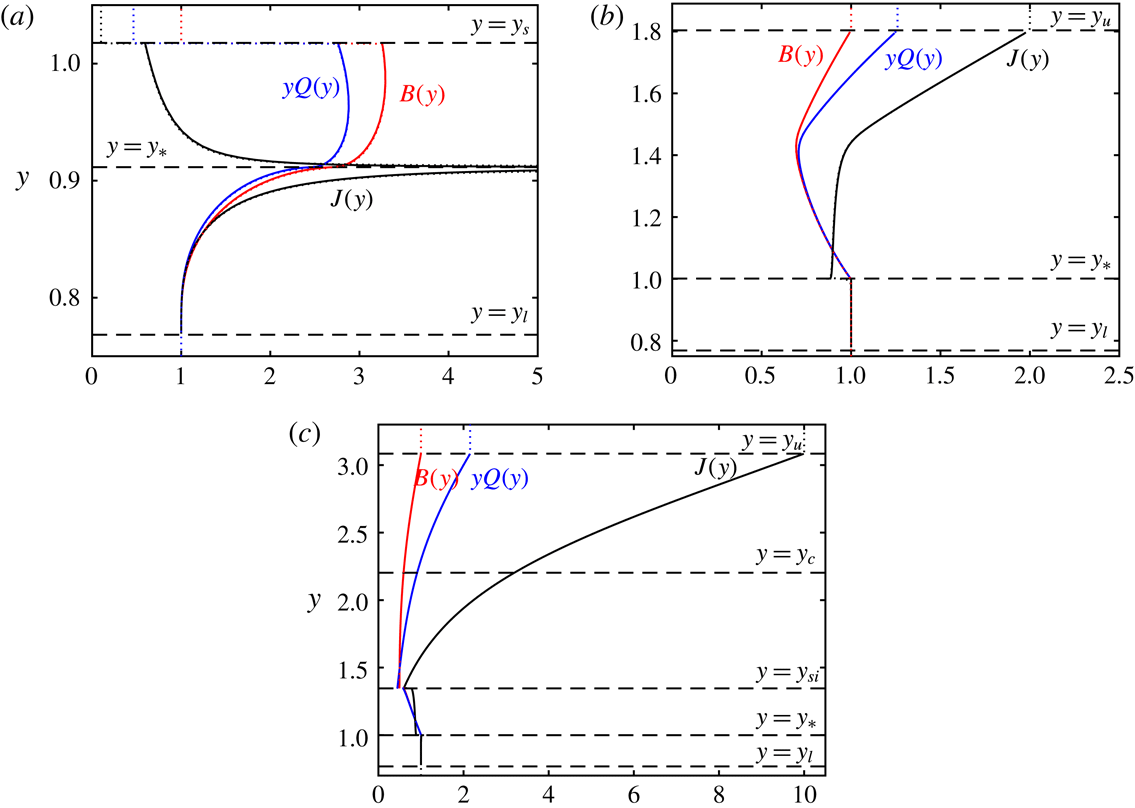The solution is plotted in figure 5(a) for ${\mathcal{F}}=0.1$ , in which we see that the plume broadens as it adjusts from the old steady state to the new and features the shock at its leading edge. We also find that as ${\mathcal{F}}$ is decreased, the width of the transition zone also decreases.

Figure 5.

(a–c) The similarity solutions for the width $B(y)$ , volume flux $yQ(y)$ and buoyancy flux $J(y)=y^{3}G(y)Q(y)/B(y)=\hat{\jmath }$ , for a line plume in response to an instantaneous change in source strength as functions of the similarity variable $y$ (solid lines) and their evaluation from direct numerical integration of (3.2) (dotted lines) for (a) ${\mathcal{F}}=10$ , (b) ${\mathcal{F}}=0.5$ , (c) ${\mathcal{F}}=0.1$ . In this case $S=1.1$ and $S_{f}=1$ . Also plotted are various important locations within the solution ( $y_{l}$ , $y_{\ast }$ , $y_{si}$ , $y_{c}$ , $y_{s}$ and $y_{u}$ ). Note that the similarity solution and numerical integration are virtually indistinguishable.

4.2 Weak decreases in buoyancy flux: $1<{\mathcal{F}}<{\mathcal{F}}_{m}(S)$ when $S<9/8$

When the buoyancy flux at the source instantaneously decreases $({\mathcal{F}}>1)$ , then the leading edge of the region within which the solution transitions from the old to the new flux is located at $y=y_{u}$ , corresponding to the fastest moving characteristic associated with the old flux originating from the source at $\unicode[STIX]{x1D70F}=0$ . Furthermore the solution is continuous at its leading edge. The transient zone then lies between $y_{l}$ and $y_{u}$ . We compute the similarity solution numerically by integrating separately from $y_{l}$ and $y_{u}$ towards locations at which $W=1$ . These numerical solutions are initiated by using the series expansions, each of which feature an undetermined constant multiplying the terms with non-integer powers. We adjust the constants until we find a solution for $W=1$ at $y=y_{\ast }$ and $B$ is continuous. We note from figure 5(b) for ${\mathcal{F}}=0.5$ that the plume narrows and accelerates as the buoyancy flux increases from its near-source value to its value in the far field.

Figure 6.

The regimes of similarity solutions in the $(S,{\mathcal{F}})$ plane for $S_{f}=1$ . Also plotted is the buoyancy flux ratio at source, at which internal shocks first appear, ${\mathcal{F}}_{m}$ , as a function of the shape factor $S$ (solid line). The value $S=1/2+\sqrt{3}/3$ is plotted (dashed line) and this corresponds to the threshold for linearly stable solutions, while solutions with internal shocks are not found for $S>9/8$ .

4.3 Strong decreases in buoyancy flux: ${\mathcal{F}}_{m}(S)<{\mathcal{F}}$ and $S<9/8$

When the decrease in buoyancy flux at the source is sufficiently large and $S<9/8$ , the similarity solution attains the singular value of $W=1/\unicode[STIX]{x1D707}_{+}$ both at the farmost extent of the transition zone $(y=y_{u})$ , but also at some interior location $(y=y_{c})$ at which the dependent variables are continuous. However, complete flow solutions can only be constructed consistently by introducing an internal shock at $y=y_{si}$ $(y_{si}<y_{c})$ , at which $W$ and $B$ are discontinuous. The solutions also pass through the critical point $y=y_{\ast }$ $(y_{\ast }<y_{si})$ at which $W=1$ and $B$ is continuous before connecting with the solutions emanating from $y_{l}$ .

The solution is most easily constructed numerically as follows. Values of four variables are assumed, namely the location $y_{c}$ and $B(y_{c})=B_{0}$ at which $W(y_{c})=1/\unicode[STIX]{x1D707}_{+}$ , the location of the internal shock, $y_{si}$ , and the value of the constant, $K_{\unicode[STIX]{x1D6FD}}$ , multiplying the non-integer powers in the series expansion close to $y_{l}$ . Given these choices, we integrate from $y=y_{c}$ to $y=y_{u}$ , using series expansions to initiate the numerical integration and evaluate $N_{1}=B(y_{u})-1$ and $N_{2}=G(y_{u})-{\mathcal{F}}^{2/3}/y_{u}^{2}$ . We also integrate from $y=y_{c}$ to $y=y_{si}$ at which point we apply the shock conditions to evaluate the jump in values of $B$ and $W$ . We then integrate to $y=y_{\ast 2}$ at which $W(y_{\ast 2})=1$ and $B(y_{\ast 2})=B_{\ast 2}$ . We also integrate from $y=y_{l}$ to $y=y_{\ast 1}$ at which $W(y_{\ast 1})=1$ and $B(y_{\ast 1})=B_{\ast 2}$ , and then evaluate $N_{3}=y_{\ast 1}-y_{\ast 2}$ and $N_{4}=B_{\ast 1}-B_{\ast 2}$ . We iteratively adjust the values of $y_{c}$ , $B_{0}$ , $y_{si}$ and $K_{\unicode[STIX]{x1D6FD}}$ until $N_{1}=N_{2}=N_{3}=N_{4}=0$ . A typical solution in plotted in figure 5(c), in which the narrowing of the plume is evident in addition to the internal shock across which the dependent variables change discontinuously.

The ratio of the buoyancy fluxes at which an internal jump first appears depends upon the shape factor, $S$ and is denoted ${\mathcal{F}}_{m}(S)$ . When $1\leqslant {\mathcal{F}}<{\mathcal{F}}_{m}$ , solutions without an internal jump are found. Instead, when ${\mathcal{F}}={\mathcal{F}}_{m}$ the solution exhibits a discontinuous gradient at the internal singular point $y=y_{c}$ and the series expansion switches from featuring $K_{2}$ to $K_{1}$ (4.10). In this way, we can evaluate ${\mathcal{F}}_{m}$ and it is plotted in figure 6. The limiting case occurs when the gradients of $W$ and $B$ vanish at $y=y_{c}$ , which from (4.8) and (4.10) occurs at $B_{0}=1/2$ and $\unicode[STIX]{x1D707}_{+}=3/2$ (and consequentially $S=9/8$ ). Thus we find that only continuous solutions arise for ${\mathcal{F}}>1$ when $S>9/8$ . The regimes of solutions are depicted in figure 6.

Figure 7.

(a–c) The rescaled width $\unicode[STIX]{x1D709}\hat{b}(\unicode[STIX]{x1D709})$ , volume flux $\hat{q}(\unicode[STIX]{x1D709})$ and buoyancy flux $\hat{\jmath }(\unicode[STIX]{x1D709})$ as functions of the dimensionless distance from source, $\unicode[STIX]{x1D709}$ , for an instantaneous increase in the buoyancy flux per unit width at the origin $({\mathcal{F}}=0.1)$ at dimensionless times $\unicode[STIX]{x1D70F}=2,4,6$ and 8. (d) The similarity solution for $B(y)$ , $Q(y)$ and $J(y)$ as functions of the similarity variable, $y$ (solid lines), and the results from the direct numerical integration of the governing equations (3.2) (dotted lines). Note that the two solutions are virtually indistinguishable. Also shown are three important locations $(y_{l},y_{si},y_{s})$ in the construction of the similarity solution. In these computations, $S=1.2$ and $S_{f}=1.2$ .

5 Summary and conclusions

In this study we have developed a well-posed, integral model for the unsteady motion of line plumes and have demonstrated the need to account for the variation of the vertical velocity and the reduced gravity across the plume, rather than assuming they adopt ‘top-hat’ distributions. This introduces shape factors, $S$ and $S_{f}$ , that are related to the variance of the distribution of vertical velocity and the covariance of the distributions of vertical velocity and reduced gravity, respectively. Both shape factors are equal to unity if these fields adopt ‘top-hat’ profiles and crucially this leads to an ill-posed system of time-dependent equations. Such a system cannot be used for computing temporally varying flows. This result extends to line plumes what has been established for axisymmetric plumes (Scase & Hewitt Reference Scase and Hewitt2012; Craske & van Reeuwijk Reference Craske and van Reeuwijk2016; Woodhouse et al. Reference Woodhouse, Phillips and Hogg2016). We have also demonstrated that ill-posedness can arise when $S_{f}=S\pm \sqrt{S^{2}-S}$ . With the additional constraint of linear stability, which requires perturbations to decay in the far field, we showed that this restricts the admissible values of the shape factors to certain regions of the $(S,S_{f})$ -plane (figure 1). We calculated the asymptotic growth/decay rates in the far field in response to a sustained harmonic disturbance to ‘pure’ plume source conditions and confirmed these predictions by direct numerical integration of the governing system of three partial differential equations that express mass and buoyancy conservation and the balance of vertical momentum. It is interesting to note that these distributions of velocity and reduced gravity, captured here through shape factors, play a significant role in unsteady integral models, but not in the steady states which are essentially determined through dimensional reasoning. We also comment that since these deductions are based upon the far-field behaviour, we anticipate that the results will carry over to the stability of steady states for ‘forced’ and ‘lazy’ line plumes in which the source conditions are not in ‘pure’ plume balance (see van den Bremer & Hunt (Reference van den Bremer and Hunt2014)). Solutions with such source conditions adjust to solutions generated by ‘pure’ plume conditions sufficiently far from source and thus the same far-field deductions about linear stability follow (see § 3).

When there is an instantaneous change in the buoyancy flux per unit width at the source, the line plume adjusts from one steady state to another though a transient ‘pulse’ that advects through the domain. This nonlinear adjustment occurs in a self-similar way. We determined the similarity solutions that underlie this motion; these are functions of the similarity variable for which the vertical length, $z$ , is geared linearly to time, $t$ . Essentially the self-similarity arises because there are no externally imposed length or time scales in the flow, other than the buoyancy flux per unit width at the source. We showed how the nonlinear adjustment is a function of the ratio of the old to new buoyancy fluxes and the shape factors. For instantaneous increases in the buoyancy flux per unit width, we found that the transient response is led by a shock over which the dependent variables are discontinuous. The plume broadens and slows toward the leading edge as the dynamics adjust to meet the previously established steady state. Conversely, for an instantaneous decrease in buoyancy flux per unit width, we found that the plume narrows and accelerates. The similarity solutions feature internal shocks and critical points at which the gradients of dependent variables change discontinuously. We showed that the similarity forms could be computed by integrating the three coupled ordinary differential equations that arise from the governing system and described the numerical strategies required for applying the appropriate boundary conditions for various values of the shape factors and ratio of old to new buoyancy fluxes per unit width at the source.

Models of unsteady line plumes are closely related to their axisymmetric counterparts, although the geometrical change leads to several differences in their behaviour. The integral models for line and axisymmetric plumes both feature two shape factors (cf. Woodhouse et al. Reference Woodhouse, Phillips and Hogg2016) and the magnitude of these factors leads to situations in which steady solutions may be linearly stable or unstable, as well as the governing equations exhibiting ill-posedness (Scase & Hewitt Reference Scase and Hewitt2012). In this study we have analysed variations of both shape factors, adding to the more restrictive study by Woodhouse et al. (Reference Woodhouse, Phillips and Hogg2016) of axisymmetric plumes, which analysed just the variation of $S$ . Furthermore the thresholds of stability differ in each of the two configurations. For instantaneous changes of the buoyancy flux per unit width at the source, we have shown that the line plumes adjust to the new steady state via similarity solutions. Analogous behaviour was found for axisymmetric plumes (Woodhouse et al. Reference Woodhouse, Phillips and Hogg2016), but for line plumes the gearing between temporal and spatial scales, which underpins the self-similarity form, differs from their axisymmetric counterparts.

Measurements of plumes are often used to infer geophysical characteristics of the source. For example, observations of line plumes generated by volcanic activity in submarine (such as lava extrusion during seafloor spreading events which produce hydrothermal plumes in the ocean, e.g. Baker et al. (Reference Baker, Massoth, Feely, Embley, Thomson and Burd1995)) and subareal (such as fissure eruptions that produce line plumes of volcanic gases and ash, e.g. Glaze, Baloga & Wimert (Reference Glaze, Baloga and Wimert2011)) settings are used to determine the fluxes of mass and heat from the intruding magmatic source. Arguably the simplest observation to make is to image the visible edge of the plume. Our analysis demonstrates that the development of transient pulses that propagate through the plume preserve information on the unsteady source condition. Thus image sequences, appropriately averaged and analysed, could be utilised to indicate temporal variations in the source conditions and provide greater insight into the geological processes that produce plumes in the oceans and atmosphere of Earth and other planets.

This study has determined the conditions required to produce well-posed integral models of line plumes through uniform environments based upon the assumption of a constant entrainment coefficient (Morton et al. Reference Morton, Taylor and Turner1956). Other researchers (e.g. Kaminski et al. Reference Kaminski, Tait and Carazzo2005; Craske & van Reeuwijk Reference Craske and van Reeuwijk2016) have adopted different closures and while we have examined the linear stability of steady line plumes modelled by extending Craske (Reference Craske2017) to include buoyancy effects (appendix C), it would be interesting to explore more completely the resultant difference in the well-posedness and stability properties for unsteady dynamics and the nonlinear self-similar response. This analysis can be carried out using the same analytical frameworks described above. Moreover it would be interesting to explore these ideas through laboratory experimentation and numerical simulation of the Navier–Stokes equations in this two-dimensional geometry. Future studies could also apply this well-posed model to a range of unsteady applications, including the important situation in which the line plume ascends through a density-stratified environment and intrudes around its neutral buoyancy elevation.