2 Hydrodynamics near a membrane

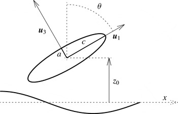
We consider an axially symmetric particle immersed in an incompressible Newtonian fluid, moving close to an elastic membrane. The fluid is assumed to have the same dynamic viscosity $\unicode[STIX]{x1D702}$ on both sides of the membrane. As an example, we will focus later on a prolate spheroidal particle as shown in figure 1. The position of the centre of the particle is $\boldsymbol{r}_{0}$ , while its orientation is described by the unit vector $\boldsymbol{u}_{1}$ pointing along the symmetry axis. The laboratory frame is spanned by the basis vectors $\{\boldsymbol{e}_{x},\boldsymbol{e}_{y},\boldsymbol{e}_{z}\}$ .

We denote by $z_{0}$ the vertical distance separating the centre of the particle from the undisplaced membrane located at the plane $z=0$ and extended infinitely in the horizontal plane  $xy$ . It is convenient to introduce the body-fixed frame of reference, formed by the three basis vectors $\{\boldsymbol{u}_{1},\boldsymbol{u}_{2},\boldsymbol{u}_{3}\}$ . The unit vector $\boldsymbol{u}_{2}$ is parallel to the undisplaced membrane and perpendicular to the particle axis, and $\boldsymbol{u}_{3}$ completes the orthonormal basis. We define $\unicode[STIX]{x1D703}$ as the angle between $\boldsymbol{u}_{1}$ and $\boldsymbol{e}_{z}$ such that $\cos \unicode[STIX]{x1D703}=\boldsymbol{e}_{z}\boldsymbol{\cdot }\boldsymbol{u}_{1}$ . The basis vectors in the particle frame are then given by $\boldsymbol{u}_{2}=(\boldsymbol{e}_{z}\times \boldsymbol{u}_{1})/|\boldsymbol{e}_{z}\times \boldsymbol{u}_{1}|$ and $\boldsymbol{u}_{3}=\boldsymbol{u}_{1}\times \boldsymbol{u}_{2}$ .

Figure 1.

Illustration of a spheroidal particle located at $z=z_{0}$ above an elastic cell membrane. The short and long axes are denoted by $a$ and $c$ , respectively. The unit vector $\boldsymbol{u}_{1}$ is pointing along the spheroid symmetry axis and $\boldsymbol{u}_{2}$ is the unit vector perpendicular to the plane of the figure. The unit vector $\boldsymbol{u}_{3}$ is defined to be orthogonal to both $\boldsymbol{u}_{1}$ and $\boldsymbol{u}_{2}$ .

In the inertia-free regime of motion, the fluid dynamics is governed by the stationary incompressible Stokes equations

where $\boldsymbol{v}$ is the fluid velocity, $p$ is the pressure field and $\boldsymbol{f}$ is the force density acting on the fluid due to the presence of the particle. We omit the unsteady term in the Stokes equations, since in realistic situations it leads to a negligible contribution to the mobility corrections (Daddi-Moussa-Ider et al. Reference Daddi-Moussa-Ider, Guckenberger and Gekle2016a ). For a discussion accounting for the unsteady term in the bulk flow, see recent work by Felderhof (Reference Felderhof2013). The flow $\boldsymbol{v}(\boldsymbol{r})$ may be superposed with an arbitrary external flow $\boldsymbol{v}_{0}(\boldsymbol{r})$ being a solution to the homogeneous Stokes equations in the absence of the particle.

Consider now a colloidal particle near the membrane. The total force $\boldsymbol{F}$ , torque $\boldsymbol{T}$ and stresslet (symmetric force dipole) $\boldsymbol{S}$ are linearly related to the velocities (translational $\boldsymbol{V}$ and angular $\unicode[STIX]{x1D734}$ ) of the particle relative to an external flow by the generalised friction tensor (Kim & Karrila Reference Kim and Karrila2013)

with $\boldsymbol{v}_{0}=\boldsymbol{v}_{0}(\boldsymbol{r}_{0})$ , the vorticity $\unicode[STIX]{x1D74E}_{0}=(1/2)\unicode[STIX]{x1D735}\times \boldsymbol{v}_{0}(\boldsymbol{r}_{0})$ and the rate of strain $\boldsymbol{E}_{0}=\overline{\unicode[STIX]{x1D735}\boldsymbol{v}_{0}}(\boldsymbol{r}_{0})$ of the external flow (the bar denotes the symmetric and traceless part of the velocity gradient).

A complementary relation defines the generalised mobility tensor

Upon examining (2.3) and (2.4), we note that the $6\times 6$ mobility tensor $\unicode[STIX]{x1D741}$ is the inverse of the friction tensor $\unicode[STIX]{x1D73B}$

Relations between other elements of the generalised mobility and friction tensors may be found directly from (2.3) and (2.4). These are general properties of Stokes flows following from the linearity of the governing equations. Finding an explicit form of these tensors requires the solution of Stokes equations (2.1) and (2.2) with appropriate boundary conditions on the confining interfaces. Since we aim at computing the particle mobility nearby a membrane endowed with surface elasticity and bending resistance, a relevant model for the membrane dynamics needs to be introduced at this point.

The Skalak model (Skalak et al. Reference Skalak, Tozeren, Zarda and Chien1973) is well established and commonly used to represent RBC membranes (Freund Reference Freund2014). The elastic properties of the interface are characterised by two moduli: elastic shear modulus $\unicode[STIX]{x1D705}_{S}$ and area dilatation modulus $\unicode[STIX]{x1D705}_{A}$ . Resistance towards bending has been further included following the model of Helfrich (Reference Helfrich1973) with the associated bending modulus $\unicode[STIX]{x1D705}_{B}$ . In this approach, the linearised tangential and normal traction jumps across the membrane are related to the membrane displacement field $\boldsymbol{h}$ at $z=0$ and the dilatation $\unicode[STIX]{x1D716}$ by (Daddi-Moussa-Ider et al. Reference Daddi-Moussa-Ider, Guckenberger and Gekle2016a )

where $[f]:=f(z=0^{+})-f(z=0^{-})$ denotes the jump of the quantity $f$ across the membrane. The dilatation $\unicode[STIX]{x1D716}:=\unicode[STIX]{x2202}_{x}h_{x}+\unicode[STIX]{x2202}_{y}h_{y}$ is the trace of the strain tensor. The Skalak parameter is defined as $C:=\unicode[STIX]{x1D705}_{A}/\unicode[STIX]{x1D705}_{S}$ . Here $\unicode[STIX]{x1D6E5}_{\Vert }:=\unicode[STIX]{x2202}_{x}^{2}+\unicode[STIX]{x2202}_{y}^{2}$ is the Laplace–Beltrami operator along the membrane. The components $\unicode[STIX]{x1D70E}_{z\unicode[STIX]{x1D6FC}}$ of the stress tensor in the fluid are expressed in a standard way by $\unicode[STIX]{x1D70E}_{z\unicode[STIX]{x1D6FC}}=-p\unicode[STIX]{x1D6FF}_{z\unicode[STIX]{x1D6FC}}+\unicode[STIX]{x1D702}(\unicode[STIX]{x2202}_{\unicode[STIX]{x1D6FC}}v_{z}+\unicode[STIX]{x2202}_{z}v_{\unicode[STIX]{x1D6FC}})$ for $\unicode[STIX]{x1D6FC}\in \{x,y,z\}$ (Kim & Karrila Reference Kim and Karrila2013).

The membrane displacement $\boldsymbol{h}$ and the fluid velocity $\boldsymbol{v}$ are related by the no-slip boundary condition at the undisplaced membrane, which in Fourier space takes the form

with $\unicode[STIX]{x1D714}$ being the characteristic frequency of forcing in the system. The frequency-dependent elastic deformation effects are characterised by two dimensionless parameters, as described in Daddi-Moussa-Ider et al. (Reference Daddi-Moussa-Ider, Guckenberger and Gekle2016a )

Further details of the derivation of $\unicode[STIX]{x1D6FD}$ and $\unicode[STIX]{x1D6FD}_{B}$ can be found in appendix A. The effects of shear resistance and area dilatation are thus captured by $\unicode[STIX]{x1D6FD}$ , while $\unicode[STIX]{x1D6FD}_{B}$ describes the bending resistance of the membrane. In the steady case for which $\unicode[STIX]{x1D6FD}=\unicode[STIX]{x1D6FD}_{B}=0$ , corresponding to a vanishing frequency or to an infinitely stiff membrane, we expect to recover the results for a hard no-slip wall.

In the case of periodic forcing or time-dependent deformation of the membrane, the quantity of interest is the frequency-dependent mobility tensor. Our aim in this work is to find all the components of $\unicode[STIX]{x1D741}(\unicode[STIX]{x1D714})$ for an axisymmetric particle close to an elastic membrane. Accordingly, due to the presence of the interface, the near-membrane mobility will then have a correction on top of the bulk mobility $\unicode[STIX]{x1D741}_{0}$ ,

stemming from the interaction of the flow created by the particle with the boundary. To determine the form of $\unicode[STIX]{x1D741}(\unicode[STIX]{x1D714})$ in an approximate manner, we use the results by Lisicki et al. (Reference Lisicki, Cichocki and Wajnryb2016) valid for a hard no-slip wall and generalize them to the case of an elastic membrane. Their idea is based on a multipole expansion (Cichocki et al. Reference Cichocki, Jones, Kutteh and Wajnryb2000) of the flow field around an axially symmetric particle close to a boundary, with a corresponding expansion of the force distribution on its surface. If the particle is sufficiently far away from the wall, they have shown that the dominant correction to its friction matrix can be viewed as an interaction between the centre of the particle and its hydrodynamic image. They provide explicit expressions for the elements of the friction tensor for all types of motion (translation, rotation and coupling terms) which yields the corrected mobility tensor upon inversion. The same route may be followed for a membrane, provided that the form of the Green’s tensor for the system is known.

A general Stokes flow can be constructed using the Green’s function $\boldsymbol{\{}(\boldsymbol{r},\boldsymbol{r}^{\prime })$ being the solution of (2.1) and (2.2) subject to a time-dependent point force $\boldsymbol{f}(r)=\boldsymbol{F}(t)\unicode[STIX]{x1D6FF}(\boldsymbol{r}-\boldsymbol{r}^{\prime })$ with the appropriate boundary conditions on the membrane. In an unbounded fluid, the Green’s tensor is the Oseen tensor (Kim & Karrila Reference Kim and Karrila2013) $\boldsymbol{\{}_{0}(\boldsymbol{r},\boldsymbol{r}^{\prime })=\boldsymbol{\{}_{0}(\boldsymbol{r}-\boldsymbol{r}^{\prime })$ , with $\boldsymbol{\{}_{0}(\boldsymbol{r})=(\mathbf{1}+\boldsymbol{r}\boldsymbol{r}/r^{2})/(8\unicode[STIX]{x03C0}\unicode[STIX]{x1D702}r)$ and $r:=|\boldsymbol{r}|$ . In the presence of boundaries, the Green’s tensor contains the extra term $\unicode[STIX]{x1D6AB}\boldsymbol{\{}$ describing the flow reflected from the membrane, so that $\boldsymbol{\{}=\boldsymbol{\{}_{0}+\unicode[STIX]{x1D6AB}\boldsymbol{\{}$ .

The exact Green’s function for a point force close to a membrane has recently been computed in Daddi-Moussa-Ider et al. (Reference Daddi-Moussa-Ider, Guckenberger and Gekle2016a ). For the resolution of (2.1) and (2.2) with a point force acting at $\boldsymbol{r}_{0}=(0,0,z_{0})$ , the two-dimensional Fourier transform in the $xy$ plane was used to solve the resulting equations with accordingly transformed boundary conditions. The procedure has been previously described in detail and therefore we only list the main steps for the determination of the Green’s tensor in appendix A of this work.

3 Near-membrane mobility tensors

We search for the near-membrane mobility tensor, $\unicode[STIX]{x1D741}(\unicode[STIX]{x1D714})=\unicode[STIX]{x1D741}_{0}+\unicode[STIX]{x1D6AB}\unicode[STIX]{x1D741}(\unicode[STIX]{x1D714})$ by calculating the leading-order correction to the bulk mobility. To this end, we follow the route outlined in a recent contribution by Lisicki et al. (Reference Lisicki, Cichocki and Wajnryb2016) who derived analytic expressions for the friction tensor of an axially symmetric particle in the presence of a hard no-slip wall. The friction tensor, similarly to the mobility tensor, can be split into the bulk and the correction term

The final expressions for the corrected friction tensor involve elements of the bulk friction tensor of the particle, and the distance- and orientation-dependent (derivatives of) the appropriate Green’s function. For the hard no-slip wall treated in Lisicki et al. (Reference Lisicki, Cichocki and Wajnryb2016) the latter is the Blake tensor (Blake Reference Blake1971) while in the present case the frequency-dependent Green’s functions from Daddi-Moussa-Ider et al. (Reference Daddi-Moussa-Ider, Guckenberger and Gekle2016a ) are employed. The expressions for the friction tensor with a general Green’s function read (Lisicki et al. Reference Lisicki, Cichocki and Wajnryb2016)

where the directional tensors $\unicode[STIX]{x1D65C}$ are defined by

Here, $\unicode[STIX]{x1D6AB}\boldsymbol{\{}^{\unicode[STIX]{x1D6FE}\unicode[STIX]{x1D6FF}}$ are the multipole elements of the Green’s integral operator which will be derived below. Further, $\unicode[STIX]{x1D6FE},\unicode[STIX]{x1D6FF}\in \{t,r,d\}$ and $a=1$ for $tt$ , $a=2$ for $(tr,rt,td,dt)$ and $a=3$ for $(dr,rd,rr,dd)$ parts. In (3.2)–(3.5) it should be understood that the tensors are appropriately contracted to yield second-order tensor corrections.

We now apply this result to our system. Our goal is to obtain explicit expressions for the mobility tensors for an axially symmetric particle in the presence of a membrane in terms of its bulk mobilities. This can be done in two steps.

Firstly, we invert the friction relations (3.2)–(3.5), as detailed in appendix B, to obtain analogous relations for the mobilities:

These expressions allow straightforward computation of the near-membrane mobilities for axisymmetric particles of arbitrary shape if their bulk mobilities are known, either numerically or analytically. Compared to a numerical inversion of the friction tensor, which in principle would be preferable as it avoids the possibility of negative mobilities (Lisicki et al. Reference Lisicki, Cichocki and Wajnryb2016), this approach has the advantage that explicit analytical expressions for the mobility can be obtained.

Remarkably, the final formulae include only one bulk characteristic of the particle, namely the tensors $\unicode[STIX]{x1D741}_{0}^{rd}$ and $\unicode[STIX]{x1D741}_{0}^{dr}$ which describe the rotational motion of the particle in response to elongational flow. This form follows from the particular symmetries of an axially symmetric particle with inversional symmetry ( $\boldsymbol{u}_{1}\leftrightarrow -\boldsymbol{u}_{1}$ ).

Secondly, to obtain the directional tensors $\unicode[STIX]{x1D65C}$ , we consider a general Green’s tensor $\boldsymbol{\{}(\boldsymbol{r},\boldsymbol{r}^{\prime })=\boldsymbol{\{}_{0}(\boldsymbol{r}-\boldsymbol{r}^{\prime })+\unicode[STIX]{x1D6AB}\boldsymbol{\{}(\boldsymbol{r},\boldsymbol{r}^{\prime })$ and a body placed at $\boldsymbol{r}_{0}$ with a force distribution $\boldsymbol{f}(\boldsymbol{r})$ on its surface. The flow at a point $\boldsymbol{r}$ due to this forcing may be written as the integral equation

with the integral performed over the surface of the body. The idea of the derivation of the correction is to find, given the force density, the flow incident on the particle itself due to the presence of an interface. Thus we consider (3.11) with only the membrane interaction part $\unicode[STIX]{x1D6AB}\boldsymbol{\{}(\boldsymbol{r},\boldsymbol{r}^{\prime })$ of the Green’s tensor and expand it in both arguments around $\boldsymbol{r}=\boldsymbol{r}^{\prime }=\boldsymbol{r}_{0}$ . The integrals of the subsequent terms on the right-hand side reproduce the force multipole moments, while the expansion of the left-hand side yields the multipole expansion of the flow field. By matching the relevant multipoles, we find explicit expressions for the $\unicode[STIX]{x1D6AB}\boldsymbol{\{}^{\unicode[STIX]{x1D6FE}\unicode[STIX]{x1D6FF}}$ , with $\unicode[STIX]{x1D6FE},\unicode[STIX]{x1D6FF}\in \{t,r,d\}$ , as described in Lisicki et al. (Reference Lisicki, Cichocki and Wajnryb2016). The resulting formulae are

where $\unicode[STIX]{x1D716}_{\unicode[STIX]{x1D6FC}\unicode[STIX]{x1D707}\unicode[STIX]{x1D708}}$ is the Levi-Civita tensor and the symbol   denotes the symmetric and traceless part with respect to indices $\unicode[STIX]{x1D6FC},\unicode[STIX]{x1D6FD}$ . Explicitly, the reductions for an arbitrary third- and fourth-order traceless tensor read

The prime denotes a derivative with respect to the second argument. We note that the tensors $\unicode[STIX]{x1D6AB}\boldsymbol{\{}^{dr,rd,dd}$ are traceless due to the incompressibility of the fluid, and therefore the trace need not be subtracted in the procedure of symmetrisation. We further remark that (3.12) through (3.20) involves differentiations and elementary operations that are well defined for complex quantities, and hence lead to convergent limits.

It is most natural to consider the correction in the reference frame of the particle, spanned by the three unit basis vectors $\{\boldsymbol{u}_{1},\boldsymbol{u}_{2},\boldsymbol{u}_{3}\}$ . In this frame, the mobility tensors of an axisymmetric particle have the form

for translational and rotational motion, while the translation–rotation coupling tensor reads

The rotation–translation coupling tensor $\unicode[STIX]{x1D6AB}\unicode[STIX]{x1D741}^{rt}$ is obtained by simply taking the transpose of the translation–rotation coupling tensor given above. (See supplemental material available at https://doi.org/10.1017/jfm.2016.739 for the frequency-dependent mobility corrections expressed in the laboratory frame).

4 Boundary integral method

Here we introduce the boundary integral method (Pozrikidis Reference Pozrikidis2001) used to numerically compute the mobility tensor of a truly extended spheroidal particle. The method is perfectly suited for treating three-dimensional problems with complex, deforming boundaries such as RBC membranes in the Stokes regime (Zhao & Shaqfeh Reference Zhao and Shaqfeh2011; Zhu Reference Zhu2014). In order to solve for the particle motion, given an applied force or torque, we combine a completed double layer boundary integral method (CDLBIM) (Power & Miranda Reference Power and Miranda1987) with the classical BIM (Zhao, Shaqfeh & Narsimhan Reference Zhao, Shaqfeh and Narsimhan2012). The resulting equations are then discretised and transformed into a system of algebraic equations as detailed in (Daddi-Moussa-Ider et al. Reference Daddi-Moussa-Ider, Guckenberger and Gekle2016b ; Guckenberger et al. Reference Guckenberger, Schraml, Chen, Leonetti and Gekle2016).

For the numerical determination of the particle mobility components, a harmonic force $\boldsymbol{F}(t)=\boldsymbol{A}\text{e}^{\text{i}\unicode[STIX]{x1D714}_{0}t}$ or torque $\boldsymbol{T}(t)=\boldsymbol{B}\text{e}^{\text{i}\unicode[STIX]{x1D714}_{0}t}$ is applied at the particle surface. After a short transient evolution, the particle linear and angular velocities can be described as $\boldsymbol{V}(t)=\boldsymbol{C}\text{e}^{\text{i}(\unicode[STIX]{x1D714}_{0}t+\unicode[STIX]{x1D6FF}_{t})}$ and $\unicode[STIX]{x1D734}(t)=\boldsymbol{D}\text{e}^{\text{i}(\unicode[STIX]{x1D714}_{0}t+\unicode[STIX]{x1D6FF}_{r})}$ respectively. The amplitudes and phase shifts can be determined accurately by fitting the numerically recorded velocities using the trust region method (Conn, Gould & Toint Reference Conn, Gould and Toint2000). In the laboratory frame, the components $\unicode[STIX]{x1D707}_{\unicode[STIX]{x1D6FC}\unicode[STIX]{x1D6FD}}^{tt}$ and $\unicode[STIX]{x1D707}_{\unicode[STIX]{x1D6FC}\unicode[STIX]{x1D6FD}}^{rt}$ of the mobility are determined for a torque-free particle as

For a force-free particle, the components $\unicode[STIX]{x1D707}_{\unicode[STIX]{x1D6FC}\unicode[STIX]{x1D6FD}}^{tr}$ and $\unicode[STIX]{x1D707}_{\unicode[STIX]{x1D6FC}\unicode[STIX]{x1D6FD}}^{rr}$ are obtained from

5 Spheroid close to a membrane: theoretical and numerical results

In this section, we present a comparison of our theoretical results to numerical simulations using the example of a prolate spheroidal particle. To begin with, we discuss the bulk mobility of a spheroid. Further on, we show the explicit form of the correction, and finally compare the components of the corrected mobility matrix to numerical simulations.

The bulk translational and rotational mobility tensors of a general axisymmetric particle have the form

The third-order tensors $\unicode[STIX]{x1D741}_{0}^{rd}$ and $\unicode[STIX]{x1D741}_{0}^{dr}$ have the Cartesian components

where, following from the Lorentz reciprocal theorem (Kim & Karrila Reference Kim and Karrila2013)

Note that due to the axial and inversional symmetry in bulk, we have $\unicode[STIX]{x1D741}_{0}^{tr}=\unicode[STIX]{x1D741}_{0}^{rt}=0$ and $\unicode[STIX]{x1D741}_{0}^{td}=\unicode[STIX]{x1D741}_{0}^{dt}=0$ .

For a prolate spheroidal particle of eccentricity $e$ , analytical results are available and the bulk mobility coefficients are given by Kim & Karrila (Reference Kim and Karrila2013, table 3.4)

where $a$ and $c$ are the short and long axis of the spheroid and

To obtain the final ingredient $\unicode[STIX]{x1D707}^{rd}$ , we observe from the definitions in (2.3) and (2.4) that $\unicode[STIX]{x1D707}_{\unicode[STIX]{x1D6FC}\unicode[STIX]{x1D6FD}\unicode[STIX]{x1D6FE}}^{rd}=\unicode[STIX]{x1D707}_{\unicode[STIX]{x1D6FC}\unicode[STIX]{x1D6FF}}^{rr}\unicode[STIX]{x1D701}_{\unicode[STIX]{x1D6FF}\unicode[STIX]{x1D6FD}\unicode[STIX]{x1D6FE}}^{rd}$ and $\unicode[STIX]{x1D707}_{\unicode[STIX]{x1D6FC}\unicode[STIX]{x1D6FD}\unicode[STIX]{x1D6FE}}^{dr}=-\unicode[STIX]{x1D701}_{\unicode[STIX]{x1D6FC}\unicode[STIX]{x1D6FD}\unicode[STIX]{x1D6FF}}^{dr}\unicode[STIX]{x1D707}_{\unicode[STIX]{x1D6FF}\unicode[STIX]{x1D6FE}}^{rr}$ , leading to

The component $rd$ of the friction tensor is (Kim & Karrila Reference Kim and Karrila2013)

Therefore we obtain the $rd$ coefficient of the mobility tensor

Having introduced the bulk hydrodynamic mobilities of a spheroid, we turn our attention to the membrane correction which in the frame of the particle can be written as in (3.23) and (3.24). We find that the corrections to the translational mobilities as given in general form in (3.7) can, for a spheroid, be written in closed form as

and $\unicode[STIX]{x0394}\unicode[STIX]{x1D707}_{13}^{tt}=\unicode[STIX]{x0394}\unicode[STIX]{x1D707}_{31}^{tt}$ . Thus they have the desired symmetry of (3.23). Expressions for $P(\unicode[STIX]{x1D6FD},\unicode[STIX]{x1D6FD}_{B})=P_{S}(\unicode[STIX]{x1D6FD})+P_{B}(\unicode[STIX]{x1D6FD}_{B})$ and $Q(\unicode[STIX]{x1D6FD},\unicode[STIX]{x1D6FD}_{B})=Q_{S}(\unicode[STIX]{x1D6FD})+Q_{B}(\unicode[STIX]{x1D6FD}_{B})$ are provided explicitly in appendix C.

For the translation–rotation coupling, the non-vanishing mobility corrections as given by (3.8), can be cast in the frame of the particle as

where $M$ and $N$ are now functions of the parameters $\unicode[STIX]{x1D6FD}$ and $\unicode[STIX]{x1D6FD}_{B}$ , and can likewise be decomposed into shearing and bending contributions. The dependence on the bulk $rd$ mobility $\unicode[STIX]{x1D706}$ is explicitly separated out.

Figure 2.

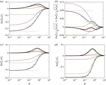
The scaled translational mobility correction components versus the scaled frequency. The spheroid is located above the membrane at $z_{0}=2c$ inclined at an angle $\unicode[STIX]{x1D703}=\unicode[STIX]{x03C0}/3$ from the vertical. The analytical predictions of the real and imaginary parts of the translational mobility corrections are shown as dashed and solid lines, respectively. The corrections due to shearing and bending are shown respectively in green (bright grey in a black and white printout) and red (dark grey in a black and white printout). Horizontal dotted lines represent the hard-wall limits from Lisicki et al. (Reference Lisicki, Cichocki and Wajnryb2016). BIM simulations are marked as squares and circles for the real and imaginary parts, respectively. For the membrane parameters we take a reduced bending modulus $E_{B}:=\unicode[STIX]{x1D705}_{B}/(c^{2}\unicode[STIX]{x1D705}_{S})=2/3$ and the Skalak parameter $C=1$ .

Finally, considering the rotational part as stated by (3.10), the non-vanishing components of the mobility correction in the frame of the particle can conveniently be cast in the following forms

and with $\unicode[STIX]{x0394}\unicode[STIX]{x1D707}_{13}^{rr}=\unicode[STIX]{x0394}\unicode[STIX]{x1D707}_{31}^{rr}$ . All the functions depend on $(\unicode[STIX]{x1D6FD},\unicode[STIX]{x1D6FD}_{B})$ and are decomposed into bending and shearing parts in appendix C. In addition, the functions $C$ , $D$ and $H$ depend on the coefficient $\unicode[STIX]{x1D706}$ .

It can be seen that the mobility corrections for an axisymmetric particle in their dominant terms possess a simple angular structure. The latter stems from the contraction of the particle friction tensors (which have an axial symmetry, dictated by their shape, with respect to the body axis) with the vertical multipole components of the Blake tensor (which have the same structure but with respect to a different axis, i.e. the vertical direction). This contraction requires transformation of corresponding tensors into the common frame of reference, which generates simple polynomials in sine and cosine functions of the inclination angle as discussed in Lisicki et al. (Reference Lisicki, Cichocki and Wajnryb2016).

In the following, we shall present a comparison between these analytical predictions and numerical simulations using the BIM, presented in § 4. We consider a prolate spheroid of aspect ratio $p:=c/a=2$ , inclined at an angle $\unicode[STIX]{x1D703}=\unicode[STIX]{x03C0}/3$ to the $z$ axis, positioned at $z_{0}=2c$ above a planar elastic membrane. For the membrane, we take a reduced bending modulus $E_{B}:=c^{2}\unicode[STIX]{x1D705}_{S}/\unicode[STIX]{x1D705}_{B}=3/2$ for which the characteristic frequencies $\unicode[STIX]{x1D6FD}$ and $\unicode[STIX]{x1D6FD}_{B}^{3}$ have the same order of magnitude. The Skalak parameter is $C=1$ . Corresponding data showing the effect of the inclination angle and the reduced bending modulus can be found in the Supporting Information. Our analytical predictions are applicable for large and moderate membrane–particle distances for which $c/z_{0}\sim O(1)$ where we find good agreement with numerical simulations.

Henceforth, the mobility corrections will be scaled by the associated bulk values. For diagonal terms, we choose the corresponding diagonal elements, namely $\unicode[STIX]{x1D707}_{\Vert }^{t,r}$ for $\unicode[STIX]{x1D707}_{11}^{t,r}$ and $\unicode[STIX]{x1D707}_{\bot }^{t,r}$ for $\unicode[STIX]{x1D707}_{22,33}^{t,r}$ . For non-diagonal terms, we use an appropriate combination of bulk mobilities, that is $\sqrt{\unicode[STIX]{x1D707}_{\Vert }^{t,r}\unicode[STIX]{x1D707}_{\bot }^{t,r}}$ for translations and rotations. The translation–rotation coupling tensors are scaled by $\sqrt{\unicode[STIX]{x1D707}_{\bot }^{t}\unicode[STIX]{x1D707}_{\bot }^{r}}$ .

Figure 3.

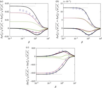
The scaled coupling mobility corrections versus the scaled frequency. Black and blue symbols refer to the $tr$ and $rt$ components, respectively, obtained from BIM simulations. The other colours are the same as in figure 2.

Figure 4.

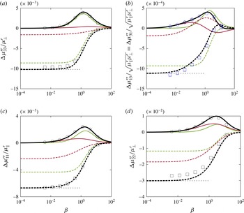
The scaled rotational mobility correction component versus the scaled frequency. Black and blue symbols refer to the 13 and 31 components, respectively, obtained from BIM simulations. The colour code is the same as in figure 2.

In figure 2 we compare the components of the translational mobility calculated from (5.13)–(5.16) with those obtained from BIM simulations. For the diagonal components we observe that the real part of the complex mobility corrections is monotonically increasing with frequency. The imaginary part exhibits a non-monotonic bell-shaped dependence on frequency that peaks around $\unicode[STIX]{x1D6FD}\sim 1$ . The off-diagonal components 13 and 31 show a more complex dependence on frequency. In the vanishing frequency limit, we recover the corrections near a hard wall with stick boundary conditions recently calculated by Lisicki et al. (Reference Lisicki, Cichocki and Wajnryb2016). We further remark that for the present inclination of $\unicode[STIX]{x1D703}=\unicode[STIX]{x03C0}/3$ the components 33 and 13 are principally determined by bending resistance whereas the shearing effect is more pronounced in the components 11 and 22. A very good agreement is obtained between analytical predictions and numerical simulations for all components over the entire range of frequencies.

By examining the off-diagonal component 31 shown in figure 2(b), it is clear that the shearing- and bending-related parts may have opposite contributions to the total translational mobility. This observed trend implies that upon exerting a force along $\boldsymbol{u}_{1}$ , there exists a drift motion along $\boldsymbol{u}_{3}$ , either away or towards the membrane, depending on the shearing and bending properties. In fact, for a membrane with bending-only resistance, such as a fluid vesicle, the spheroid is pushed away from the membrane in the same way as near a hard wall. On the other hand, for a membrane with shearing-only resistance, such as an artificial capsule, the motion is directed towards the membrane.

Figure 3 shows the corrections to the translation–rotation coupling mobility versus the scaled frequency computed from (5.17) and (5.19). We observe that bending resistance is essentially the dominant contributor to the coupling mobility. It can be shown that this trend is always the case regardless of spheroid orientation. The BIM simulation results are consistent with the fact that the $tr$ and $rt$ mobility tensors are the transpose of each other and a good agreement is obtained between analytical predictions and simulations. The coupling terms are generally very small compared to the relevant bulk quantities. This makes them somewhat more difficult to obtain precisely from the simulations which explains the small discrepancy notable in figure 3(a).

In figure 4 we present the corrections to the components of the rotational mobility tensor as calculated by (5.20)–(5.23) compared to the BIM simulations. We remark that the shearing contribution manifests itself in a more pronounced way for the rotational mobilities. Moreover, the correction to the rotational motion is less noticeable compared to the translational motion especially for the off-diagonal component. This observation can be explained by the fact that the rotational mobility corrections exhibit a faster decay with the distance from the membrane, scaling as $z_{0}^{-3}$ compared to $z_{0}^{-1}$ for translational motion. Again, a good agreement is obtained for the rotational mobility corrections between analytical predictions and numerical simulations.