1 Introduction
Interaction of objects with liquid–gas interfaces is relevant to a variety of applications in natural and industrial processes, e.g. water entry of solid objects (Vella & Metcalfe Reference Vella and Metcalfe2007; Aristoff & Bush Reference Aristoff and Bush2009; Ding et al. Reference Ding, Chen, Liu, Zhang, Gao and Lu2015), locomotion of insects on water (Bush & Hu Reference Bush and Hu2006), self-assembly of particles and fibres at fluid–fluid interface (Madivala, Fransaer & Vermant Reference Madivala, Fransaer and Vermant2009), mineral flotation (Ueda et al. Reference Ueda, Tanaka, Uemura and Iguchi2010; Liu, Evans & He Reference Liu, Evans and He2016), wet scrubbing (Jaworek et al. Reference Jaworek, Balachandran, Krupa, Kulon and Lackowski2006) and the design of water walking microrobots (Koh et al. Reference Koh, Yang, Jung, Jung, Son, Lee, Jablonski, Wood, Kim and Cho2015). One key factor in the object–interface interaction is the wettability of the object. Water entry of a hydrophobic sphere was found to easily give rise to an air cavity with a loud splash, while no air entrainment occurred in the water entry of a hydrophilic one at the same impact speed (Duez et al. Reference Duez, Ybert, Clanet and Bocquet2007). The effect of wettability is more important for small objects. The superhydrophobic legs of a water strider accounts for its effortless floating on the water surface (Gao & Jiang Reference Gao and Jiang2004), and even allows it to jump as high as several times its body length without piercing the water’s surface (Hu & Bush Reference Hu and Bush2010; Yang et al. Reference Yang, Son, Jablonski and Kim2016). Recent reviews of object–interface interaction can be found in Truscott, Epps & Belden (Reference Truscott, Epps and Belden2014) and Vella (Reference Vella2015).
To deepen our understanding of the role of wettability in the dynamic interaction between the object and the interface, we focus on the impact of a hydrophobic small sphere onto a liquid pool. The dynamics of the impacting sphere is expected to be determined by a group of dimensionless parameters, namely the Weber number
 $We$
(
 $=\unicode[STIX]{x1D70C}_{L}U_{0}^{2}D/\unicode[STIX]{x1D6FE}$
), the Bond number
 $Bo$
(
 $=\unicode[STIX]{x1D70C}_{L}gD^{2}/\unicode[STIX]{x1D6FE}$
), the Reynolds number
 $Re$
(
 $=\unicode[STIX]{x1D70C}_{L}U_{0}D/\unicode[STIX]{x1D707}$
), the density ratio of the sphere to the liquid
 $\unicode[STIX]{x1D706}_{\unicode[STIX]{x1D70C}}$
(
 $=\unicode[STIX]{x1D70C}_{S}/\unicode[STIX]{x1D70C}_{L}$
) and the wettability (represented by the contact angle
 $\unicode[STIX]{x1D703}$
), where
 $U_{0}$
is the impact velocity,
 $D$
and
 $\unicode[STIX]{x1D70C}_{S}$
the diameter and density of the sphere,
 $\unicode[STIX]{x1D70C}_{L}$
and
 $\unicode[STIX]{x1D707}$
the density and viscosity of the liquid and
 $\unicode[STIX]{x1D6FE}$
the surface tension coefficient. It has been experimentally observed by Lee & Kim (Reference Lee and Kim2008) that water entry of a superhydrophobic millimetre-sized sphere (
 $\unicode[STIX]{x1D703}\approx 154^{\circ }$
) exhibited rather distinct phenomena at a relatively low impact speed (
 $We\sim O(10^{1})$
and
 $Bo\sim O(10^{-1})$
). More specifically, the sphere could sink into the water, bounce back into the air or be entrapped at the water surface (and oscillate with capillary waves), which will be referred to hereafter as the regimes of sinking, bouncing and oscillating, respectively. The critical conditions for changes in flow regimes have also been theoretically analysed (Lee & Kim Reference Lee and Kim2008), and were shown to generally follow the same scaling law,
 $WeBo^{3/2}\sim \unicode[STIX]{x1D706}_{\unicode[STIX]{x1D70C}}^{-2}$
, e.g. for the transition from the sinking to the bouncing and that from the bouncing to the oscillating regime. There are not many reported numerical simulations for these flow–structure interaction problems involving dynamic wetting. Ji, Song & Yao (Reference Ji, Song and Yao2017) observed the occurrence of sinking and oscillating regimes in the simulation of impact of hydrophobic spheres with contact angle hysteresis onto a liquid–gas interface. Kintea et al. (Reference Kintea, Breitenbach, Thammanna Gurumurthy, Roisman and Tropea2016) numerically found that the penetration depth that a hydrophobic sphere at certain impact speed can reach before rebounding was proportional to
 $We$
. It is noteworthy that only spheres of particular wettability were considered in the previous studies. It remains unclear how the critical conditions for regime transition change with the wettability of the sphere, and in particular, what role the hydrophobicity plays in determining whether an object is entrapped at an interface after impact.
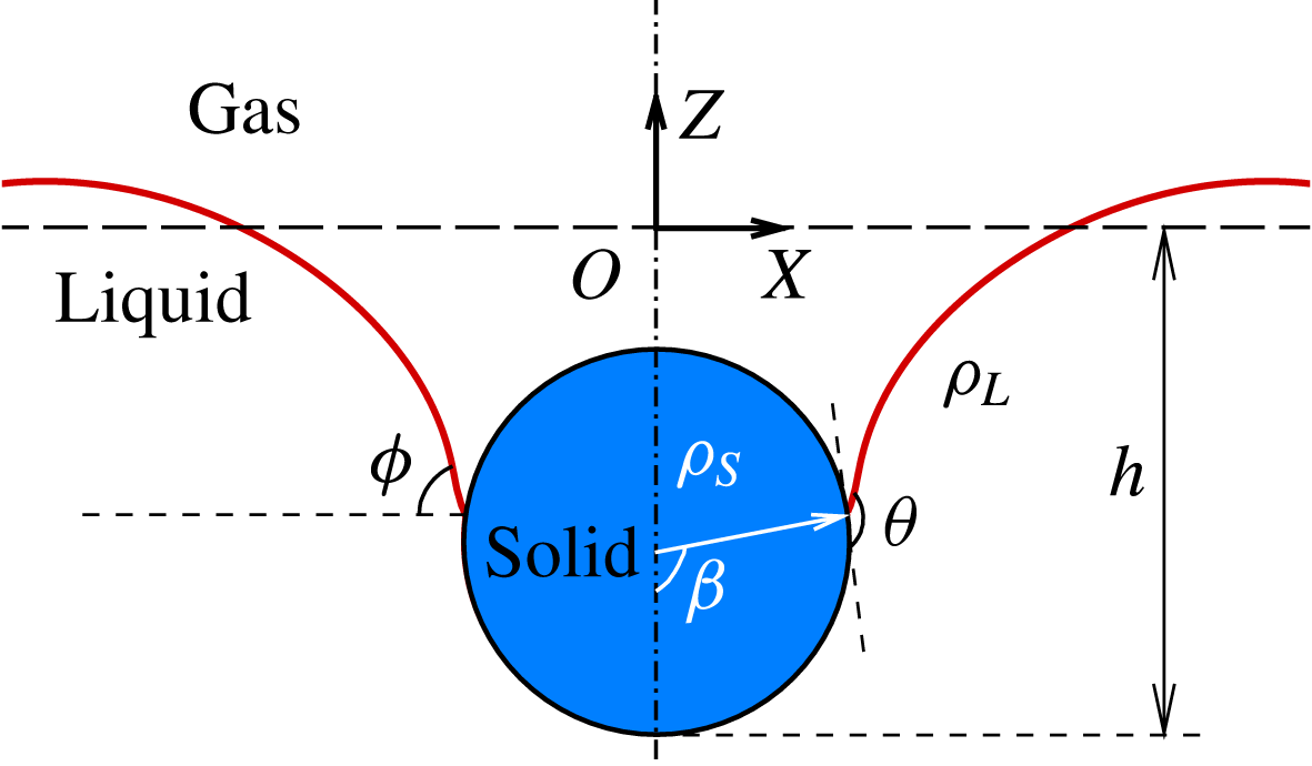
A sketch of a solid sphere impacting on a liquid pool. Solid curves represent the gas–liquid interface, and the long-dashed line denotes the undisturbed surface of the pool.

In this work, we numerically investigate the effect of hydrophobicity on the entrapment of an impacting sphere, which are denser than the liquid, at the liquid–gas interfaces (see figure 1). We consider the parameter space with
 $We\sim 4{-}50$
,
 $\unicode[STIX]{x1D706}_{\unicode[STIX]{x1D70C}}\sim 1{-}3$
,
 $\unicode[STIX]{x1D703}\sim 90^{\circ }{-}160^{\circ }$
and
 $Re\sim O(10^{3})$
. A diffuse-interface immersed-boundary (DIIB) method (Liu & Ding Reference Liu and Ding2015) is used for this purpose, accounting for the capillary force exerted on the sphere at the moving contact line (CL) (Liu, Gao & Ding Reference Liu, Gao and Ding2017). The numerical results provide not only the detailed information of the sphere–interface interaction after impact, but also the phase diagram with respect to
 $We$
versus
 $\unicode[STIX]{x1D703}$
(and
 $\unicode[STIX]{x1D706}_{\unicode[STIX]{x1D70C}}$
). We focus then on the mechanism leading to the entrapped spheres at the liquid–gas interface, such that the sphere neither penetrates the interface in its first descent nor bounces off from the interface when rebounding. To understand these two dynamic processes, we propose the respective scaling models, and verify them by comparing with numerical results. It shows that the models provide a good correlation among
 $We$
,
 $\unicode[STIX]{x1D706}_{\unicode[STIX]{x1D70C}}$
and
 $\unicode[STIX]{x1D703}$
with respect to the critical conditions at the onset of flow regime transition.
2 Methodology
We simulate the impact of a hydrophobic millimetric sphere onto a liquid pool using a DIIB method. The DIIB method allows us to simulate incompressible multiphase flows involving rigid objects of irregular shape and moving CLs on a Cartesian mesh (Liu & Ding Reference Liu and Ding2015), and has been extended to simulate fluid–structure interaction with dynamic wetting (Liu et al.
Reference Liu, Gao and Ding2017). The liquid–gas interface is represented by the volume fraction of the liquid,
 $C_{L}$
, the evolution of which is governed by,
 $$\begin{eqnarray}\frac{\unicode[STIX]{x2202}C_{L}}{\unicode[STIX]{x2202}t}+\unicode[STIX]{x1D735}\boldsymbol{\cdot }(\boldsymbol{u}C_{L})=\frac{1}{Pe}\unicode[STIX]{x1D6FB}^{2}\unicode[STIX]{x1D713},\end{eqnarray}$$
where the chemical potential is defined as
 $$\begin{eqnarray}\unicode[STIX]{x1D713}=C_{L}^{3}-1.5C_{L}^{2}+0.5C_{L}-C_{L}C_{S}(1-C_{L}-C_{S})-C_{n}^{2}\unicode[STIX]{x1D6FB}^{2}C_{l},\end{eqnarray}$$
and
 $C_{n}$
(
 $=\unicode[STIX]{x1D716}/D$
) is the Cahn number and
 $\unicode[STIX]{x1D716}$
is a measure of the thickness of diffuse interface.
 $C_{n}$
is set to
 $0.75\unicode[STIX]{x0394}x$
and Péclet number is set to
 $Pe=1/C_{n}$
, where
 $\unicode[STIX]{x0394}x$
is the mesh size of the Cartesian mesh. To simulate the motion of CLs on the curved substrate, a characteristic moving CL model (Lee & Kim Reference Lee and Kim2011; Liu & Ding Reference Liu and Ding2015) is employed to update
 $C_{L}$
in the CL region, according to the local normal direction and wettability of the sphere. The wettability of the sphere is represented by the static contact angle
 $\unicode[STIX]{x1D703}$
. The distribution of volume fraction of the solid,
 $C_{S}$
, is prescribed according to the position of the sphere. More details of numerical implementation can be found in Liu & Ding (Reference Liu and Ding2015) and Liu et al. (Reference Liu, Gao and Ding2017).
The code has been quantitatively validated for the dynamic behaviours of a superhydrophobic sphere impacting onto a water pool (Liu et al.
Reference Liu, Gao and Ding2017), by comparing with the experimental data of Lee & Kim (Reference Lee and Kim2008) with respect to the evolution of the position of sinking and bouncing spheres. The same code has also been used to simulate drop impact onto a curved substrate, and the numerical results compared favourably with experiments (Zhu et al.
Reference Zhu, Liu, Mu, Gao, Ding and Lu2017). In all of the calculations reported here, the water entry of the sphere is simulated in a domain of
 $5D\times 5D$
on a uniform Cartesian mesh. We have checked that the numerical results converged with the mesh refinement (
 $\unicode[STIX]{x0394}x=0.01D$
,
 $0.005D$
and
 $0.0025D$
), and thus choose
 $\unicode[STIX]{x0394}x=0.005D$
in the present study.
3 Results and discussion
Unless stated otherwise, we fix the Bond number to
 $Bo=0.48$
, the density ratio of solid to liquid to
 $\unicode[STIX]{x1D706}_{\unicode[STIX]{x1D70C}}=1.32$
and the density and viscosity ratio of gas to liquid to 0.001 and 0.018 respectively. The dimensionless time
 $\unicode[STIX]{x1D70F}$
(
 $=t\,U_{0}/D$
) is used to illustrate the time variation of numerical results. In the present study, the variation of
 $We$
is performed by changing the impact velocity, and thus we have
 $Re\propto \sqrt{We}$
.
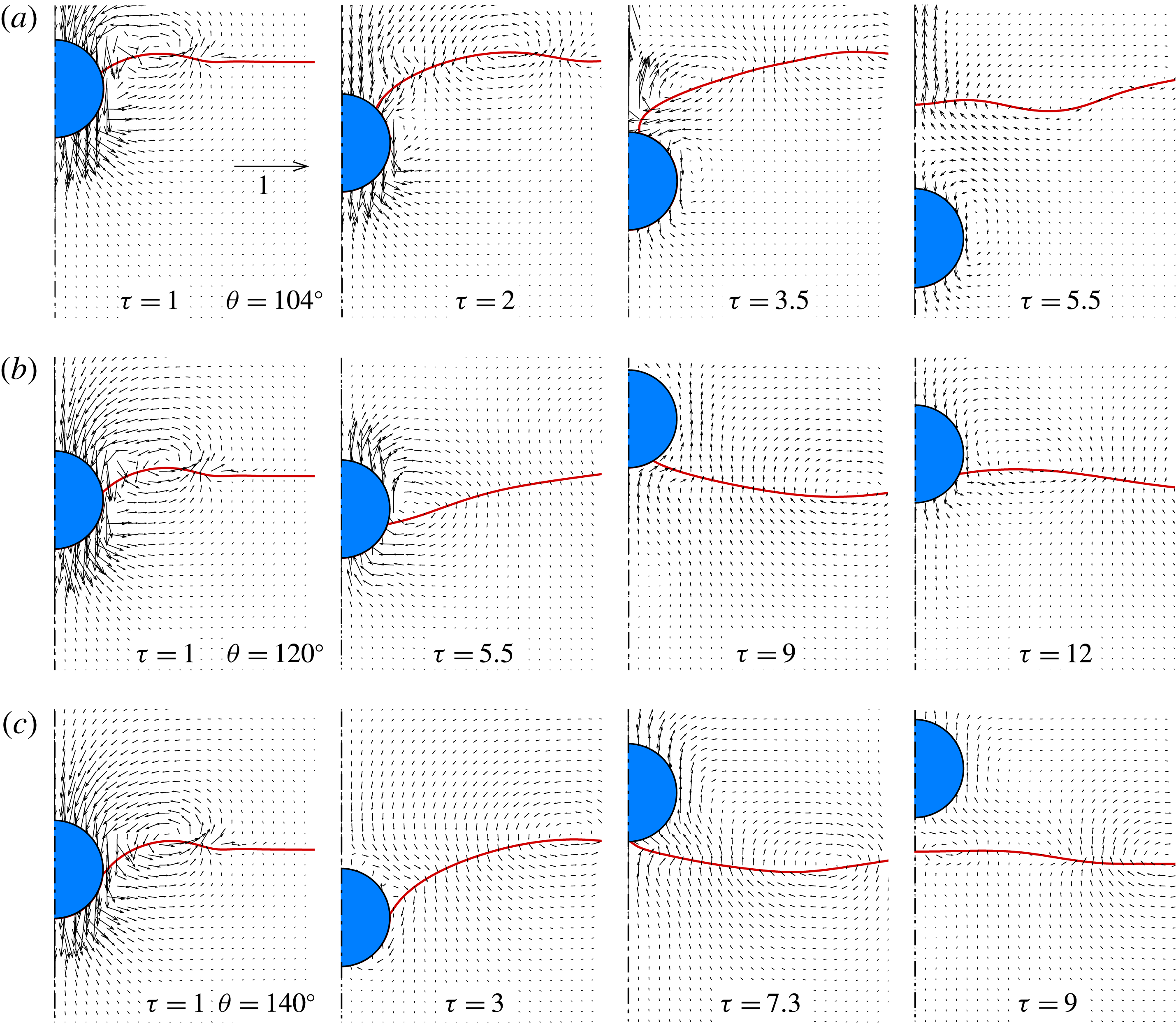
Illustration of impact dynamics of a hydrophobic sphere impacting onto a water pool at
 $We=10.2$
and
 $Re=1200$
, in terms of the liquid–gas interface and velocity vectors. Depending on the wettability, three regimes of impact are observed: sinking sphere (a and
 $\unicode[STIX]{x1D703}=104^{\circ }$
), oscillating sphere (b and
 $\unicode[STIX]{x1D703}=120^{\circ }$
) and bouncing sphere (c and
 $\unicode[STIX]{x1D703}=140^{\circ }$
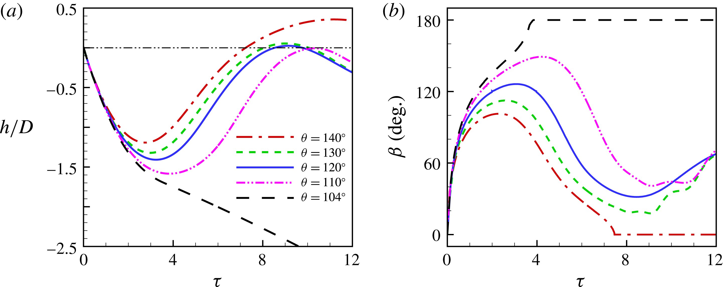
), respectively. The arrow in the top left panel denotes the reference velocity.

Results at
 $We=10.2$
,
 $Re=1200$
and various values of
 $\unicode[STIX]{x1D703}$
. (a) Time evolution of the displacement of the sphere, and
 $h=0$
(dash-dot-dotted line) denotes the undisturbed water surface. (b) Time evolution of the angular position of the CL in terms of
 $\unicode[STIX]{x1D6FD}$
(see figure 1).
 $\unicode[STIX]{x1D6FD}=0^{\circ }$
and
 $\unicode[STIX]{x1D6FD}=180^{\circ }$
correspond to the bouncing and sinking spheres, respectively.

3.1 Flow regimes
Figure 2 shows the flow features of the three flow regimes that occur in the water entry of a hydrophobic sphere at
 $We=10.2$
and
 $Re=1200$
, with respect to velocity vectors and interface evolution. When the hydrophobicity of the sphere is reduced, the flow regime changes from bouncing (
 $\unicode[STIX]{x1D703}=140^{\circ }$
) to oscillating (
 $\unicode[STIX]{x1D703}=120^{\circ }$
), and then to sinking (
 $\unicode[STIX]{x1D703}=104^{\circ }$
). Obviously, the wettability plays an important role in the dynamic interaction between the sphere and the gas–liquid interface. The sphere–interface interaction consists of two processes: sphere descending and sphere rebounding, characterized by the penetration depth
 $h$
and the CL position
 $\unicode[STIX]{x1D6FD}$
(see the definitions in figure 1). The flow regimes are determined by the outcome of these two processes, i.e. whether the sphere penetrates the interface in the first process and whether the sphere bounces from the interface in the second one. Figure 3 shows the time variation of
 $h$
and
 $\unicode[STIX]{x1D6FD}$
at
 $We=10.2$
,
 $Re=1200$
and
 $\unicode[STIX]{x1D703}$
ranging from
 $104^{\circ }$
to
 $140^{\circ }$
. In these cases,
 $\unicode[STIX]{x1D703}=110^{\circ }$
and
 $130^{\circ }$
approximately correspond to the boundaries of the oscillating regime. It is interesting to see that, despite of the difference in wettability, the highest position the oscillating spheres can reach is approximately the horizontal of the undisturbed water surface, i.e.
 $h=0$
. Moreover, the bouncing sphere also detaches from the liquid surface nearly at
 $h=0$
(see the snapshot at
 $\unicode[STIX]{x1D70F}=7.3$
in figure 2
c).
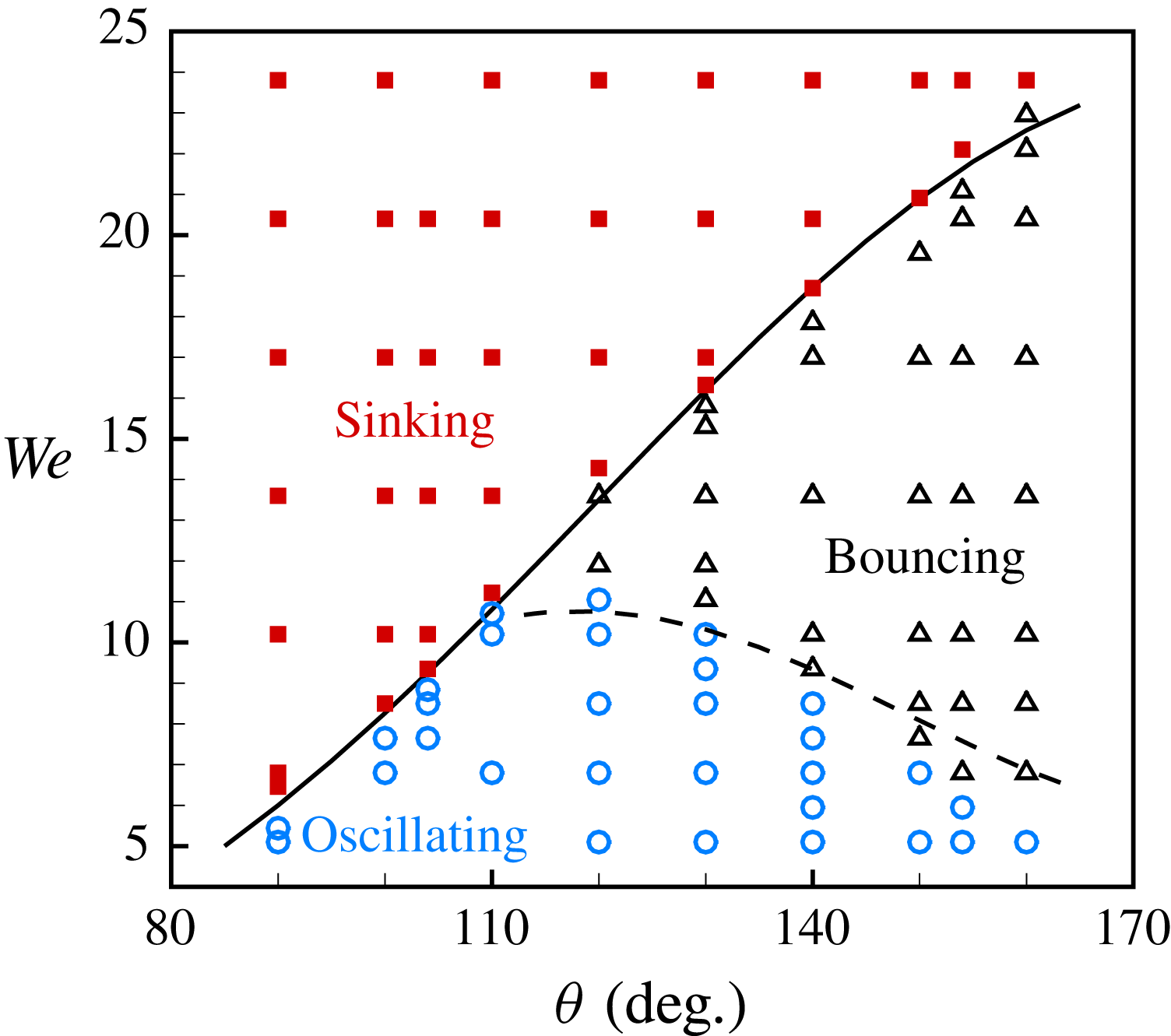
Phase diagram of a sphere impacting onto a liquid pool with respect to
 $We$
and
 $\unicode[STIX]{x1D703}$
, including the regimes of sinking ( ◼ ), bouncing (▵) and oscillating (◯). The solid line represents the theoretical analysis of (3.3) with a prefactor
 $k_{1}=13.9$
. The dashed line correspond to the prediction of (3.8) with a prefactor
 $k_{2}=31$
.

Phase diagram of a sphere impacting onto a liquid pool with respect to
 $WeBo^{3/2}$
and
 $\unicode[STIX]{x1D706}_{\unicode[STIX]{x1D70C}}^{2}$
for
 $\unicode[STIX]{x1D703}=154^{\circ }$
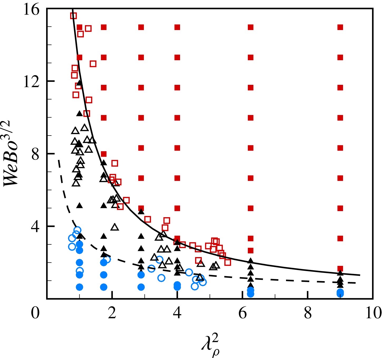
. The symbols of squares, triangles and circles represent the regimes of sinking, bouncing and oscillating, respectively. In particular, the empty symbols denote the experimental data of Lee & Kim (Reference Lee and Kim2008), and the filled ones represent our numerical results. The solid line represents the theoretical analysis of (3.3) with a prefactor
 $k_{1}=13.9$
, and the dashed line corresponds to the prediction of (3.8) with a prefactor
 $k_{2}=31$
.

Figure 4 shows the phase diagram of water entry of a sphere with respect to
 $We$
versus
 $\unicode[STIX]{x1D703}$
. The boundaries separating the three flow regimes assume a shape of reverse ‘
 $\unicode[STIX]{x1D706}$
’, with the intersection anchoring at
 $We\approx 12$
and
 $\unicode[STIX]{x1D703}\approx 110^{\circ }$
. The phase diagram can be firstly divided into the regions of sinking and non-sinking spheres according to the criterion for interface penetration. Then, the oscillating spheres can be further separated from the bouncing ones by the criterion for sphere bouncing. It is interesting to see that the bouncing spheres only occur with the sufficiently large contact angle (
 $\unicode[STIX]{x1D703}\geqslant 110^{\circ }$
). On the other hand, the sphere would not be entrapped at the interface unless the impact speed is sufficiently low (
 $We\leqslant 12$
). Figure 5 shows the phase diagram of the flow regimes obtained by numerical simulations at a fixed contact angle (
 $\unicode[STIX]{x1D703}=154^{\circ }$
) with respect to
 $WeBo^{3/2}$
versus
 $\unicode[STIX]{x1D706}_{\unicode[STIX]{x1D70C}}^{2}$
, along with the experimental data of Lee & Kim (Reference Lee and Kim2008). We note that the Bond number is fixed in the simulations (
 $Bo=0.48$
) while varied in the experiments. Despite the difference in the range of the parameters, the numerical results are in good agreement with the experimental ones with respect to the boundaries of the flow regimes. Clearly, in order to predict the regime boundaries of sphere entrapment, it is necessary to obtain the criteria for the onset of interface penetration and sphere bouncing respectively.
3.2 Capillary force
During the sphere–interface interaction, a capillary force is exerted on the sphere by the interface at the CL. The magnitude and direction of the capillary force depend on the wettability of the sphere and the CL position. It is easy to obtain the vertical component of the capillary force
 $F_{s}=2\unicode[STIX]{x03C0}R\unicode[STIX]{x1D6FE}\sin \unicode[STIX]{x1D6FD}\sin \unicode[STIX]{x1D719}$
(see figure 1), where
 $\unicode[STIX]{x1D719}$
is the angle that the interface interacts with the horizontal at the CL. Taking the geometric relation
 $\unicode[STIX]{x1D719}=\unicode[STIX]{x1D703}+\unicode[STIX]{x1D6FD}-\unicode[STIX]{x03C0}$
into account, we can get
 $$\begin{eqnarray}F_{s}=\unicode[STIX]{x03C0}R\unicode[STIX]{x1D6FE}[\cos (\unicode[STIX]{x1D703}+2\unicode[STIX]{x1D6FD})-\cos \unicode[STIX]{x1D703}].\end{eqnarray}$$
Therefore, the maximum (
 $F_{s+}$
) and minimum (
 $F_{s-}$
) values of the capillary force can be analytically derived with respect to
 $\unicode[STIX]{x1D6FD}$
, and
 $$\begin{eqnarray}\displaystyle \left.\begin{array}{@{}c@{}}\displaystyle F_{s+}=\unicode[STIX]{x03C0}R\unicode[STIX]{x1D6FE}(1-\cos \unicode[STIX]{x1D703}),\quad \text{at}~\unicode[STIX]{x1D6FD}=\unicode[STIX]{x03C0}-\frac{\unicode[STIX]{x1D703}}{2},\\ \displaystyle F_{s-}=-\unicode[STIX]{x03C0}R\unicode[STIX]{x1D6FE}(1+\cos \unicode[STIX]{x1D703}),\quad \text{at}~\unicode[STIX]{x1D6FD}={\textstyle \frac{1}{2}}(\unicode[STIX]{x03C0}-\unicode[STIX]{x1D703}).\end{array}\right\} & & \displaystyle\end{eqnarray}$$
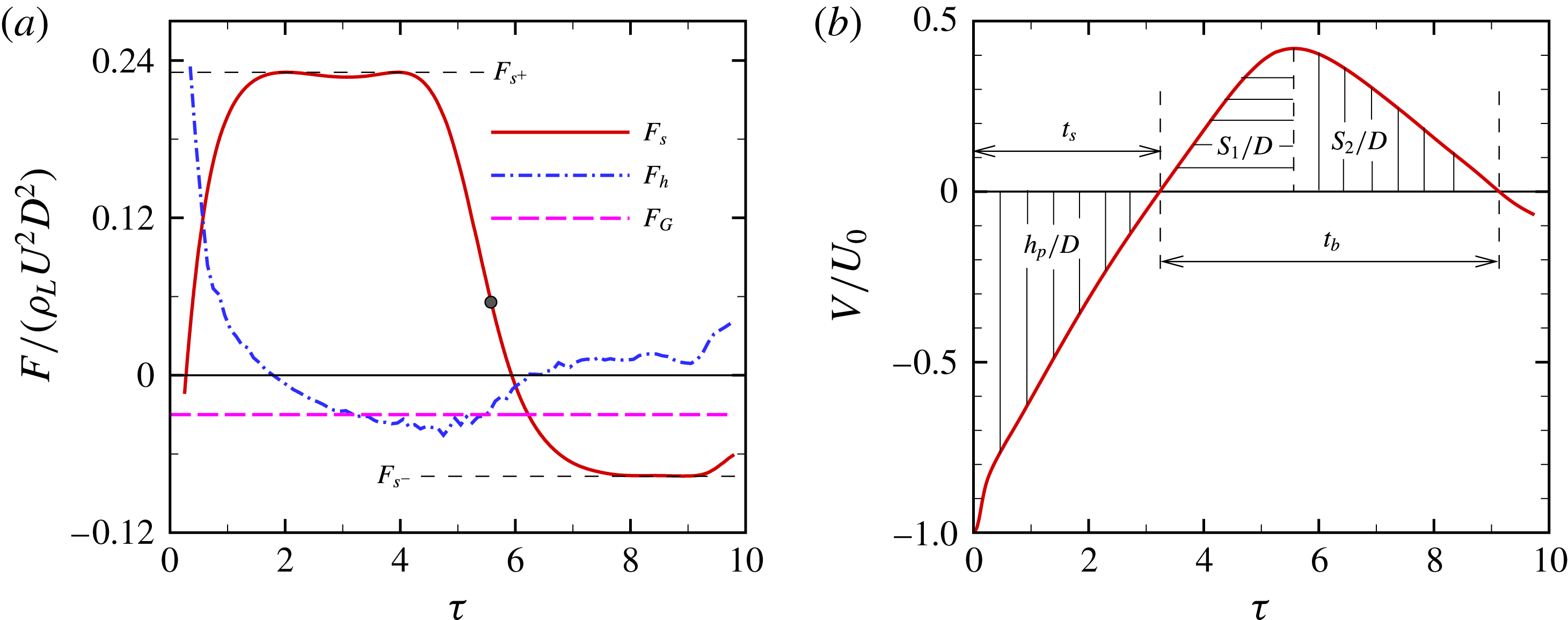
Figure 6 shows the numerical results of an oscillating sphere at
 $We=10.2$
and
 $\unicode[STIX]{x1D703}=120^{\circ }$
, in terms of the vertical component of the forces exerted on and the instantaneous velocity
 $V$
of the sphere. The hydrodynamic force significantly affects
 $V$
at short times after impact (
 $t<0.6$
). After then, the motion of the sphere is mainly dominated by the capillary and gravitational forces. We notice that the value of
 $F_{s}$
is close to either
 $F_{s+}$
(during the period of
 $2<t<5.5$
) or
 $F_{s-}$
(during the period of
 $7<t<10$
). It is due to the fact that the CL tends to stay nearby at
 $\unicode[STIX]{x1D6FD}=\unicode[STIX]{x03C0}-(\unicode[STIX]{x1D703}/2)$
or
 $\unicode[STIX]{x1D6FD}=(\unicode[STIX]{x03C0}-\unicode[STIX]{x1D703})/2$
, more specifically, within a range of
 $\pm 10^{\circ }$
(see figure 3). This also accounts for the observation in figure 6(b) that the sphere velocity experiences two stages of uniform acceleration during the sphere descending and rebounding.
Time variation of the flow quantities for an oscillating sphere at
 $We=10.2$
,
 $Re=1200$
and
 $\unicode[STIX]{x1D703}=120^{\circ }$
: (a) the vertical component of the forces exerted on the sphere and (b) the instantaneous velocity of the sphere. In (a) the forces include the capillary force
 $F_{s}$
, hydrodynamic force
 $F_{h}$
and gravitational force
 $F_{G}$
, and the bullet indicates the moment at which
 $V_{max}$
occurs.

For convenience of analysis, we quantitatively define the duration of sphere descending,
 $t_{s}$
, as the period of time during which the sphere velocity reduces to zero after the initial contact of the sphere with the water surface, and the penetration depth
 $h_{p}$
as the corresponding downward displacement of the sphere (figure 6
b). Similarly, we define the duration of sphere rebounding,
 $t_{b}$
, as the period of time during which the sphere velocity increases to its maximum upward velocity
 $V_{max}$
(accompanied with upward displacement
 $S_{1}$
) and then decreases to zero (accompanied with upward displacement
 $S_{2}$
) (figure 6
b).
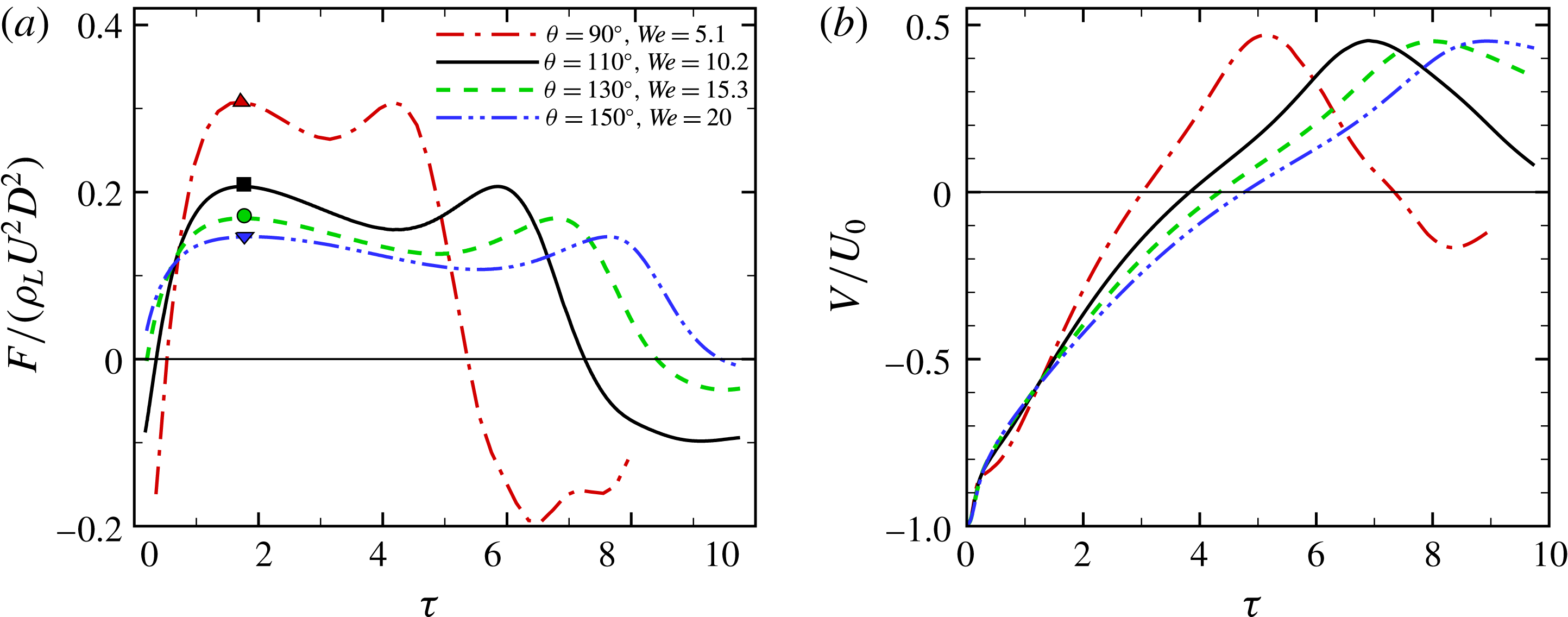
Time variation of the dimensionless
 $F_{s}$
and
 $V$
for the non-sinking spheres near the regime of sphere sinking. In (a), the symbols represent the values of
 $F_{s+}$
at the corresponding contact angle, i.e.
 $90^{\circ }$
(▵),
 $110^{\circ }$
( ◻ ),
 $130^{\circ }$
(◯) and
 $150^{\circ }$
(▿), respectively.

3.3 Flow features at criticality
We investigate here the flow features and the dynamic behaviour of the sphere at the critical conditions for the regime transition to occur. Figure 7 shows the variations of
 $F_{s}$
and
 $V$
for the non-sinking spheres nearly piercing the interface. In these cases, it is clear that
 $F_{s+}$
can be treated as the characteristic value of
 $F_{s}$
during the sphere descending, and accounts for the corresponding roughly uniform deceleration of the sphere. It is also interesting to see that the values of
 $V_{max}$
are more or less the same (
 ${\approx}0.45U_{0}$
) despite the big differences in
 $\unicode[STIX]{x1D703}$
and
 $We$
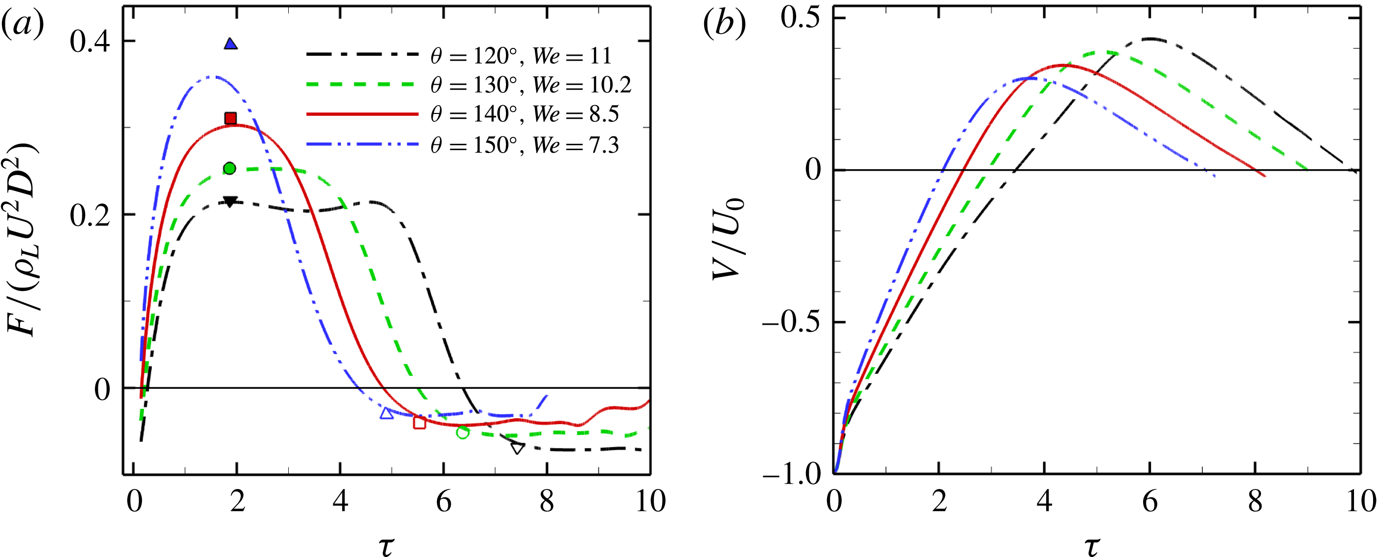
. Figure 8 shows the variations of
 $F_{s}$
and
 $V$
for the oscillating spheres close to the boundary of the bouncing regime. It can be seen that the maximum value of
 $F_{s}$
also reaches
 $F_{s+}$
during the descending of the spheres, except the superhydrophobic one (i.e.
 $\unicode[STIX]{x1D703}=150^{\circ }$
). As a result, two uniform accelerations are also observed during the sphere descending and rebounding for the oscillating spheres at the critical conditions.
Time variation of the dimensionless
 $F_{s}$
and
 $V$
for the oscillating spheres near the regime of sphere bouncing. In (a), the symbols represent the values of
 $F_{s}$
at the corresponding contact angles:
 $120^{\circ }$
(▵),
 $130^{\circ }$
( ◻ ),
 $140^{\circ }$
(◯) and
 $150^{\circ }$
(▿); in particular,
 $F_{s+}$
and
 $F_{s-}$
are represented by the filled and empty symbols, respectively.

The magnitude of the spheres acceleration depends on the combined effect of the capillary force
 $F_{s}$
and gravitational force
 $F_{G}$
. Taking these two forces into account, the two uniform accelerations of the sphere can be simply deduced from Newton’s second law of motion:
 $a_{+}\approx 6\unicode[STIX]{x1D6FE}\sin ^{2}(\unicode[STIX]{x1D703}/2)/(\unicode[STIX]{x1D706}_{\unicode[STIX]{x1D70C}}\unicode[STIX]{x1D70C}_{L}D^{2})-g$
and
 $a_{-}\approx -6\unicode[STIX]{x1D6FE}\cos ^{2}(\unicode[STIX]{x1D703}/2)/(\unicode[STIX]{x1D706}_{\unicode[STIX]{x1D70C}}\unicode[STIX]{x1D70C}_{L}D^{2})-g$
.
It is crucial to determine the duration of sphere descending and rebounding at criticality. Once in contact with the liquid pool, an oscillating sphere is continuously decelerated until it reaches the penetration depth
 $h_{p}$
(figure 6). Obviously, the higher the impact velocity is, the deeper the sphere can reach. However, the sphere cannot lower itself arbitrarily deep into the liquid pool without penetrating the interface. The occurrence of interface penetration relies on the allowable deceleration time before the cavity is sealed by the surface tension and/or gravity. It was suggested that the allowable deceleration time is characterized by
 $t_{c}\sim (\unicode[STIX]{x1D6FE}/(\unicode[STIX]{x1D70C}_{L}g^{3}))^{1/4}=D/U_{0}We^{1/2}Bo^{-3/4}$
, which corresponds to the time for a capillary–gravity wave to travel the capillary length
 $l_{c}\sim \sqrt{\unicode[STIX]{x1D6FE}/(\unicode[STIX]{x1D70C}g)}$
(Vella, Lee & Kim Reference Vella, Lee and Kim2006; Lee & Kim Reference Lee and Kim2008). If the sphere does not sink and reaches the penetration depth, the subsequent rebounding can be considered as a reverse process of the sphere descending, in the sense that the sphere tends to pierce the interface and enter the air. Therefore, it is reasonable to expect that the allowable rebounding time before the contact line detaches from the sphere is also characterized by
 $t_{c}$
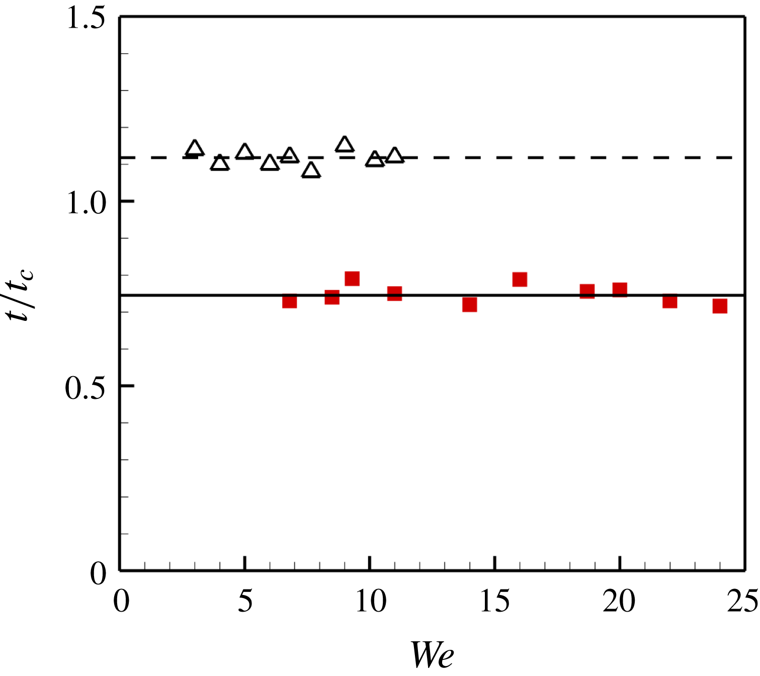
, at the onset of regime transition from oscillating to bouncing. These assumptions of the acceleration duration at criticality are confirmed by the numerical experiments. Figure 9 shows the distribution of
 $t_{s,cr}$
and
 $t_{b,cr}$
as a function of
 $We$
. Here,
 $t_{s,cr}$
represents the descending time of the spheres roughly at the critical conditions of regime transition from non-sinking to sinking, and
 $t_{b,cr}$
represents the rebounding time for the spheres at the critical conditions of regime transition from oscillating to bouncing. It is clear that both
 $t_{s,cr}$
and
 $t_{b,cr}$
strongly correlate with
 $t_{c}$
; more precisely,
 $t_{s,cr}\approx 0.75t_{c}$
and
 $t_{b,cr}\approx 1.1t_{c}$
.
Variation of
 $t_{s,cr}$
( ◼ ) and
 $t_{b,cr}$
(▵) as a function of
 $We$
.

3.4 Criteria for interface penetration
The critical condition for the impact velocity of penetration,
 $U_{p}$
, can be approximately written as
 $U_{p}\sim a_{+}\,t_{c}$
. Because of
 $6\unicode[STIX]{x1D6FE}\sin ^{2}(\unicode[STIX]{x1D703}/2)/(\unicode[STIX]{x1D706}_{\unicode[STIX]{x1D70C}}\unicode[STIX]{x1D70C}_{L}D^{2})\gg g$
, we can neglect the effect of the gravitational force, and consequently obtain
 $$\begin{eqnarray}We_{p}\sim \frac{\sin ^{4}\left({\displaystyle \frac{\unicode[STIX]{x1D703}}{2}}\right)}{\unicode[STIX]{x1D706}_{\unicode[STIX]{x1D70C}}^{2}Bo^{3/2}},\end{eqnarray}$$
where
 $We_{p}=\unicode[STIX]{x1D70C}_{L}U_{p}^{2}D/\unicode[STIX]{x1D6FE}$
. The critical condition suggested by (3.3) is plotted in figures 4 and 5. It is noteworthy that the same proportion factor, i.e.
 $k_{1}=13.9$
, is used. We can see that (3.3) accurately predicts the boundaries between the regions of sinking and non-sinking in both phase diagrams, indicating that the modelling of (3.3) well describes the dependence of
 $We_{p}$
on
 $\unicode[STIX]{x1D703}$
and
 $\unicode[STIX]{x1D706}_{\unicode[STIX]{x1D70C}}$
. For a fixed
 $\unicode[STIX]{x1D703}$
, (3.3) is consistent with the theoretical analysis in Lee & Kim (Reference Lee and Kim2008).
For a non-sinking sphere, one can obtain
 $h_{p}=U_{0}^{2}/(2a_{+})$
. Substituting the expression of
 $a_{+}$
into it, we can get the scaling of
 $h_{p}$
in the dimensionless form as follows
 $$\begin{eqnarray}\frac{h_{p}}{D}\sim \frac{We\,\unicode[STIX]{x1D706}_{\unicode[STIX]{x1D70C}}}{\sin ^{2}\left(\displaystyle \frac{\unicode[STIX]{x1D703}}{2}\right)}.\end{eqnarray}$$
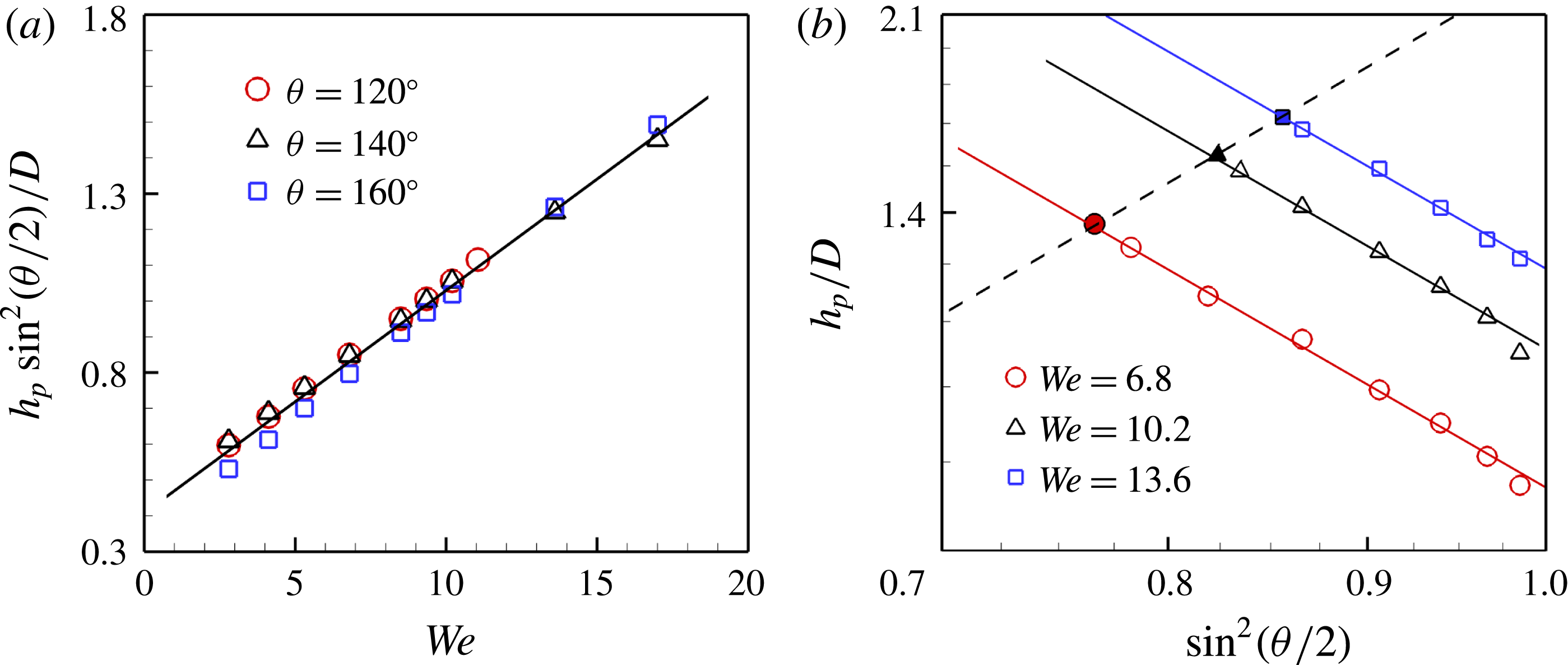
Figure 10(a) shows the numerical results of
 $h_{p}\sin ^{2}(\unicode[STIX]{x1D703}/2)/D$
as a function of
 $We$
at
 $\unicode[STIX]{x1D703}=120^{\circ }$
,
 $140^{\circ }$
and
 $160^{\circ }$
. All the results appear to collapse into a straight line, indicating that the prediction in (3.4) agrees well with the numerical results. Moreover, this suggests that with the same Weber number, the higher the hydrophobicity is, the lower the
 $h_{p}$
is, consistent with the experimental observation (Liu et al.
Reference Liu, Evans and He2016).
If we substitute (3.3) into (3.4), it suggests that the deepest distance that a sphere can dive without penetrating the interface,
 $h_{max}$
, follows
 $$\begin{eqnarray}\frac{h_{max}}{D}\sim \frac{\sin ^{2}\left(\displaystyle \frac{\unicode[STIX]{x1D703}}{2}\right)}{\unicode[STIX]{x1D706}_{\unicode[STIX]{x1D70C}}Bo^{3/2}}.\end{eqnarray}$$
Figure 10(b) shows numerical results of
 $h_{p}/D$
as a function of
 $\sin (\unicode[STIX]{x1D703}/2)$
in a log–log scale, confirming
 $h_{p}/D\propto \sin ^{-2}(\unicode[STIX]{x1D703}/2)$
while
 $h_{max}/D\propto \sin ^{2}(\unicode[STIX]{x1D703}/2)$
.
(a) Variation of rescaled penetration depth
 $h_{p}\sin ^{2}(\unicode[STIX]{x1D703}/2)/D$
as a function of
 $We$
. The solid line represents a linear fitting of the numerical results. (b)
 $h_{p}/D$
as a function of
 $\sin (\unicode[STIX]{x1D703}/2)$
in a log–log scale. The filled symbols denote
 $h_{max}$
at the corresponding
 $We$
. The solid lines denote a slope of
 $-2$
while the dashed line denotes a slope of
 $2$
.

3.5 Criteria for sphere entrapment
It can be assumed that on rebounding the oscillating spheres experience a uniform acceleration (of
 $a_{+}$
) and a subsequent uniform deceleration (of
 $a_{-}$
), in particular near the critical conditions for sphere bouncing (see figure 8
b). The maximum rebounding speed,
 $V_{max}$
, occurs at the moment when the sign of the acceleration changes. Therefore, the duration of the sphere rebounding can be calculated by
 $t_{b}\approx V_{max}(1/a_{+}-1/a_{-})$
, and the dimensionless upward displacements during the two uniform accelerations, i.e.
 $S_{1}$
and
 $S_{2}$
(see figure 6
b), can be calculated by
 $S_{1}=V_{max}^{2}/(2a_{+})$
and
 $S_{2}=-V_{max}^{2}/(2a_{-})$
respectively. We notice that the total displacement in the rebounding process is approximately equal to
 $h_{p}$
(see figure 3
a), i.e.
 $h_{p}\approx S_{1}+S_{2}$
. Consequently, we can obtain
 $$\begin{eqnarray}V_{max}\approx U_{0}\sqrt{\cos ^{2}\displaystyle \left(\frac{\unicode[STIX]{x1D703}}{2}\right)+\frac{1}{6}\unicode[STIX]{x1D706}_{\unicode[STIX]{x1D70C}}Bo}.\end{eqnarray}$$
At the critical conditions for sphere entrapment, we have
 $t_{b,cr}\sim t_{c}$
(see figure 9), or specifically
 $$\begin{eqnarray}V_{max}\left(\frac{1}{a_{+}}-\frac{1}{a_{-}}\right)\sim \left(\frac{\unicode[STIX]{x1D6FE}}{\unicode[STIX]{x1D70C}_{L}g^{3}}\right)^{1/4}.\end{eqnarray}$$
Substituting (3.6) into (3.7) and taking
 $6\sin ^{2}(\unicode[STIX]{x1D703}/2)/(\unicode[STIX]{x1D706}_{\unicode[STIX]{x1D70C}}Bo)\gg 1$
into account, we have the following scaling laws in the dimensionless form for the impact velocity at the onset of sphere bouncing,
 $U_{b}$
,
 $$\begin{eqnarray}We_{b}\sim \frac{1}{\unicode[STIX]{x1D706}_{\unicode[STIX]{x1D70C}}^{2}Bo^{3/2}}\sin ^{4}\left(\frac{\unicode[STIX]{x1D703}}{2}\right)\left(\cos ^{2}\left(\frac{\unicode[STIX]{x1D703}}{2}\right)+\frac{1}{6}\unicode[STIX]{x1D706}_{\unicode[STIX]{x1D70C}}Bo\right),\end{eqnarray}$$
where
 $We_{b}=\unicode[STIX]{x1D70C}_{L}U_{b}^{2}D/\unicode[STIX]{x1D6FE}$
. The theoretical result of (3.8) is plotted in the two phase diagrams in figures 4 and 5, with the same prefactor (
 $k_{2}=31$
). Clearly, (3.8) well represents the boundaries between the bouncing and oscillating spheres obtained by numerical simulations. We note that (3.8) is different from the analysis of Lee & Kim (Reference Lee and Kim2008) for a superhydrophobic sphere (
 $\unicode[STIX]{x1D703}\approx 154^{\circ }$
), i.e.
 $We_{b}\sim Bo^{-3/2}\unicode[STIX]{x1D706}_{\unicode[STIX]{x1D70C}}^{-2}$
. In the late stage of sphere rebounding, the sphere is pulled downwards by the capillary force, the magnitude of which may be of the same order as the the gravitational force, i.e.
 $\cos ^{2}(\unicode[STIX]{x1D703}/2)\sim Bo\unicode[STIX]{x1D706}_{\unicode[STIX]{x1D70C}}/6$
. Therefore, we cannot neglect the gravitational force in the entrapment of the sphere at the interface, especially for superhydrophobic spheres.
4 Conclusion
We numerically investigate the impact of a sphere onto a liquid pool at moderate Reynolds and Weber numbers using the DIIB method, with the aim of gaining an understanding of the role of the wettability in the entrapment of sphere at the liquid–gas interface. The wettability was found to have a significant effect on the magnitude of the capillary force exerted by the interface at the CL, and consequently influences the result of the two important processes after impact: interface penetration and sphere entrapment. Two scaling models have been proposed to interpret the critical conditions of the entrapment of spheres at the interface, and they were shown to be in good agreement with the numerical results. We also found that the penetration depth for a rebounding sphere at certain impact speed followed
 $h_{p}/D\sim \sin ^{-2}(\unicode[STIX]{x1D703}/2)We\unicode[STIX]{x1D706}_{\unicode[STIX]{x1D70C}}$
, while the deepest distance that a sphere can reach without piercing the interface followed
 $h_{max}/D\sim \sin ^{2}(\unicode[STIX]{x1D703}/2)\unicode[STIX]{x1D706}_{\unicode[STIX]{x1D70C}}^{-1}$
. These will be useful for understanding the locomotion of water-jumping insects and designing microrobots walking on water. On the other hand, the proposed dependence on the Bond number remains to be investigated. The contact angle hysteresis is not considered in the present study, but it can be anticipated from the theoretical analysis that the contact angle hysteresis would promote the entrapment of the sphere at the interface.
Acknowledgements
We are grateful for the support of the National Natural Science Foundation of China (grant nos 11425210, 11621202, 11672288), the Strategic Priority Research Program of the Chinese Academy of Sciences (grant no. XDB22040103) and the Fundamental Research Funds for the Central Universities.