

INTRODUCTION
Improving annually resolved reconstructions of past climate is vital for understanding the relative influence of human activity and internal climatic variability as the Earth's climate rapidly responds to increasing greenhouse-gas concentrations. Although continental- to global-scale networks of temperature-sensitive tree-ring records and associated reconstructions continue to be developed (Ahmed et al., Reference Ahmed, Anchukaitis, Asrat, Borgaonkar, Braida, Buckley and Büntgen2013; Wilson et al., Reference Wilson, Anchukaitis, Briffa, Büntgen, Cook, D'Arrigo and Davi2016; Anchukaitis et al., Reference Anchukaitis, Wilson, Briffa, Büntgen, Cook, D'Arrigo and Davi2017; Emile-Geay et al., Reference Emile-Geay, McKay, Kaufman, von Gunten, Wang, Anchukaitis and Abram2017), some regions with high human populations continue to have few known temperature-sensitive tree-ring chronologies that create significant gaps in our understanding of past temperatures. Traditionally, reconstructing past temperatures using tree rings has required sampling at or near altitudinal or latitudinal tree line (Fritts, Reference Fritts1976; Cook and Kairiukstis, Reference Cook and Kairiukstis1990). In several regions, like the northeastern United States, this kind of ecological setting can be rare or nonexistent as tall mountains are not common in these regions.
Previous research has demonstrated that a multispecies dendrochronological approach has the potential to build robust temperature reconstructions in higher-latitude and upper-elevation sites (Frank and Esper, Reference Frank and Esper2005; Garcia-Suarez et al., Reference Garcia-Suarez, Butler and Baillie2009). The use of multiple species in hydroclimate reconstructions in the eastern United States has likewise established that this approach increases both the skill and explained variance of the reconstruction (Maxwell et al., Reference Maxwell, Hessl, Cook and Pederson2011, Reference Maxwell, Harley, Maxwell, Rayback, Pederson, Cook, Barclay, Li and Rayburn2017; Pederson et al., Reference Pederson, Bell, Cook and Lall2013). Although the northeastern United States is temperate and mesic, often receiving more than a meter of precipitation annually (Hayhoe et al., Reference Hayhoe, Wake, Huntington, Luo, Schwartz, Sheffield and Wood2006), many tree populations in the eastern United States have a demonstrated drought limitation (e.g., Hawley et al., Reference Hawley, Wedel and Workman1941; Cook and Jacoby, Reference Cook and Jacoby1977; Stahle et al., Reference Stahle, Cleaveland and Hehr1985; Stahle and Cleaveland, Reference Stahle and Cleaveland1992; Graumlich, Reference Graumlich1993; Pederson et al., Reference Pederson, Bell, Cook and Lall2013, Reference Pederson, D'Amato, Dyer, Foster, Goldblum, Hart and Hessl2015; Maxwell et al., Reference Maxwell, Harley and Robeson2016, Reference Maxwell, Harley, Maxwell, Rayback, Pederson, Cook, Barclay, Li and Rayburn2017). The potential benefit and utility of a multispecies approach, however, has yet to be demonstrated for the reconstruction of temperature in species-rich regions with a paucity of tree-line locations. Thus, although this region is the basis of frequent paleohydroclimatic inquiries (e.g., Cook and Jacoby, Reference Cook and Jacoby1979; Pederson et al., Reference Pederson, Bell, Cook and Lall2013), the perceived lack of classically temperature-limited sites has limited the number of temperature reconstruction efforts.
For the northeastern United States, there have been only two tree-ring-based temperature reconstructions to date. In each case, the records used to reconstruct past temperatures were drawn from a single species. The first was based on Picea rubens Sarg. (red spruce; Conkey, Reference Conkey1986). The most recent reconstruction is based on Chamaecyparis thyoides (L.) B.S.P. (Atlantic white cedar; Pearl et al., Reference Pearl, Anchukaitis, Pederson and Donnelly2017). Although both Picea rubens and Chamaecyparis thyoides have strong temperature responses (Conkey, Reference Conkey1986; Hopton and Pederson, Reference Hopton and Pederson2005; Pearl et al., Reference Pearl, Anchukaitis, Pederson and Donnelly2017), each species has limitations for reconstructing past temperatures. Growth of Picea rubens over the latter portion of the twentieth century, a period key to model validation, has been influenced by atmospheric pollutants (Johnson et al., Reference Johnson, Cook and Siccama1988; Cook and Johnson, Reference Cook and Johnson1989; Mathias and Thomas, Reference Mathias and Thomas2018) and affected the climate response of this species; its growth has recovered in recent decades (Kosiba et al., Reference Kosiba, Schaberg, Rayback and Hawley2017). The high commercial value of Chamaecyparis thyoides as a timber species limits its common maximum age to <150 yr across most of the landscape (Hopton and Pederson, Reference Hopton and Pederson2005; Pearl et al., Reference Pearl, Anchukaitis, Pederson and Donnelly2017). Additionally, Chamaecyparis thyoides loses its positive relation to temperature south of 41°N, restricting reconstructions to the poleward extent of the eastern United States (Pearl et al., Reference Pearl, Anchukaitis, Pederson and Donnelly2017), and is located in more coastal regions (Laderman, Reference Laderman1989), which might inhibit its representativeness of past temperatures in more inland regions. Previous work in the northeastern United States indicates that other species have significant and positive relations to temperature (e.g., Cook and Cole, Reference Cook and Cole1991; Pederson et al., Reference Pederson, Cook, Jacoby, Peteet and Griffin2004; Cook and Pederson, Reference Cook and Pederson2011; Vaganov et al., Reference Vaganov, Anchukaitis, Evans, Hughes, Swetnam and Diaz2011). Supplementing the proven Chamaecyparis thyoides and Picea rubens records with other species having significant and positive relationships with temperature might be beneficial for reconstructing temperatures in the eastern United States and other similar ecoregions.
Here, we test the hypothesis that increasing the tree-ring predictor pools with a greater number of species will improve the skill of paleotemperature reconstructions and allow for the climate history in regions with a limited amount of altitude tree-line environments to be further studied. The northeastern United States was chosen as a testing region because of the availability of tree-ring data from multiple species, its relatively high biodiversity, and a paucity of tree-ring temperature reconstructions in this region. Prior reconstructions in the northeastern United States included winter and spring temperatures (Conkey, Reference Conkey1986; Pearl et al., Reference Pearl, Anchukaitis, Pederson and Donnelly2017). Previous work in the region identified that multiple species have a positive correlation to non-growing-season temperatures (Cook and Cole, Reference Cook and Cole1991; Pederson et al., Reference Pederson, Cook, Jacoby, Peteet and Griffin2004; Hopton and Pederson, Reference Hopton and Pederson2005; Cook and Pederson, Reference Cook and Pederson2011; Martin-Benito and Pederson, Reference Martin-Benito and Pederson2015). Based on this evidence, we focused our investigation on the cool season (January–April) to complement the previous reconstructions based on Picea rubens and Chamaecyparis thyoides. Interestingly, investigations outside of our study region have also indicated that non-growing-season temperatures have a positive influence on long-term tree growth (Duan et al., Reference Duan, Zhang and Lv2013; Pritzkow et al., Reference Pritzkow, Wazny, Heussner, Słowiński, Bieber, Liñán, Helle and Heinrich2016; Balanzategui et al., Reference Balanzategui, Knorr, Heussner, Wazny, Beck, Słowiński and Helle2017; Weigel et al., Reference Weigel, Muffler, Klisz, Kreyling, van der Maaten-Theunissen, Wilmking and Van Der Maaten2018). In sum, these studies suggest that conditions experienced by trees during the dormant season affect the current year's radial increment, though the influence and strength of these dormant season influences has not been thoroughly investigated across multiple species.
We investigate the multispecies hypothesis in two ways: first, we conduct a series of principal component analyses (PCAs) to quantify the variance in cool-season temperature captured by tree-ring chronology networks consisting of an individual temperature-sensitive species (Chamaecyparis thyoides) and also multiple unconventional species; second, we test whether the inclusion of multiple species will supplement the temperature response of Chamaecyparis thyoides, resulting in reconstructions with increased skill, reduced error, and greater explained variance of cool-season temperature records.
METHODS
Study area
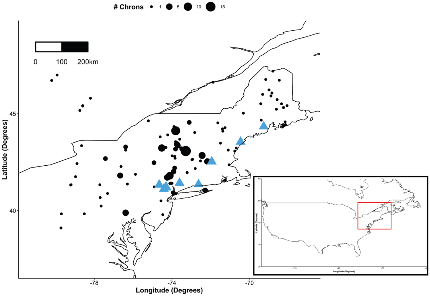
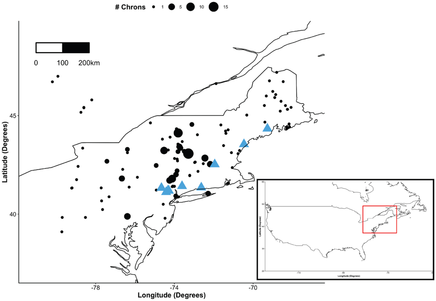
The northeastern United States study region is classified as a mix of hemlock–white pine–northern hardwood forests (Braun, Reference Braun1950; Dyer, Reference Dyer2006), encompassing roughly the area north of Pennsylvania and south of Canada and eastern New York to the coast (37–48°N and 68–82°W; Fig. 1). Recent tree-ring studies have continued to produce new broadleaf and conifer chronologies—from species including Carya glabra (Mill.), pignut hickory; Carya ovata (Mill.) K. Koch, shagbark hickory; Liriodendron tulipifera L., tulip poplar; Quercus montana Willd., chestnut oak; Quercus stellata Wangenh., post oak; Quercus velutina Lam., black oak; and Chamaecyparis thyoides (Hopton and Pederson, Reference Hopton and Pederson2005; Pederson et al., Reference Pederson, Cook, Jacoby, Peteet and Griffin2004, Reference Pederson, Bell, Cook and Lall2013; Martin-Benito and Pederson, Reference Martin-Benito and Pederson2015; Pearl et al., Reference Pearl, Anchukaitis, Pederson and Donnelly2017)—that have expanded the number of species available for study across the region.
Locations of the multispecies network of chronologies used in analysis. Locations of Chamaecyparis thyoides chronologies are highlighted with blue triangles. Size of the point corresponds to the number of chronologies at each location. (For interpretation of the references to color in this figure legend, the reader is referred to the web version of this article.)
Because of the maritime climate along the Atlantic coastline, generally the annual temperature increases from south to north, with coastal temperatures being buffered by proximity to the Atlantic Ocean. During the instrumental period (1895 to 2014), annual mean temperatures range from −6.2°C to 12.0°C, and mean annual precipitation ranges from 21.5 to 239.4 mm. Regional summers are often mild, with summer temperatures ranging from 6.8°C to 31.9°C and summer precipitation ranging from 30.3 to 241.2 mm. Over the instrumental period, summer temperatures in the northeastern United States have increased 1°C (Kunkel et al., Reference Kunkel, Stevens, Stevens, Sun, Janssen, Wuebbles, Rennells, DeGaetano and Dobson2013; Horton et al., Reference Horton, Yohe, Easterling, Kates, Ruth, Sussman, Whelchel, Wolfe, Lipschultz, Melillo, Richmond and Yohe2014). Mean January–April minimum temperatures, the season reconstructed here, can range from −17.2°C to 7.0°C, and precipitation during this season can range from 12.7 to 336.1 mm (PRISM gridded climate product; Daly et al., Reference Daly, Taylor and Gibson1997).
Tree-ring network
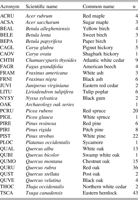
We assembled a diverse network of tree-ring data (Table 1) to assess the effect, if any, that inclusion of multiple species has on the strength and skill of paleotemperature reconstructions. We compiled a database of chronologies available through the International Tree-Ring Data Bank (ITRDB) and multiple collections curated by the authors. This resulted in a total of 228 tree-ring chronologies representing 29 species (Fig. 1). Chronologies consisted of whole ring-width, earlywood, or latewood increments. We included subannual and wood density in these analyses when they were available, as they have been shown to provide differing seasonal response to climate than entire ring widths (Conkey, Reference Conkey1986; Campbell et al., Reference Campbell, McCarroll, Robertson, Loader, Grudd and Gunnarson2011; Griffin et al., Reference Griffin, Woodhouse, Meko, Stahle, Faulstich, Carrillo, Castro and Leavitt2013). Many of these chronologies were not sampled to study climate signals and therefore may not demonstrate the strongest climate-growth relationships for this region. However, we repurposed these diverse records to investigate winter temperature growth response and test our initial hypothesis.
Four-letter acronyms, scientific names, common names, and number of chronologies for species used in the analysis.

Individual ring-width series were standardized with a two-thirds (67%) cubic smoothing spline to reduce the influence of size-related growth trends and other nonclimatic influences such as disturbance (e.g., suppressions because of canopy closure or structural damage and competition release because of gap-phase dynamics; Cook, Reference Cook1985; Cook and Peters, Reference Cook and Peters1997). We also stabilized the variance in each ring-width series through the use of an adaptive power transformation (Cook and Peters, Reference Cook and Peters1997). We used a biweights robust mean to aggregate the individual series to a site-level, species chronology and used the ARSTAN chronology produced by the program ARSTAN (Cook, Reference Cook1985) for all analyses. The ARSTAN chronology retains a portion of the autocorrelation present at the population level and reduces growth anomalies at the individual level with the goal of retaining year-to-year variability driven primarily by climate rather than ecological processes (Cook, Reference Cook1985).
Ring widths of Chamaecyparis thyoides have been shown to be particularly sensitive to cool-season temperature variability (Pederson et al., Reference Pederson, Cook, Jacoby, Peteet and Griffin2004; Hopton and Pederson, Reference Hopton and Pederson2005; Pearl et al., Reference Pearl, Anchukaitis, Pederson and Donnelly2017), and we were interested in identifying additional species in the region that might also be sensitive to the same season to test the hypothesis that increased species diversity improves reconstructions of past temperatures from tree rings. Chamaecyparis thyoides has been used to reconstruct past temperatures in this region (Pearl et al., Reference Pearl, Anchukaitis, Pederson and Donnelly2017), so we use it here as the baseline by which to compare multispecies reconstruction efforts.
All analyses are conducted on the period from 1900 to 1970, the common period of all tree-ring records in our network. Some of the chronologies known to be temperature sensitive, such as Picea rubens from Conkey (Reference Conkey1986; PCRU) and Pinus strobus, were sampled in the 1970s. These temporal limitations omit much of the warming trend of the latter part of the twentieth century (Horton et al., Reference Horton, Yohe, Easterling, Kates, Ruth, Sussman, Whelchel, Wolfe, Lipschultz, Melillo, Richmond and Yohe2014). However, we made this decision to maximize the species included in the network so as to be able to explicitly test the species diversity–paleoreconstruction hypothesis. A finding that these species substantially improve regional temperature reconstructions would provide an impetus to recollect, update, and expand the network of chronologies for these species.
Climate data
We extracted monthly mean precipitation and minimum and maximum temperature from the PRISM gridded (4 km x 4 km resolution) climate product (Daly et al., Reference Daly, Taylor and Gibson1997). For initial climate sensitivity analyses, we extracted site-specific climate data through the use of bilinear interpolation from the raster package in R (Hijmans Reference Hijmans2019). This method is essentially a weighted average for sites that lie adjacent to the grid cell boundaries. Monthly data were aggregated into seasons for correlation analysis based on traditional 3-month seasons as well as regionally significant monthly windows as determined by prior research (Conkey, Reference Conkey1986; Pederson et al., Reference Pederson, Cook, Jacoby, Peteet and Griffin2004; Hopton and Pederson, Reference Hopton and Pederson2005). Seasons included the following: Growing Season = May–August; JanFeb = January and February; JanApr = January through April (hereafter referred to as the “cool” season); Spring = March through May; and Summer = June through August. The gridded PRISM minimum temperature, maximum temperature, and precipitation were used to assess spatial patterns in the climate response. As Chamaecyparis thyoides has been observed to record regional temperature signals (Pearl et al. Reference Pearl, Anchukaitis, Pederson and Donnelly2017), the regional seasonal mean, ranging from 38.0–50.0°N and 80.0–66.5°W, was also calculated and used to calibrate and validate nested reconstruction models of regional minimum JanApr temperature. The Berkeley Earth Surface Temperature data set (BEST; Rohde et al., Reference Rohde, Muller, Jacobsen, Muller, Perlmutter, Rosenfeld, Wurtele, Groom and Wickham2013) minimum temperature data were used as a verification of reconstruction model performance for a similar geographic region as described previously. These data extend back to 1850, whereas the PRISM product extends back to 1895. This longer data set allowed us to compare the PRISM calibrated reconstructed temperatures against a separate observed temperature record that extends beyond the original calibration window.
Temperature response tests
During exploratory analyses, we conducted standard Pearson's correlation analysis on each chronology to determine the strength of the cool-season temperature signal of other species compared with Chamaecyparis thyoides. Cool-season (JanApr) minimum temperature was, again, the variable of interest, but multiple months, including previous year influences, and seasons were analyzed for their respective climate-growth relationships for this species. Climate correlations for all species can be found in Supplementary Figures 1, 2, and 3.
We conducted a series of PCAs (Preisendorfer and Mobley, Reference Preisendorfer and Mobley1988) to quantify the strength and spatial distribution of the regional climate influences on both a Chamaecyparis thyoides–only tree-ring network and a network containing multiple species to identify the strength and spatial distribution of the regional cool-season temperature signal recorded by these networks. Significance of the principal components (PCs) was evaluated using Monte Carlo Rule N simulation tests (Overland and Preisendorfer, Reference Overland and Preisendorfer1982; α = 0.01) with 1000 iterations. We performed a series of Pearson's correlations between the time series (or scores) calculated for each PC and monthly and seasonal minimum temperature, maximum temperatures, and total precipitation. The winter-temperature-influenced mode of variability present in both tree-ring networks was identified using the field correlations with the gridded PRISM temperature data. Trees integrate multiple influences on growth into their annual rings (Cook, Reference Cook1985), and although cool-season temperature may not be the greatest influence on annual growth, prior research with some of the species included in this study shows significant climate-growth relationships with cool-season temperatures (Pederson et al., Reference Pederson, Cook, Jacoby, Peteet and Griffin2004). Therefore, it was reasonable to expect some evidence of cool-season temperature sensitivity in higher-order PCs.
Nested reconstruction
To evaluate the effectiveness of increased species diversity being included in a temperature reconstruction, we reconstructed a regional average JanApr minimum temperature using (1) only Chamaecyparis thyoides chronologies and (2) the 228 chronology multispecies network. The two reconstructions were generated using nested PC regression models (Briffa et al., Reference Briffa, Jones, Wigley, Pilcher and Baillie1986; Cook et al., Reference Cook, Briffa and Jones1994, Reference Cook, Meko, Stahle and Cleaveland1999; Meko, Reference Meko1997). We use the current year and additionally a lag of 1 yr (previous year, t + 1; sensu Frank and Esper, Reference Frank and Esper2005; Maxwell et al., Reference Maxwell, Hessl, Cook and Pederson2011; Pederson et al., Reference Pederson, Bell, Cook and Lall2013) to account for any climate memory of the trees in our reconstruction. In our experience, many of these species in this region have significant lagged relations with prior hydroclimate (Pederson et al., Reference Pederson, Bell, Cook and Lall2013), and given the strong autocorrelation in temperature, we presumed a lagged relationship between growth and temperature in these series, which could be related to the use of stored nonstructural carbon for tree growth (Kagawa et al., Reference Kagawa, Sugimoto and Maximov2006; Carbone et al., Reference Carbone, Czimczik, Keenan, Murakami, Pederson, Schaberg, Xu and Richardson2013; Richardson et al., Reference Richardson, Carbone, Keenan, Czimczik, Hollinger, Murakami, Schaberg and Xu2013). For both models, chronologies (and the lagged t + 1 chronologies) that are significantly (P < 0.05), positively correlated with JanApr minimum temperatures were used as predictors and the January through April regional mean minimum temperature (Tmin) time series as a predictand. This seasonal window was selected because Chamaecyparis thyoides chronologies are correlated strongest with January through April Tmin, and the goal of the article is to attempt to improve on the temperature signal recorded by this species. This allowed us to determine the extent (if any) to which the multispecies network might improve cool-season Tmin reconstructions.
The nested PC regression method takes the common signal of the potential predictors (through a PCA) and regresses the PC against the predictand data (Cook et al., Reference Cook, Meko, Stahle and Cleaveland1999). The nested reconstruction technique sequentially removes the shortest chronologies as potential predictors back through time and generates a new regression model from the remaining chronologies. This method allowed us to include all of the chronologies (despite their length) as potential predictors in the final reconstruction, as all of the chronologies do not need to cover the full period. Additionally, we can extend the reconstruction back further in time beyond the common period (i.e., nest 1), by utilizing the longest chronologies that meet the selection criteria. We use the Akaike information criterion regression model criterion to select the best model (Akaike, Reference Akaike1974; Cook, Reference Cook1987).
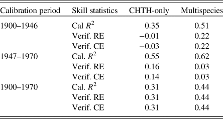
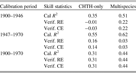
To ensure that the reconstruction accurately captures temperature as shorter chronologies drop out, each nest included in the final reconstruction correlates with the leading nest at r > 0.4. This criterion is relaxed somewhat from Pearl et al. (Reference Pearl, Anchukaitis, Pederson and Donnelly2017), who used a network of Chamaecyparis thyoides chronologies that correlated at r = 0.49. To assess the temporal stability and statistical validity of the reconstruction, we performed split-validation procedures consisting of two-thirds and one-third the length of the common period 1900–1970, alternating the calibration and validation period from 1900 to 1946 and 1947 to 1970. We evaluated reconstruction skill based on the coefficient of determination (R 2), as well as the reduction of error (RE) and coefficient of efficiency (CE) statistics (Table 2). Positive RE and CE statistics indicated skillful reconstructions beyond a naïve prediction using the observed predictand mean (Fritts, Reference Fritts1976; Wigley et al., Reference Wigley, Briffa and Jones1984; Cook et al., Reference Cook, Briffa and Jones1994).
Reconstruction statistics of the first nest for each of the Chamaecyparis thyoides–only (CHTH-Only) and multispecies networks. The calibration R 2 (Cal R 2) and reduction of error and coefficient of efficiency (RE/CE, respectively) statistics for the verification (Verif.) period are shown for each calibration period used in the split calibration/validation procedures (1900–1946 and 1947–1970) and for the full observed period (1900–1970).
We assessed the individual species contribution to explaining the variance in the regional Tmin record by analyzing the absolute value of the standardized regression coefficients, or beta weights of the leading nest (Cook et al., Reference Cook, Meko, Stahle and Cleaveland1999, Reference Cook, D'Arrigo and Mann2002; Maxwell et al., Reference Maxwell, Hessl, Cook and Pederson2011). Absolute values of the beta weights from each predictor chronology used in the first nest that passed the initial screening process (both t0 and t + 1) were summed for each species. This value was then divided by the sum of all the beta weights and then multiplied by 100 to convert into a percentage of contribution of each species. This analysis identifies the species-level contributions to the explained variance (relative explained variance; Frank and Esper, Reference Frank and Esper2005). Results of this are shown as both the cumulative contribution of a species and as individual chronology contributions to the final regression model.
We further verified the relationships found within the multispecies nested reconstruction by comparing the reconstructed temperature record with the BEST data set (Rohde et al., Reference Rohde, Muller, Jacobsen, Muller, Perlmutter, Rosenfeld, Wurtele, Groom and Wickham2013). Correlation analysis between the BEST climate data and the resulting multispecies temperature reconstruction was conducted from 1880 to 1970, the statistically valid period of the reconstruction.
RESULTS
Climatic sensitivity tests and PCA
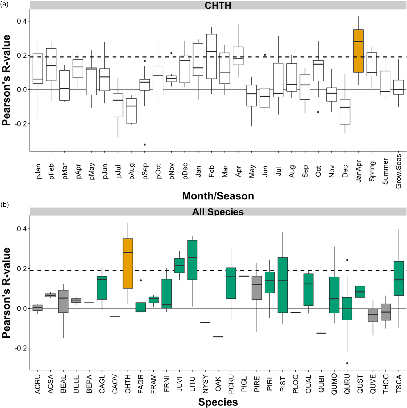
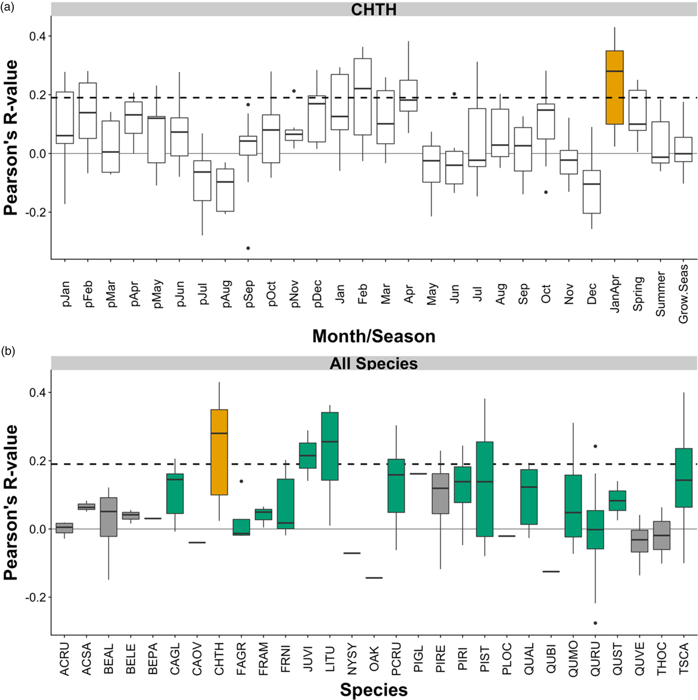
An evaluation of climate-growth relationships in our multispecies network reveals a myriad of climate responses expressed by each species (Supplementary Figs. 1, 2, and 3). Many of the species analyzed show a classic drought response (positive precipitation correlations combined with negative temperature correlations) during the summer months (Supplementary Figs. 1, 2, and 3). However, the winter temperature signals recorded within Chamaecyparis thyoides are the focus of this investigation. Chamaecyparis thyoides shows strong positive relationships with non-growing-season minimum temperature (Fig. 2). Between the months of April and May, there is a sharp decrease in the positive temperature response; therefore, we chose a January to April (JanApr) seasonal window for subsequent analyses. In addition to Chamaecyparis thyoides, multiple species also show moderate sensitivity to non-growing-season climate conditions (Fig. 2; Supplementary Figs. 1, 2, and 3). Of the 29 species analyzed, Chamaecyparis thyoides has the strongest mean correlation with JanApr minimum temperature (0.24±0.14; mean±standard deviation), followed by Liriodendron tulipifera (0.23±0.14) and Juniperus virginiana (0.21±0.10). For both Chamaecyparis thyoides and Liriodendron tulipifera, the JanApr correlations are the strongest climate growth relationship with minimum temperatures throughout the year; however, the monthly April response is the strongest correlation displayed by Juniperus virginiana (0.33±0.09; Supplementary Fig. 1).
Box plots of correlations between Chamaecyparis thyoides (CHTH) tree-ring chronologies and monthly mean minimum temperature (a), and species-level correlations between chronologies and local January–April minimum temperature (b). In panel (a), January–April correlations are highlighted in orange. Climate data are locally extracted PRISM mean minimum temperature. In panel (b), Chamaecyparis thyoides has been highlighted in orange, and additional species that contribute to the multispecies nested reconstruction model are highlighted in green (see Table 1 for definition of four-letter species acronyms). Gray bars represent species that did not contribute to the final multispecies nested reconstruction. The black dashed line represents the one-tailed significance threshold for the period 1900–1970. (For interpretation of the references to color in this figure legend, the reader is referred to the web version of this article.)
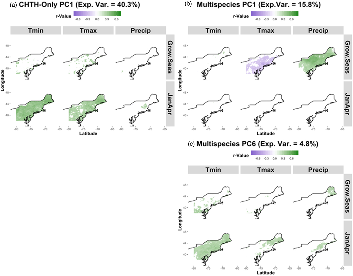
PCA on the nine Chamaecyparis thyoides chronologies resulted in two significant PCs (P < 0.01), the first Chamaecyparis thyoides PC accounting for 40.3% of the variance in that tree-ring network and significantly correlated (r = 0.41) with regional JanApr Tmin for the northeastern United States (Fig. 3a). This pattern, which we identified as the “cool-season temperature PC” appeared when analyzing the multispecies network as well, though as a higher-order PC (PC6). The leading PC from the Chamaecyparis thyoides–only network showed no significant relation to precipitation during the cool season (January–April) or growing season (May–August). This differs from most other species in the region that show strong relationships to drought throughout the growing season (Fig. 3b; Supplementary Figs. 2 and 3). The second PC from the Chamaecyparis thyoides network showed only weak correlations with temperature and precipitation during the growing season.
(color online) Pearson's field correlations with principal component (PC) 1 for Chamaecyparis thyoides (“CHTH-Only”) chronologies (a) and PC1 of the multispecies network (b), and PC6 the “cool-season temperature PC” of the multispecies network (c). Correlations are separated by season (Grow.Seas = May, June, July, August; JanApr = January, February, March, April) and by climate variable (Precip = mean precipitation; Tmax = mean maximum temperature; Tmin = mean minimum temperature). Gridded 4 x 4 km PRISM climate data are used. Only those values meeting significance criteria (α = 0.05) are shown.
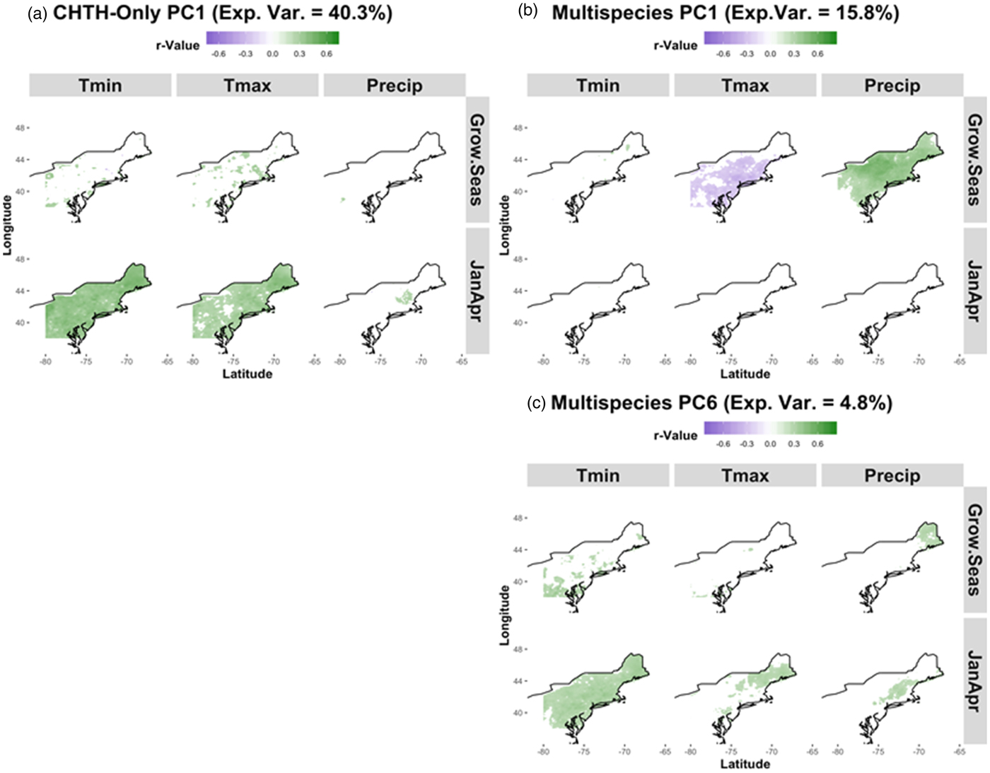
The multispecies network had nine significant PCs. PC1 accounts for almost 16.0% of the variance in the 228-chronology network and showed summer and growing season drought as the dominant signals (Fig. 3b). The cool-season temperature PC for this network, accounting for 4.8% of the variance, was visually identified to reside on PC6 (Fig. 3c), had a significant correlation (r = 0.32) with the regional JanApr Tmin, and revealed a similar strength and spatial pattern of Chamaecyparis thyoides cool-season temperature PC (Fig. 3c). Of note, PC3 of the multispecies network also correlated significantly with JanApr Tmin (r = 0.29), though the strength and spatial extent of the field correlations is reduced compared with PC6 (not shown).
Nested temperature reconstruction
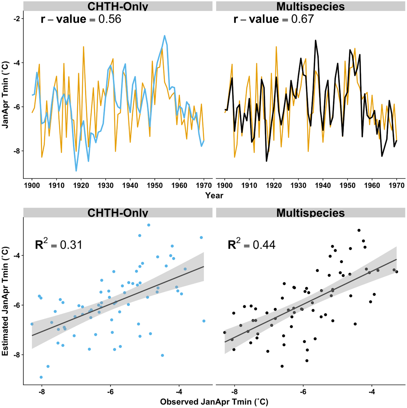
The nested reconstruction calculated from the Chamaecyparis thyoides–only network over the full calibration period showed a significant positive correlation with observed JanApr Tmin (r = 0.56) and explains about 31% of the variance in the Tmin data (Fig. 4). The Chamaecyparis thyoides network temperature reconstruction consisted of 12 out of 18 possible predictors (9 total Chamaecyparis thyoides chronologies with current year [t0] + lagged year [t + 1] time series), indicating that not all of the Chamaecyparis thyoides chronologies were sensitive to cool-season temperature (Fig. 2), consistent with Pearl et al. (Reference Pearl, Anchukaitis, Pederson and Donnelly2017). These 12 predictors, 5 of which consisted of lagged (t + 1) time series, were then used to calculate the reconstruction model. This model did not fully pass the split-sample validation procedures, because negative RE/CE values were observed when using the early calibration period 1900–1946. However, the model did pass calibration/validation tests for the 1947–1970 calibration period, having had positive RE and CE statistics and a calibration R 2 value of 0.56 (Table 2).
Time series and scatter plots for the initial nest of “JanApr” (January, February, March, April; minimum temperature reconstruction models for Chamaecyparis thyoides–only [“CHTH-Only”], light blue) and multispecies chronology networks (“Multispecies,” black) from the northeastern United States for the period 1900 to 1970. A trend line and associated 95% confidence interval is presented for each scatter plot. PRISM data (orange line; observed data) were used to compare model performance as assessed by R 2 and Pearson's r values. (For interpretation of the references to color in this figure legend, the reader is referred to the web version of this article.)
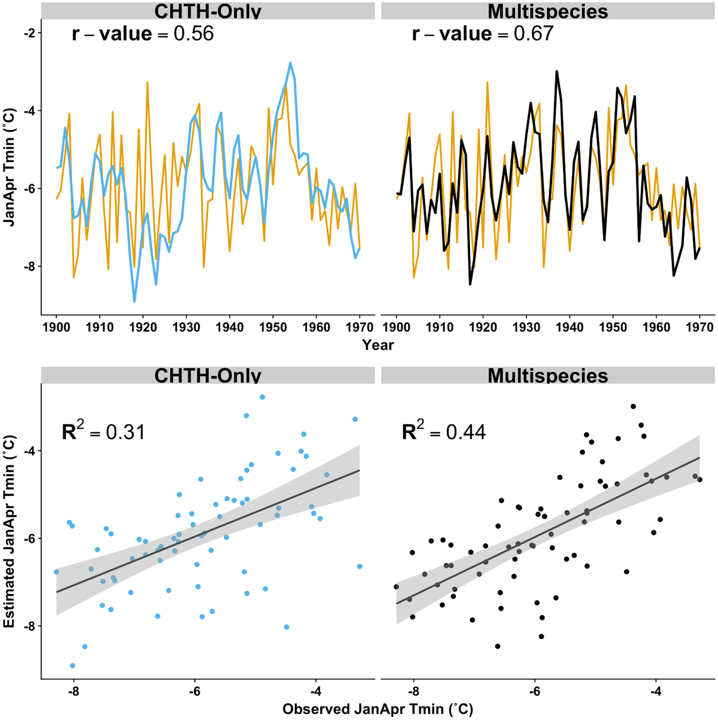
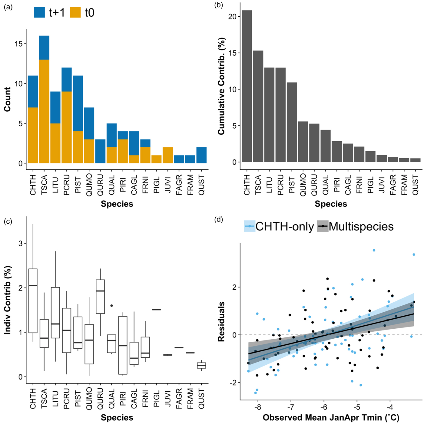
The reconstruction model calculated from the full 228-chronology multispecies network passes split calibration/validation procedures, with an R 2 value of 0.44 (Table 2, Fig. 4) over the 1900–1970 period and a significant positive correlation with observed JanApr Tmin data (r = 0.67; Table 2, Fig. 4). A total of 92 predictors (56% of which were t0 time series; Fig. 4) from 16 species from across the study domain passed the initial screening procedures (Supplementary Fig. 4) and were then used to calculate the leading nest of the reconstruction model. Most predictors were derived from total-ring-width chronologies (90%), with earlywood, latewood, and maximum density chronologies composing 4%, 3%, and 3% of predictors, respectively (Supplementary Fig. 4). Tsuga canadensis contributed the most predictors (13 t0 and 3 t + 1), followed by Chamaecyparis thyoides (7 t0 and 4 t + 1), Picea rubens (9 t0 and 3 t + 1), and Pinus strobus (4 t0 and 7 t + 1; Fig. 5a). Potential predictors available for each species are a function of the number of chronologies in the network (Table 1). Overall, Chamaecyparis thyoides contributed the most to the explained variance in the model (20.8%), followed by Tsuga canadensis (15.3%). The greatest contributing angiosperm species was Liriodendron tulipifera (5 t0 and 4 t + 1), providing 12.9% of the explained variance in the model (Fig. 5b). At the individual chronology level, several angiosperm species contributions are on par with those of Chamaecyparis thyoides (Fig. 5c). Quercus rubra and Carya glabra had median individual chronology contributions of 1.9% and 1.5%, respectively, compared with 2.0% from Chamaecyparis thyoides and 1.2% from Liriodendron tulipifera (Fig. 5c). Additional angiosperm species that contribute to the multispecies reconstruction include Q. stellata, Fraxinus americana, Fraxinus nigra, Fagus grandifolia, and Q. alba
(a) Histogram of predictors that passed selection criteria of each species in the multispecies “JanApr” (January, February, March, April) temperature regression model. Both the current (t0; orange) and the lagged (t + 1; blue) predictors are shown. Four-letter species abbreviations are used and are detailed in Table 1. (b) Cumulative percent contribution derived from multispecies nest 1 regression model beta weights (Pederson et al., Reference Pederson, Bell, Cook and Lall2013) of each species to the minimum temperature regression models. (c) Box plots detailing individual predictor contribution to the multispecies model. (d) Comparison of residuals between estimated and observed JanApr mean temperature between single species (“CHTH-Only,” light blue) and multispecies (black) networks. Trend lines with associated 95% confidence interval are presented for the single species (“CHTH-Only”) and multispecies networks; dashed line indicates ∆ = 0. (For interpretation of the references to color in this figure legend, the reader is referred to the web version of this article.)
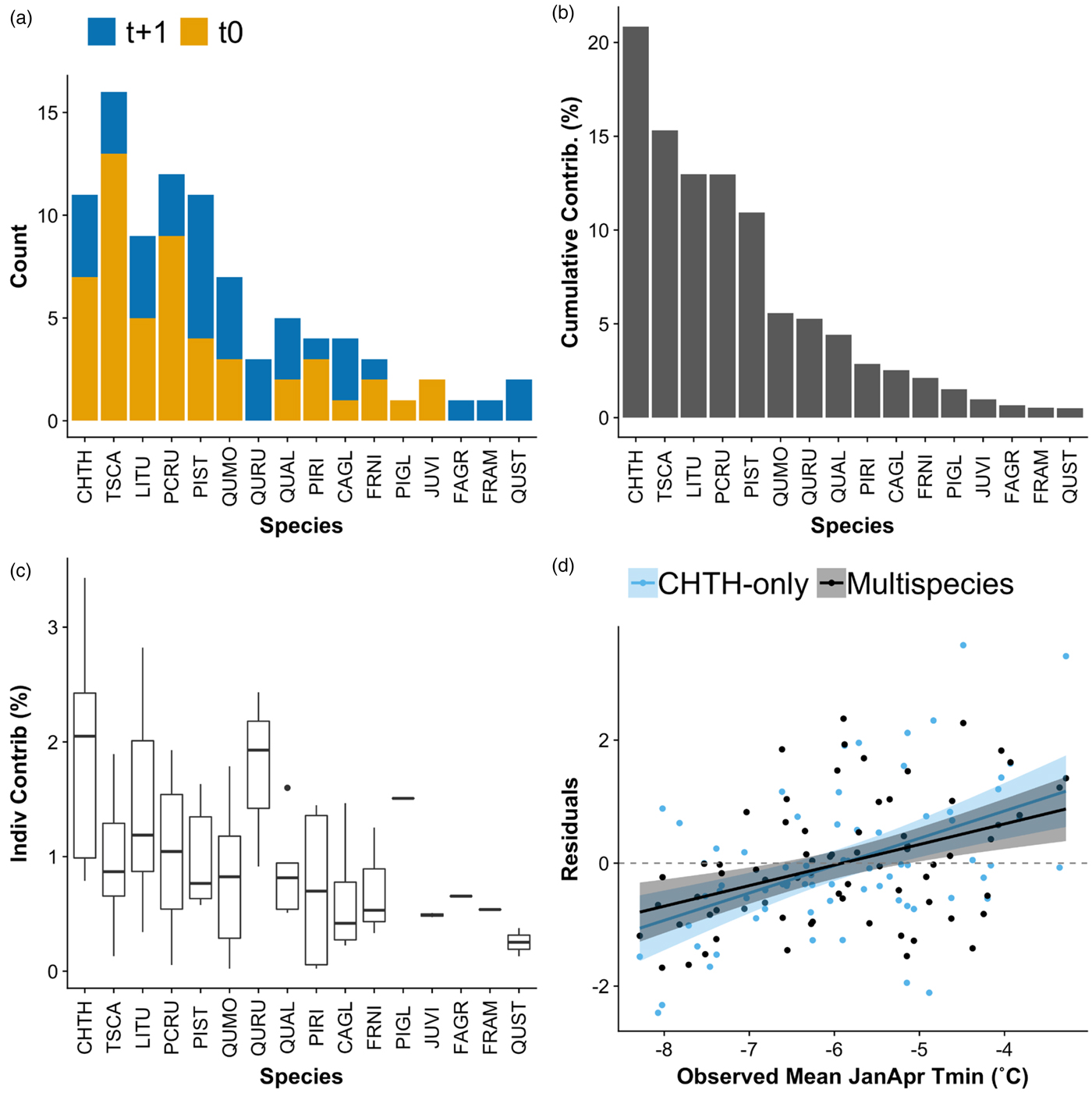
In addition to the increase in explained variance and correlation strength between the multispecies network and the Chamaecyparis thyoides–only network, qualitative improvements in reconstructing both the upper and lower ends of the climate record were observed (Fig. 5d). Although the differences between the residuals of the two models are not significantly different over the entire observed temperature range, at temperatures warmer than −5°C the multispecies model trends toward having lower residual values in a one-way Student's t-test (P = 0.08). Lower residual values indicate a more precise reconstruction of observed temperatures.
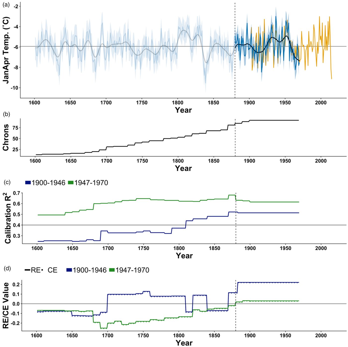
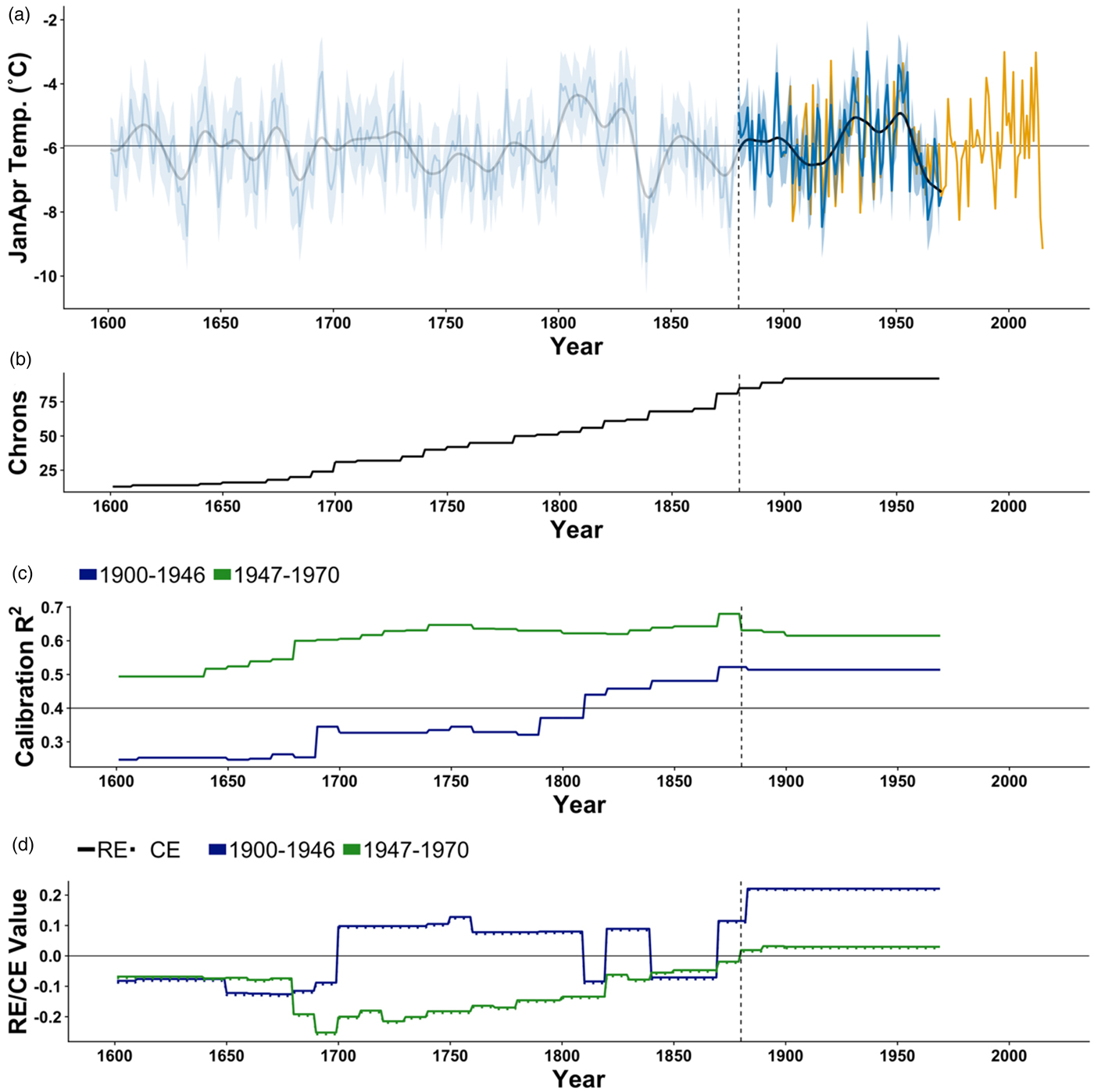
Our split-sample validation procedures revealed that the multispecies model is skillful back to 1880 (Fig. 6). The 1900–1946 calibration period had greater RE/CE statistics (RE = 0.22, CE = 0.22) than the 1947–1970 calibration period (RE = 0.03, CE = 0.03; Table 2, Fig. 5d). The calibration R 2 for nests calculated from the 1947–1970 calibration period are >0.4 throughout the entire length of the reconstruction, whereas the calibration R 2 values of the 1900–1946 calibration period fall below 0.4 at 1810 (Fig. 6c). However, both RE and CE fall below zero at 1879 for the 1947–1970 calibration period (Fig. 6d), indicating the valid period from this tree-ring network exists from 1880 to 1970 (bold region; Fig. 6a). The 1900–1946 period has RE/CE values that are positive until 1869. We compared the multispecies model with the BEST Tmin data as a check on the validity of our reconstruction model. The BEST Tmin record has a strong correlation with the PRISM record for the region (1900–1970; r = 0.91). When compared with the BEST temperature product for the period 1880–1970, the multispecies-network reconstruction has an r value of 0.51.
Multispecies network nested JanApr (January, February, March, April) mean minimum temperature reconstruction (a) and sample depth of chronologies (“Chrons”; b) used from 1600 to 1970. Calibration R 2 values from the split validation protocol of the nested reconstruction (c) and verification coefficient of efficiency and reduction of error statistics (RE/CE; d). Annual reconstructed JanApr temperature values (blue), 20 yr smoothing spline (black), root-mean-square error (ribbon), and observed JanApr PRISM data (orange) are shown in panel (a). The mean reconstructed JanApr minimum temperature (a; horizontal line) is shown to facilitate identification of trend within the data. The reconstruction is skillful (positive RE/CE values), and strong correlations (R 2 > 0.4; gray line; panel c) are observed from 1880 to 1970 (vertical dashed line; bold area). The reconstruction is not considered to be robust before 1880 as RE/CE values turn negative. Split calibration/validation procedures were conducted (d): 1900–1946 (blue) and 1947–1970 (green). (For interpretation of the references to color in this figure legend, the reader is referred to the web version of this article.)
DISCUSSION
A central and early concept in dendrochronology is that trees growing at or near temperature-controlled tree line are favored for reconstructing past temperatures (Fritts, Reference Fritts1976; Cook and Kairiukstis, Reference Cook and Kairiukstis1990). Maintaining such a strict doctrine, however, can omit entire regions that lack altitudinal tree-line environments and could limit our ability to study the full range of climatic variability in regions with large human populations. Here, we have demonstrated that diversifying species within the predictor pool for a temperature reconstruction has the potential to account for a higher proportion of variance, increases the statistical skill of reconstruction models, and better estimates the extreme ranges of observed climate conditions (Table 2, Figs. 4 and 5). Our work supports the findings of prior studies that increased species diversity has the potential to improve tree-ring-based reconstructions, both temperature (e.g., Frank and Esper, Reference Frank and Esper2005; Garcia-Suarez et al., Reference Garcia-Suarez, Butler and Baillie2009) and hydroclimatic (e.g., Maxwell et al., Reference Maxwell, Hessl, Cook and Pederson2011; Pederson et al., Reference Pederson, Bell, Cook and Lall2013). Mounting evidence that some broadleaf deciduous species appear to be sensitive to cool-season conditions (e.g., Pederson et al., Reference Pederson, Cook, Jacoby, Peteet and Griffin2004; Pritzkow et al., Reference Pritzkow, Wazny, Heussner, Słowiński, Bieber, Liñán, Helle and Heinrich2016) will hopefully lead to investigations that improve our understanding of tree physiology and subsequent dynamic vegetation models in botanically rich regions.
Although drought is the dominant climate signal contained in our large and diverse network (Fig. 3b), the cool-season temperature signal persists as a statistically significant component of the network as additional species and chronologies were added to the matrix (P < 0.01; Fig. 3c; Supplementary Fig. 2). Well-documented temperature-sensitive species such as Picea rubens (Conkey, Reference Conkey1986), Tsuga canadensis (Cook and Cole, Reference Cook and Cole1991), and Chamaecyparis thyoides (Hopton and Pederson, Reference Hopton and Pederson2005; Pearl et al., Reference Pearl, Anchukaitis, Pederson and Donnelly2017) contribute greatly to the strength of the nested reconstruction model (Fig. 5b). Broadleaf species underrepresented in the ITRDB (Zhao et al., Reference Zhao, Pederson, D'Orangeville, HilleRisLambers, Boose, Penone, Bauer, Jiang and Manzanedo2018), such as Liriodendron tulipifera, Quercus spp., Fraxinus spp., and Carya glabra, however, also contribute meaningful strength to the regression model (Fig. 5).
Significant relationships with temperatures outside of the growing season seem counterintuitive, but they have been documented for decades (e.g., Brubaker, Reference Brubaker1980). Observations of multiple tree species exhibiting strong positive relationships with cool-season temperatures, however, accumulate with new research (Duan et al., Reference Duan, Zhang and Lv2013; Pritzkow et al., Reference Pritzkow, Wazny, Heussner, Słowiński, Bieber, Liñán, Helle and Heinrich2016; Balanzategui et al., Reference Balanzategui, Knorr, Heussner, Wazny, Beck, Słowiński and Helle2017; Pearl et al., Reference Pearl, Anchukaitis, Pederson and Donnelly2017; Weigel et al., Reference Weigel, Muffler, Klisz, Kreyling, van der Maaten-Theunissen, Wilmking and Van Der Maaten2018). Of the species we investigated, Chamaecyparis thyoides, has the strongest relationship with cool-season temperatures (Fig. 2; Supplementary Fig. 1), allowing for skilled temperature reconstructions (Pearl et al., Reference Pearl, Anchukaitis, Pederson and Donnelly2017) in a region where growing season drought is characteristically studied (Fig. 3; Meko et al., Reference Meko, Cook, Stahle, Stockton and Hughes1993; Cook et al., Reference Cook, Meko, Stahle and Cleaveland1999). Pederson et al. (Reference Pederson, Cook, Jacoby, Peteet and Griffin2004) hypothesized that significant positive cool-season temperature relation to stem growth across multiple species might be because of a reduction of embolism, as experimental research has suggested (Sperry et al., Reference Sperry, Nichols, Sullivan and Eastlack1994; Hacke and Sauter, Reference Hacke and Sauter1996), and fine root mortality in regions lacking a consistent snowpack (Reinmann and Hutyra, Reference Reinmann and Hutyra2016). If the results from these experiments hold true, the signal observed in ring-width variation might result more from a reduction of physical damage and an increase in nonstructural carbohydrates for subsequent growth the following season.
Although the network used in our study was not sampled for cool-season temperature sensitivity, we were able to skillfully reconstruct regional January–April minimum temperature using a multispecies network (Fig. 6). Our reconstruction calculated from Chamaecyparis thyoides did not pass split calibration/validation procedures. This is not altogether unexpected, as Chamaecyparis thyoides has been observed to have weak temperature correlations south of 41°N, and the majority of our Chamaecyparis thyoides chronologies reside in this region (Fig. 1). Although this species has been shown to be a reliable recorder of regional temperature patterns (Hopton and Pederson, Reference Hopton and Pederson2005; Pearl et al., Reference Pearl, Anchukaitis, Pederson and Donnelly2017), it often grows within 200 km of ocean coastlines (Laderman, Reference Laderman1989), leaving much of the western portion of the northeastern United States unrepresented without other species. The improved spatial resolution of our network because of increased species representation (Supplementary Fig. 4) is one explanation for the increase in model skill. However, Pearl et al. (Reference Pearl, Anchukaitis, Pederson and Donnelly2017) showed a rather homogeneous distribution of temperatures across our region, suggesting that greater spatial coverage might not result in greater statistical gain when making reconstructions. A test of spatial representativeness versus species replication with a more homogeneous tree-ring network could give great insight to what is driving the improvement seen with our network.
In addition to expanding the regional representation, incorporating multiple species in climate reconstructions appears to better reconstruct the upper and lower ranges of the climate record (Fig. 5d). Paleoclimate reconstructions calculated from tree rings typically better represent the negative extreme departures from the mean (low precipitation/temperatures) but may not fully capture the positive extremes of the targeted climate variable (Fritts, Reference Fritts1976). For example, trees that are drought sensitive accurately reconstruct the years with low precipitation and often do not accurately depict anomalously wet years in the observed climate record because of trade-offs in the most limiting annual growth influence. This would result in large residual values, especially at the wetter or warmer years of the instrumental record. By including multiple species in our reconstruction, we observed qualitative decreases in the residuals at both the upper and lower extremes of our climate record than the single-species reconstruction, a finding similarly observed in a reconstruction of hydroclimate (Pederson et al., Reference Pederson, Bell, Cook and Lall2013). Although there is not a statistically significant difference between the residuals of the single species and multispecies, the evidence suggests a potential benefit to increasing species diversity in paleoclimate investigations that might increase with expanded sampling efforts.
We are encouraged by our results and see the potential for long temperature reconstructions in regions with little altitudinal tree line such as the northeastern United States, especially as older populations of angiosperm trees are located and sampled. In our analysis, individual contributions of multiple angiosperm species were comparable with those of Chamaecyparis thyoides and Tsuga canadensis, though overall impact of angiosperm species on model performance was ultimately limited by both the number and length of available chronologies (Table 1, Fig. 5). Increasing the sample depth and spatial representation of underrepresented species, such as Liriodendron tulipifera and Carya glabra, and updating the existing tree-ring chronologies to the current date will allow for a longer calibration window that could potentially result in a reconstruction that is valid over a longer time (Babst et al., Reference Babst, Poulter, Bodesheim, Mahecha and Frank2017). The goal of increasing spatial representation in all tree-line-limited regions, realistically, might be a limited one. Although our findings indicate benefits in sampling more species, in some regions there could be substantial limitations simply in the distribution and diversity of species. Temperate forests in our study region are quite species rich compared with other regions such as Europe. Therefore, the benefits gained from including more species in paleotemperature reconstructions may be dependent on available species richness, but also on the willingness for tree-ring scientists to sample understudied species (Zhao et al., Reference Zhao, Pederson, D'Orangeville, HilleRisLambers, Boose, Penone, Bauer, Jiang and Manzanedo2018).
The multispecies reconstruction model is statistically valid back to 1880, where RE/CE values at 1879 fall below zero (Fig. 6c). The decrease in RE/CE values at 1879 (Fig. 6b) appears to be driven by a reduction of younger chronologies through the nesting reconstruction process of contributing species, such as Liriodendron tulipifera and Pinus rigida (Supplementary Table 1). The chronologies that drop out at this time are primarily in eastern New York State. This is a region where Chamaecyparis thyoides has a demonstrably weaker temperature response (Pearl et al. Reference Pearl, Anchukaitis, Pederson and Donnelly2017), indicating that perhaps this region and other parts of southern New England that contain these species should be targeted for further sampling to extend the tree-ring records back further in time. Extending the record of angiosperm species back further into the past requires locating and sampling remnant old-growth forests, as well as the potential inclusion of downed deadwood. However, because the decomposition rates in mesic forests are high, thereby limiting coarse woody debris longevity (Weedon et al., Reference Weedon, Cornwell, Cornelissen, Zanne, Wirth and Coomes2009; Alexander et al., Reference Alexander, Rollinson, Moore, Speer and Rubino2018), the inclusion of archaeological material is critical to this effort (see Stahle, Reference Stahle1979; Cook and Callahan, Reference Cook and Callahan1992; Baas and Rubino, Reference Baas and Rubino2014; de Graauw, Reference de Graauw2017).
The contribution of Liriodendron tulipifera to temperature reconstructions has been, until now, unexplored. This species has also been traditionally underrepresented in both hydroclimatic reconstructions and the ITRDB (Maxwell et al., Reference Maxwell, Hessl, Cook and Pederson2011, Reference Maxwell, Harley, Maxwell, Rayback, Pederson, Cook, Barclay, Li and Rayburn2017; Pederson et al., Reference Pederson, Bell, Cook and Lall2013; Zhao et al., Reference Zhao, Pederson, D'Orangeville, HilleRisLambers, Boose, Penone, Bauer, Jiang and Manzanedo2018). Investigations within the last decade have shown Liriodendron tulipifera to be highly sensitive to climatic variation (Maxwell et al., Reference Maxwell, Hessl, Cook and Pederson2011, Reference Maxwell, Harley, Maxwell, Rayback, Pederson, Cook, Barclay, Li and Rayburn2015; Martin-Benito and Pederson, Reference Martin-Benito and Pederson2015; Lévesque et al., Reference Lévesque, Andreu-Hayles and Pederson2017). Here we find significant potential to increase model strength in the reconstruction of past cold-season temperatures toward the poleward end of its range (Fig. 1; Supplementary Table 1; Prasad et al., Reference Prasad, Iverson, Peters and Matthews2014). In an analysis of the Liriodendron tulipifera’s climatic sensitivity over much of its range, Martin-Benito and Pederson (Reference Martin-Benito and Pederson2015) found that the cool-season temperature sensitivity of Liriodendron tulipifera is strongest along the spine of the Appalachian Mountains in the more equatorial portion of its distribution. These findings further support the idea that more species in temperate mesic forests warrant renewed investigation for the longevity and potential use in tree-ring based reconstructions of past climate (Maxwell, Reference Maxwell2016). Such work will be especially important as climate science attempts to refine the range of historical climate conditions in temperate regions around the world.
CONCLUSIONS
In a region where finding a clear temperature signal is difficult because of the absence of altitudinal or latitudinal tree-line environments, we find that the inclusion of greater species diversity in the predictor pool has the potential to reconstruct past temperatures with greater statistical strength than with single species selected a priori for their temperature sensitivity. We encourage future research efforts that target broadleaf species in different parts of the eastern United States and in other temperate mesic regions with great species diversity, such as East Asia. This recommendation is supported by the stronger than expected climate responses observed in broadleaf species that typify the underrepresentation of this class of trees in the ITRDB (Zhao et al., Reference Zhao, Pederson, D'Orangeville, HilleRisLambers, Boose, Penone, Bauer, Jiang and Manzanedo2018). Continuing to study more species will likely broaden our perspective on how individual trees, species, and forests at less extreme sites interact with their environment (Carrer, Reference Carrer2011; Pederson et al., Reference Pederson, Tackett, McEwan, Clark, Cooper, Brosi, Eaton and Stockwell2012; Cavin and Jump, Reference Cavin and Jump2016), ultimately improving our understanding of past climate conditions in currently underrepresented regions.
ACKNOWLEDGMENTS
This work was supported by grants from the U.S. National Science Foundation (NSF) Paleo Perspectives on Climate Change program (P2C2; AGS-1304262) and NSF Macrosystems Biology (EF-1241930; the PalEON Project, paleonproject.org).
SUPPLEMENTARY MATERIAL
The supplementary material for this article can be found at https://doi.org/10.1017/qua.2019.33