1 Introduction
Steady incoming flow past a long smooth circular cylinder at low Reynolds numbers is one of the most classical fluid mechanics problems. In this case, the flow is governed by the Reynolds number
 $Re$
(
 $=UD/\unicode[STIX]{x1D708}$
) only, where
 $U$
is the incoming flow velocity,
 $D$
is the cylinder diameter and
 $\unicode[STIX]{x1D708}$
is the kinematic viscosity of the fluid. It is well known that for flow past a circular cylinder vortex shedding emerges at
 $Re=47$
(e.g. Henderson Reference Henderson1997). The vortex shedding frequency
 $f$
is commonly presented in a dimensionless form, namely the Strouhal number
 $St$
(
 $=\,f\,D/U$
).
The variation of
 $St$
with
 $Re$
has been studied extensively, owing to its fundamental as well as practical significance. For example, Norberg (Reference Norberg1994) and Fey, König & Eckelmann (Reference Fey, König and Eckelmann1998) both reported the
 $St{-}Re$
relationship for
 $Re$
from the onset of vortex shedding (
 $Re=47$
) to the point just before boundary layer transition (
 $Re\sim 2\times 10^{5}$
). Fey et al. (Reference Fey, König and Eckelmann1998) also categorized the
 $St{-}Re$
curve into different regimes based on different flow instabilities, such as the secondary wake instability at
 $Re\sim 180$
and the shear layer instability at
 $Re\sim 1300$
. In addition, Schewe (Reference Schewe1983) reported the
 $St{-}Re$
relationship for
 $Re$
from
 $2\times 10^{4}$
to
 $7\times 10^{6}$
, covering the range of boundary layer transition to turbulence.
A number of empirical and semi-empirical formulae for the
 $St{-}Re$
relationship over certain ranges of
 $Re$
were proposed, for example:
-
(1)
 $St=A+B/Re$
by Roshko (Reference Roshko1954) and Ponta & Aref (Reference Ponta and Aref2004),
-
(2)
$St=A+B/Re^{1/2}$
by Fey et al. (Reference Fey, König and Eckelmann1998), Williamson & Brown (Reference Williamson and Brown1998) and Ponta (Reference Ponta2006), and -
(3)
$St=1/(A+B/Re)$
by Roushan & Wu (Reference Roushan and Wu2005),



where
 $A$
and
 $B$
are curve-fitting coefficients. Although some semi-empirical formulae were established by taking into account physical properties related to vortex shedding, such as the variation of the shear layer thickness with
 $Re^{-1/2}$
(Williamson & Brown Reference Williamson and Brown1998), the transport of vorticity (Ponta & Aref Reference Ponta and Aref2004), or the vortex street structure (Roushan & Wu Reference Roushan and Wu2005), the formulae were still derived ultimately through curve fitting of the actual
 $St{-}Re$
relationship.
In the low
 $Re$
range, Williamson (Reference Williamson1996a
) studied the
 $St{-}Re$
relationship in the wake transition regime, and found two discontinuities in the
 $St{-}Re$
curve:
-
(1) a sudden drop of
$St$
at the onset of the secondary wake instability of
$Re\sim 180$
, where the fully developed wake flow structure becomes mode A with large-scale vortex dislocations; -
(2) a twin-peaked regime of
$Re=230{-}260$
where a gradual wake transition from mode A with dislocations to mode B takes place.


Williamson (Reference Williamson1996a
) suggested that the sudden drop of
 $St$
at
 $Re\sim 180$
is due to the occurrence of vortex dislocations. In contrast, Henderson (Reference Henderson1997) suggested that it is due to the mode A instability only, irrespective of the dislocations. Henderson’s (Reference Henderson1997) argument was supported by the three-dimensional (3D) direct numerical simulation (DNS) of a case at
 $Re=195$
with a restricted spanwise domain length of
 $3.96D$
. By restricting the spanwise domain length to approximately the most unstable wavelength of mode A, the fully developed wake structure is represented by one pair of ordered mode A structures, while vortex dislocation is suppressed. Nevertheless, as the 3D wake structure develops, the Strouhal number drops from its counterpart calculated by two-dimensional (2D) DNS. However, the fundamental cause for the variation of
 $St$
with the development of different 3D wake structures was not revealed.
Roshko (Reference Roshko1955) suggested that the vortex shedding frequency in the wake of a bluff body would scale better on the velocity at separation (
 $U_{s}$
) and the wake width (
 $D^{\prime }$
), rather than simply on
 $U$
and
 $D$
. The Strouhal number based on such a definition was called the wake Strouhal number
 $St^{\ast }$
(
 $=\,f\,D^{\prime }/U_{s}$
) in Roshko (Reference Roshko1955). Based on experimental measurements on three bluff-body shapes, including a flat plate, a
 $90^{\circ }$
wedge and a circular cylinder, Roshko (Reference Roshko1955) obtained a relatively universal
 $St^{\ast }$
of approximately 0.16 (
 $\pm 0.01$
) for the three bodies for the wake Reynolds number
 $Re^{\ast }$
(
 $=U_{s}D^{\prime }/\unicode[STIX]{x1D708}$
) in the range of approximately
 $1\times 10^{4}$
to
 $4.4\times 10^{4}$
. However, relatively large and irregular discrepancies of
 $St^{\ast }$
ranged between 0.16 and 0.20 were observed for
 $Re^{\ast }$
below approximately
 $1\times 10^{4}$
.
By studying the experimental
 $St^{\ast }{-}Re$
data for a circular cylinder, Williamson & Brown (Reference Williamson and Brown1998) found a relatively universal
 $St^{\ast }$
of approximately 0.176 (with variations between 0.164 and 0.186) for
 $Re$
in the range of 55 to
 $1.4\times 10^{5}$
. Compared with the results reported in Roshko (Reference Roshko1955), the more uniform
 $St^{\ast }$
values in the low
 $Re$
range in Williamson & Brown (Reference Williamson and Brown1998) may be attributed to an improvement in the quality of the experimental data, for example through elimination of the ‘end effect’ of the cylinder (Williamson Reference Williamson1996a
).
In light of the previous works, the present study aims at examining the
 $St^{\ast }{-}Re$
relationship in the low
 $Re$
range of
 $Re\leqslant 1000$
by using both 2D and 3D DNS. For the rest of the paper, subscripts ‘2D’ and ‘3D’ are used to distinguish the Strouhal numbers calculated with 2D and 3D DNS, respectively. An advantage of using DNS is that high-resolution flow properties, such as
 $U_{s}$
and
 $D^{\prime }$
, are available to allow for a better estimation and a thorough analysis of the 2D and 3D
 $St^{\ast }{-}Re$
relationships. The physical mechanism for the variation of
 $St$
with the development of different 3D wake structures is also investigated.
2 Numerical model
2.1 Numerical method
The present DNS are carried out with OpenFOAM (www.openfoam.org) to solve the continuity and incompressible Navier–Stokes equations:
 $$\begin{eqnarray}\displaystyle & \displaystyle \frac{\unicode[STIX]{x2202}u_{i}}{\unicode[STIX]{x2202}x_{i}}=0, & \displaystyle\end{eqnarray}$$
 $$\begin{eqnarray}\displaystyle & \displaystyle \frac{\unicode[STIX]{x2202}u_{i}}{\unicode[STIX]{x2202}t}+u_{j}\frac{\unicode[STIX]{x2202}u_{i}}{\unicode[STIX]{x2202}x_{j}}=-\frac{1}{\unicode[STIX]{x1D70C}}\frac{\unicode[STIX]{x2202}p}{\unicode[STIX]{x2202}x_{i}}+\unicode[STIX]{x1D708}\frac{\unicode[STIX]{x2202}^{2}u_{i}}{\unicode[STIX]{x2202}x_{j}\unicode[STIX]{x2202}x_{j}}, & \displaystyle\end{eqnarray}$$
where
 $(x_{1},x_{2},x_{3})=(x,y,z)$
are Cartesian coordinates,
 $u_{i}$
is the velocity component in the direction
 $x_{i}$
,
 $t$
is time,
 $\unicode[STIX]{x1D70C}$
is fluid density and
 $p$
is pressure. The same numerical approach as used in Jiang et al. (Reference Jiang, Cheng, Draper, An and Tong2016, Reference Jiang, Cheng, Draper and An2017a
,Reference Jiang, Cheng, Draper and An
b
) is adopted here. Specifically, the finite-volume method (FVM) and the pressure-implicit with splitting of operators (PISO) algorithm (Issa Reference Issa1986) are used to solve the equations.
2.2 Computational domain and mesh
In the present study, DNS are carried out for
 $Re$
up to 1000. For
 $Re\leqslant 300$
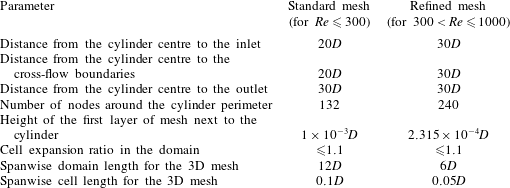
, the standard 2D and 3D meshes used in Jiang et al. (Reference Jiang, Cheng, Draper, An and Tong2016) are adopted. For
 $300<Re\leqslant 1000$
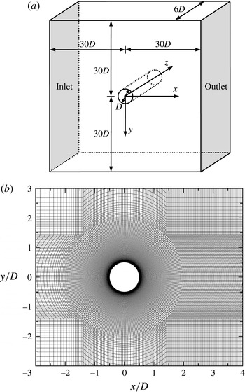
, a refined mesh over that used in Jiang et al. (Reference Jiang, Cheng, Draper, An and Tong2016) is used. Some key parameters for the standard and refined meshes are listed in table 1. Figure 1 shows a schematic model and a close-up view of the refined mesh. A relatively high mesh resolution is used in the near wake by specifying a streamwise mesh size varying linearly from
 $0.0375D$
at
 $x/D=2$
to
 $0.1D$
at
 $x/D=10$
.
The refined mesh used for
 $300<Re\leqslant 1000$
: (a) schematic model of the computational domain, and (b) close-up view of the mesh near the cylinder.

Parameters for the standard and refined meshes used in this study.

A mesh convergence check of the refined 2D and 3D meshes is reported in appendix A. In particular, a reduction in the spanwise domain length from
 $12D$
to
 $6D$
is justified, given that the relatively large-scale mode A structure (with a spanwise wavelength of
 ${\sim}4D$
) disappears at
 $Re\sim 270$
and the small-scale mode B structure (with a spanwise wavelength of
 ${<}1D$
) becomes the only wake flow mode for
 $Re>270$
. In addition, the spanwise cell length is reduced from
 $0.1D$
to
 $0.05D$
, since the mode B structure becomes finer with further increase in
 $Re$
.
3 Determination of
$St_{2D}^{\ast }$

3.1 Previous method
The wake Strouhal number
 $St^{\ast }$
, as proposed by Roshko (Reference Roshko1955), is calculated in the present study by
 $$\begin{eqnarray}St^{\ast }=\,f_{L}D^{\prime }/U_{s}=St\frac{U}{U_{s}}\frac{D^{\prime }}{D},\end{eqnarray}$$
where
 $f_{L}$
is the frequency of the fluctuating lift force. It was shown in Roshko (Reference Roshko1955) and Williamson & Brown (Reference Williamson and Brown1998) that
 $St^{\ast }$
would be nearly constant over a wide range of
 $Re$
. In both studies,
 $U_{s}$
was calculated by
 $$\begin{eqnarray}\frac{U_{s}}{U}=\sqrt{1-C_{pb}},\end{eqnarray}$$
where
 $C_{pb}$
is the base pressure coefficient defined in (A 5), which is a negative value. The wake width
 $D^{\prime }$
calculated in Williamson & Brown (Reference Williamson and Brown1998) was defined as
 $$\begin{eqnarray}\frac{D^{\prime }}{D}=1+\frac{2\unicode[STIX]{x1D6FF}}{D},\end{eqnarray}$$
where
 $\unicode[STIX]{x1D6FF}$
is the separated shear layer thickness evaluated based on the time-averaged streamwise velocity profile sampled at the streamwise location of
 $x/D=1$
(refer to Williamson & Brown (Reference Williamson and Brown1998) for details).
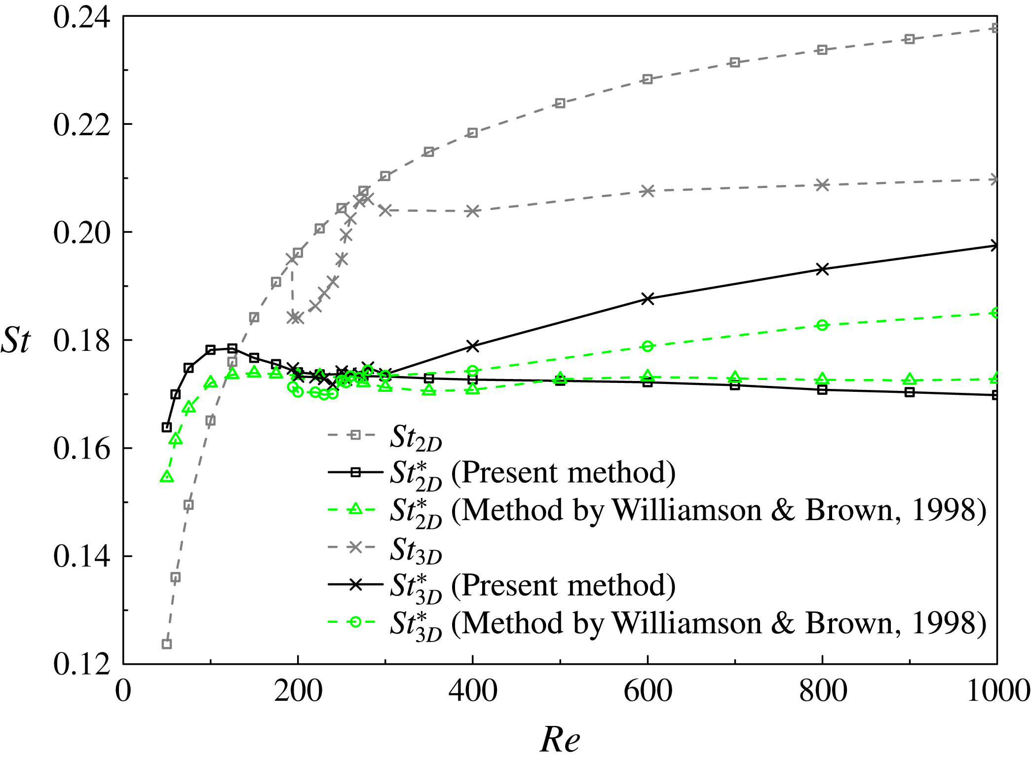
As shown in figure 2, by adopting the method of Williamson & Brown (Reference Williamson and Brown1998), the
 $St_{2D}^{\ast }$
values for
 $Re$
in the extended laminar regime up to
 $Re=1000$
are indeed more uniform than the original
 $St_{2D}$
values. However, based on the
 $C_{pb}$
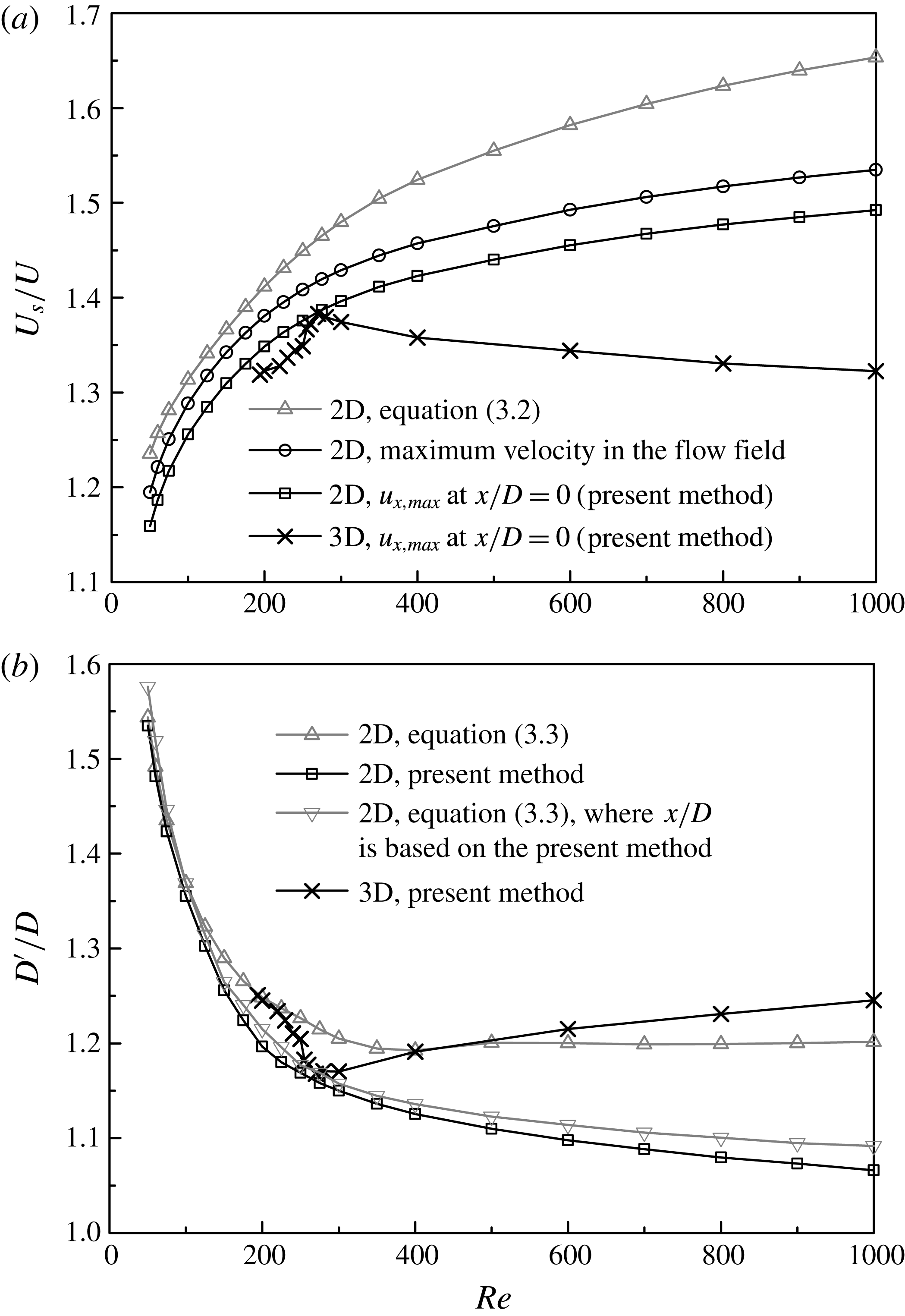
values calculated in the present DNS, it is found that (3.2) overpredicts
 $U_{s}$
for
 $Re$
larger than approximately 200, as the predicted
 $U_{s}$
becomes increasingly larger than the maximum velocity of the whole flow field (figure 3
a). In addition, the wake width calculated by (3.3) (figure 3
b) is based on the streamwise velocity profile measured at a fixed streamwise location of
 $x/D=1$
, whereas for 2D flows the streamwise length of the recirculation region reduces monotonically with increasing
 $Re$
and the vortices may roll up well before
 $x/D=1$
(see figure 7
a for an example at
 $Re=1000$
), such that the wake width measured at
 $x/D=1$
may not represent the actual wake width that initiates the vortex rolling up and shedding. Nevertheless, for
 $Re$
larger than approximately 200, the overpredictions of both
 $U_{s}$
and
 $D^{\prime }$
by using (3.2) and (3.3) do not necessarily lead to an inaccurate prediction of
 $St_{2D}^{\ast }$
, since the overpredictions of
 $U_{s}$
and
 $D^{\prime }$
are incidentally at a similar level and thus cancel out in (3.1).
The 2D and 3D
 $St{-}Re$
relationships for flow past a circular cylinder.

The (a)
 $U_{s}{-}Re$
and (b)
 $D^{\prime }{-}Re$
relationships, evaluated based on different methods.

3.2 An improved method
In the present study, an improved method is proposed for the determination of
 $U_{s}$
and
 $D^{\prime }$
. It is important to note that the
 $U_{s}$
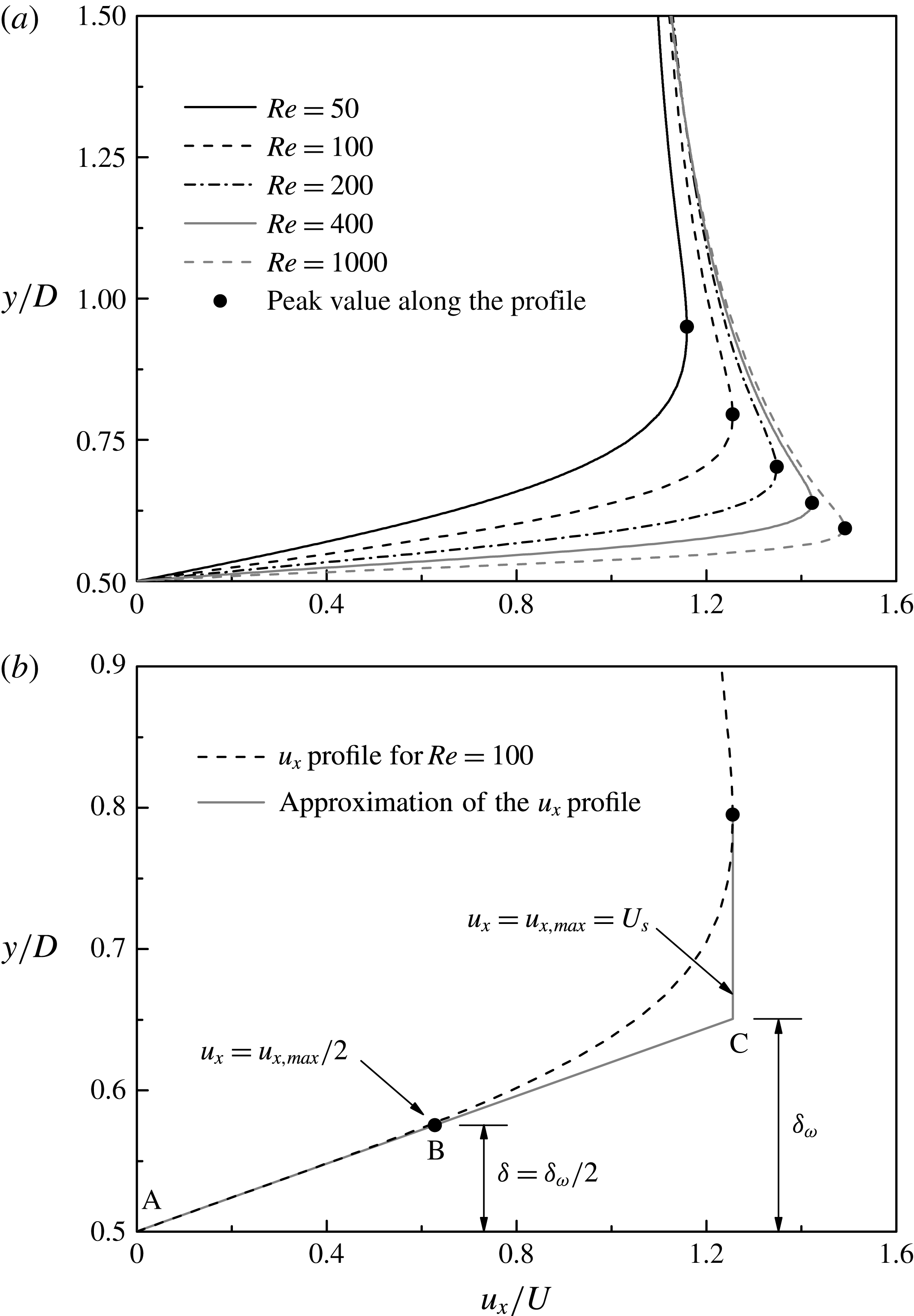
value should be considered as a velocity representative of the regional flow field near the separation, rather than the velocity at a particular point. This is because the velocity profile still develops as the flow travels from the separation point to the point where vortices start to roll up, and the vortex shedding frequency is affected by the velocity at the latter point. In this study,
 $U_{s}$
is chosen as the peak value (
 $u_{x,max}$
) along the time-averaged streamwise velocity (
 $u_{x}$
) profile at
 $x/D=0$
, as denoted by a solid dot in figure 4(a). The reason for the choice of
 $U_{s}$
is illustrated in figure 4(b) with the
 $u_{x}$
profile for
 $Re=100$
as an example. In figure 4(b), the shear layer vorticity thickness
 $\unicode[STIX]{x1D6FF}_{\unicode[STIX]{x1D714}}$
is calculated as (Monkewitz Reference Monkewitz1988):
 $$\begin{eqnarray}\unicode[STIX]{x1D6FF}_{\unicode[STIX]{x1D714}}=\frac{u_{x,max}}{|\text{d}u_{x}/\text{d}y|_{max}}.\end{eqnarray}$$
The separated shear layer thickness
 $\unicode[STIX]{x1D6FF}$
is calculated as
 $\unicode[STIX]{x1D6FF}=\unicode[STIX]{x1D6FF}_{\unicode[STIX]{x1D714}}/2$
(Williamson & Brown Reference Williamson and Brown1998), and the streamwise velocity at point B, namely the midpoint of line AC, is
 $u_{x,max}/2$
. As shown in figure 4(b), line AB serves as a good approximation of the
 $u_{x}$
profile along the separating shear layer, and therefore
 $u_{x,max}/4$
is considered to be a good approximation of the mean streamwise velocity within the shear layer. In the present study,
 $U_{s}$
is chosen as
 $u_{x,max}$
rather than as
 $u_{x,max}/2$
or
 $u_{x,max}/4$
so as to facilitate comparison with the results of Williamson & Brown (Reference Williamson and Brown1998). The
 $U_{s}{-}Re$
relationship based on the present method is plotted in figure 3(a).
Time-averaged streamwise velocity profiles sampled at
 $x/D=0$
: (a) for various
 $Re$
values, and (b) for
 $Re=100$
.

On the other hand, the
 $D^{\prime }$
value in the present study is determined directly based on the spanwise vorticity contours of the time-averaged flow field. The spanwise vorticity
 $\unicode[STIX]{x1D714}_{z}$
is defined in a non-dimensional form as
 $$\begin{eqnarray}\unicode[STIX]{x1D714}_{z}=\left(\frac{\unicode[STIX]{x2202}u_{y}}{\unicode[STIX]{x2202}x}-\frac{\unicode[STIX]{x2202}u_{x}}{\unicode[STIX]{x2202}y}\right)\frac{D}{U}.\end{eqnarray}$$
As illustrated in figure 5,
 $D^{\prime }$
is chosen as the largest vertical distance between the positive and negative
 $\unicode[STIX]{x1D714}_{z}$
peaks. The
 $D^{\prime }{-}Re$
relationship based on the present method is plotted in figure 3(b).
It is also worth noting that, if the time-averaged streamwise velocity profile sampled at the streamwise location of the largest vertical distance between the positive and negative
 $\unicode[STIX]{x1D714}_{z}$
peaks, rather than fixed at
 $x/D=1$
as suggested by Williamson & Brown (Reference Williamson and Brown1998), is used in (3.3) for the determination of
 $D^{\prime }$
, the
 $D^{\prime }$
value would be within 3 % of that determined based on the spanwise vorticity field (figure 3
b). This suggests that the major improvement of the present method over (3.3) is in the choice of the streamwise location for the determination of
 $D^{\prime }$
. This streamwise location should be upstream of the location where vortices start to roll up. In addition, the present method uses the spanwise vorticity field instead of the streamwise velocity profile to evaluate
 $D^{\prime }$
. This is because the spanwise vorticity field (e.g. figure 5) reveals directly the vertical extent for the vortices to roll up to trigger vortex shedding, while in (3.3) the separated shear layer thickness is evaluated indirectly based on a linear approximation of the streamwise velocity profile.
Determination of
 $D^{\prime }$
based on the spanwise vorticity contours of the time-averaged 2D flow field at
 $Re=200$
.

The
 $St_{2D}^{\ast }{-}Re$
relationship based on the present
 $U_{s}$
and
 $D^{\prime }$
results is also plotted in figure 2, where the
 $St_{2D}^{\ast }$
values are found to be more uniform than the
 $St_{2D}$
values. However, it is worth noting that the
 $St_{2D}^{\ast }$
values are still not completely uniform. This is because, although the vortex shedding frequency scales primarily on
 $U_{s}$
and
 $D^{\prime }$
, it may still be influenced by other secondary factors such as the redistribution of the velocity profile in the near wake. This is not explored further in this study. The rest of the paper will focus on the comparison of 2D and 3D vortex shedding frequencies.
4 Determination of
$St_{3D}^{\ast }$

4.1 The
$St_{3D}^{\ast }{-}Re$
relationship

The method proposed in § 3.2 is extended for the study of the 3D flows. Since the 3D flow beyond the secondary wake instability may not be regular periodic with the evolution in time, at least 1000 non-dimensional time units of the fully developed flow have been used for the calculation of the time-averaged flow. By further averaging the time-averaged flow along the spanwise direction, a 2D flow field is obtained and is then used for the determination of
 $U_{s}$
and
 $D^{\prime }$
(the results are also shown in figure 3).
As reported in Williamson (Reference Williamson1996a
), in the mode swapping regime of approximately
 $Re=230{-}260$
, two different
 $St_{3D}$
values exist for each
 $Re$
, i.e. a lower
 $St_{3D}$
for mode A with dislocations and a higher
 $St_{3D}$
for mode B. In the present study, however, as the time-averaged flow is considered, the original
 $St_{3D}$
is calculated based on the time-averaged frequency of the fluctuating lift force, rather than through the fast Fourier transform (FFT) analysis of the lift force time history, such that only one time-averaged
 $St_{3D}$
value is obtained for each
 $Re$
(figure 2).
As shown in figure 2, for the laminar regime of
 $Re$
up to approximately 270,
 $St_{3D}^{\ast }$
matches
 $St_{2D}^{\ast }$
very well. However, as the wake flow becomes increasingly turbulent with further increase in
 $Re$
,
 $St_{3D}^{\ast }$
increases gradually and deviates from the corresponding
 $St_{2D}^{\ast }$
value. This suggests that for turbulent flows the vortex shedding frequency no longer scales on
 $U_{s}$
and
 $D^{\prime }$
.
4.2 Physical mechanism for the deviation between
$St_{3D}^{\ast }$
and
$St_{2D}^{\ast }$


As summarized in Williamson (Reference Williamson1996b
), for the range of
 $Re$
from the onset of wake turbulence at
 $Re\sim 270$
to the onset of shear layer instability at
 $Re\sim 1200$
, the mode B structure in the near wake becomes increasingly disordered, which results in a reduction in the 2D Reynolds stresses in the near wake, a consistent reduction in the base pressure and an increase in the formation length (
 $L_{f}$
) as shown in figure 6. These variations are also consistent with the reduction in
 $U_{s}$
and the increase in
 $D^{\prime }$
for
 $Re=270{-}1000$
shown in figure 3.
The 2D and 3D
 $L_{f}{-}Re$
relationships for flow past a circular cylinder.

The physical mechanism for the deviation between
 $St_{3D}^{\ast }$
and
 $St_{2D}^{\ast }$
is examined at
 $Re=1000$
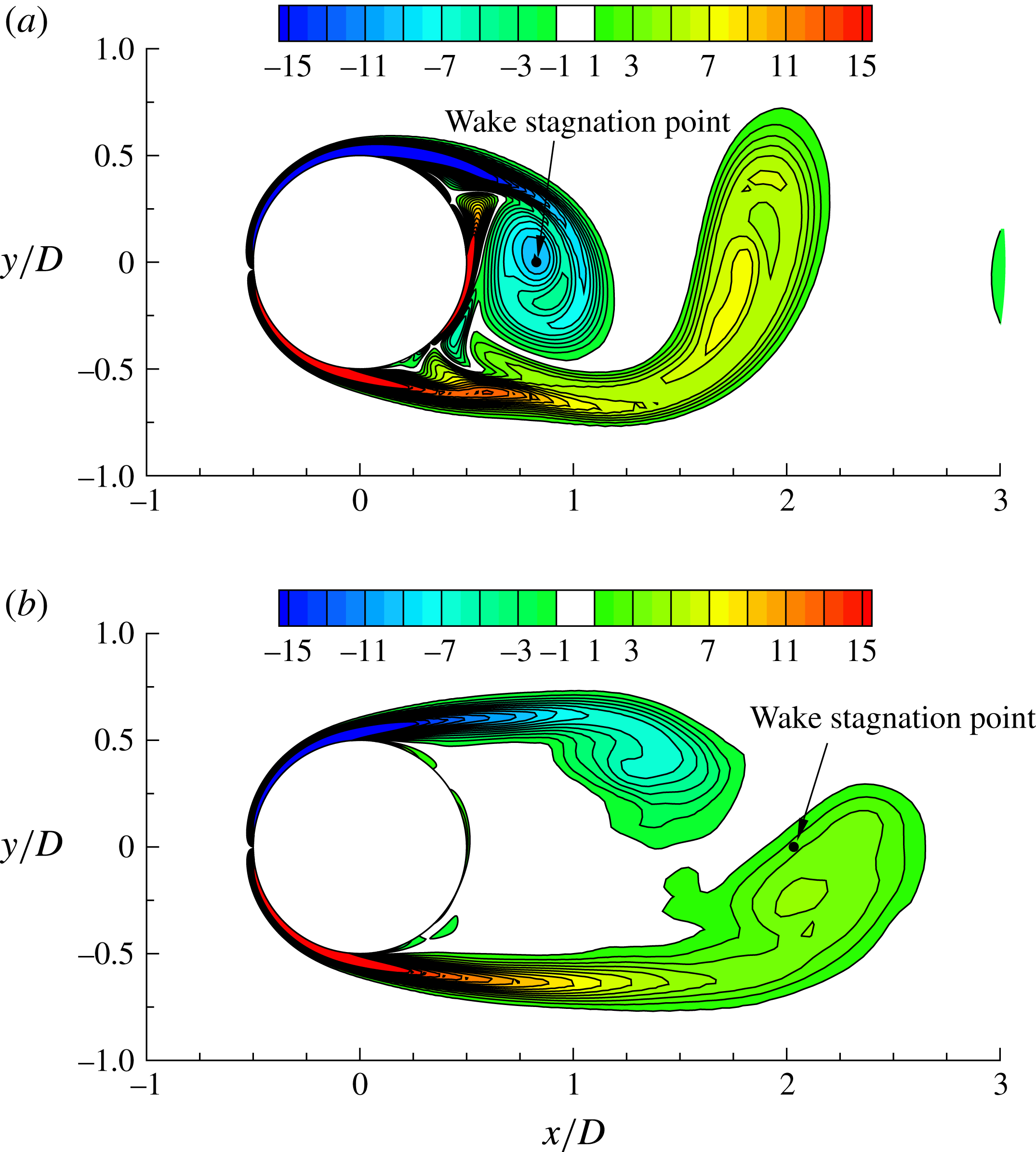
. Figure 7 shows the instantaneous
 $\unicode[STIX]{x1D714}_{z}$
contours of the 2D and 3D (averaged over the span) flows at
 $Re=1000$
, at the time instant that the maximum
 $u_{x}$
at
 $x/D=0$
is the largest on the upper side of the cylinder and the smallest on the lower side of the cylinder, namely at the instant when
 $u_{x}$
on the lower side of the cylinder starts to increase. At this point, a positive vortex has just been shed from the lower shear layer, and the lower shear layer is about to roll up to form a new vortex. As shown in figure 7(a), the shedding of the positive vortex in the 2D flow is to a great extent influenced by the rolling up of the negative vortex from the opposite side of the cylinder. For the 3D flow, however, as the recirculation region is much longer (as indicated by the wake stagnation point in figure 7), the lower separating shear layer becomes longer and thus weaker at the point of shedding (figure 7
b). Therefore, the positive vortex in the 3D flow is shed more independently, at a point that the negative vortex from the opposite side of the cylinder is still relatively far away from the lower shear layer. In other words, the cross-flow distance for the negative vortex to roll up to trigger the shedding of the positive vortex is reduced. Consequently, the vortex shedding frequency of the 3D flow would scale on a length smaller than that for the 2D flow. When
 $D^{\prime }$
is used for the determination of both
 $St_{2D}^{\ast }$
and
 $St_{3D}^{\ast }$
,
 $St_{3D}^{\ast }$
would be larger than
 $St_{2D}^{\ast }$
, as is manifested in figure 2.
Instantaneous
 $\unicode[STIX]{x1D714}_{z}$
contours for flow past a circular cylinder at
 $Re=1000$
: (a) the 2D flow, and (b) the 3D flow (averaged over the span). The wake stagnation point obtained from the time-averaged flow field is marked by a solid dot.

Generally, the deviation between
 $St_{3D}^{\ast }$
and
 $St_{2D}^{\ast }$
is observed at
 $Re>300$
(figure 2), for which the increasing deviation between formation lengths calculated by 2D and 3D DNS (figure 6) gradually becomes a third major factor influencing the vortex shedding frequency.
5 Strouhal numbers for modes A and B
For the laminar regime, which includes mode A and the onset of mode B, an agreement of
 $St_{3D}^{\ast }$
and
 $St_{2D}^{\ast }$
is observed in figure 2, while the difference in the
 $St_{3D}$
and
 $St_{2D}$
values is attributed to the different
 $U_{s}$
and
 $D^{\prime }$
values used for the 2D and 3D flows to transform
 $St^{\ast }$
into the corresponding
 $St$
. This suggests that the drop of
 $St_{3D}$
from its
 $St_{2D}$
counterpart is also due to the decrease in
 $U_{s}$
and the increase in
 $D^{\prime }$
for a 3D flow (figure 3).
The decrease in
 $U_{s}$
in a 3D flow is related to the spanwise energy amplification of the shear layers. The decrease in
 $U_{s}$
also results in a thicker shear layer and thus an increase in
 $D^{\prime }$
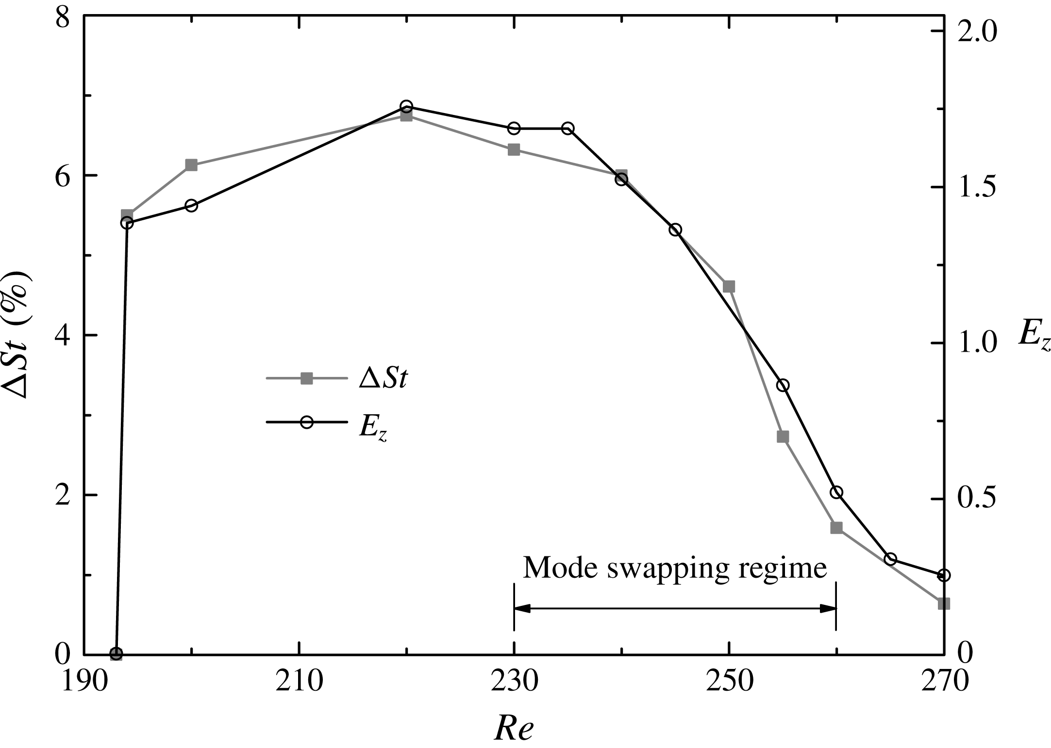
. Therefore, similar variation trends for the degree of deviation between
 $St_{3D}$
and
 $St_{2D}$
and the flow three-dimensionality are observed (figure 8). The deviation between
 $St_{3D}$
and
 $St_{2D}$
is calculated as
 $$\begin{eqnarray}\unicode[STIX]{x0394}St=(St_{2D}-St_{3D})/St_{2D}\times 100\,\%.\end{eqnarray}$$
The flow three-dimensionality is represented by the statistically stationary spanwise kinetic energy
 $E_{z}$
integrated over the near-wake region of
 $x/D=0{-}10$
, where
 $E_{z}$
is defined as
 $$\begin{eqnarray}E_{z}=\frac{1}{2}\int _{V}(u_{z}/U)^{2}\,\text{d}V,\end{eqnarray}$$
where
 $V$
is the volume of the flow field of interest.
Variation trends for the degree of deviation between
 $St_{3D}$
and
 $St_{2D}$
(
 $\unicode[STIX]{x0394}St$
) and the flow three-dimensionality (represented by
 $E_{z}$
).

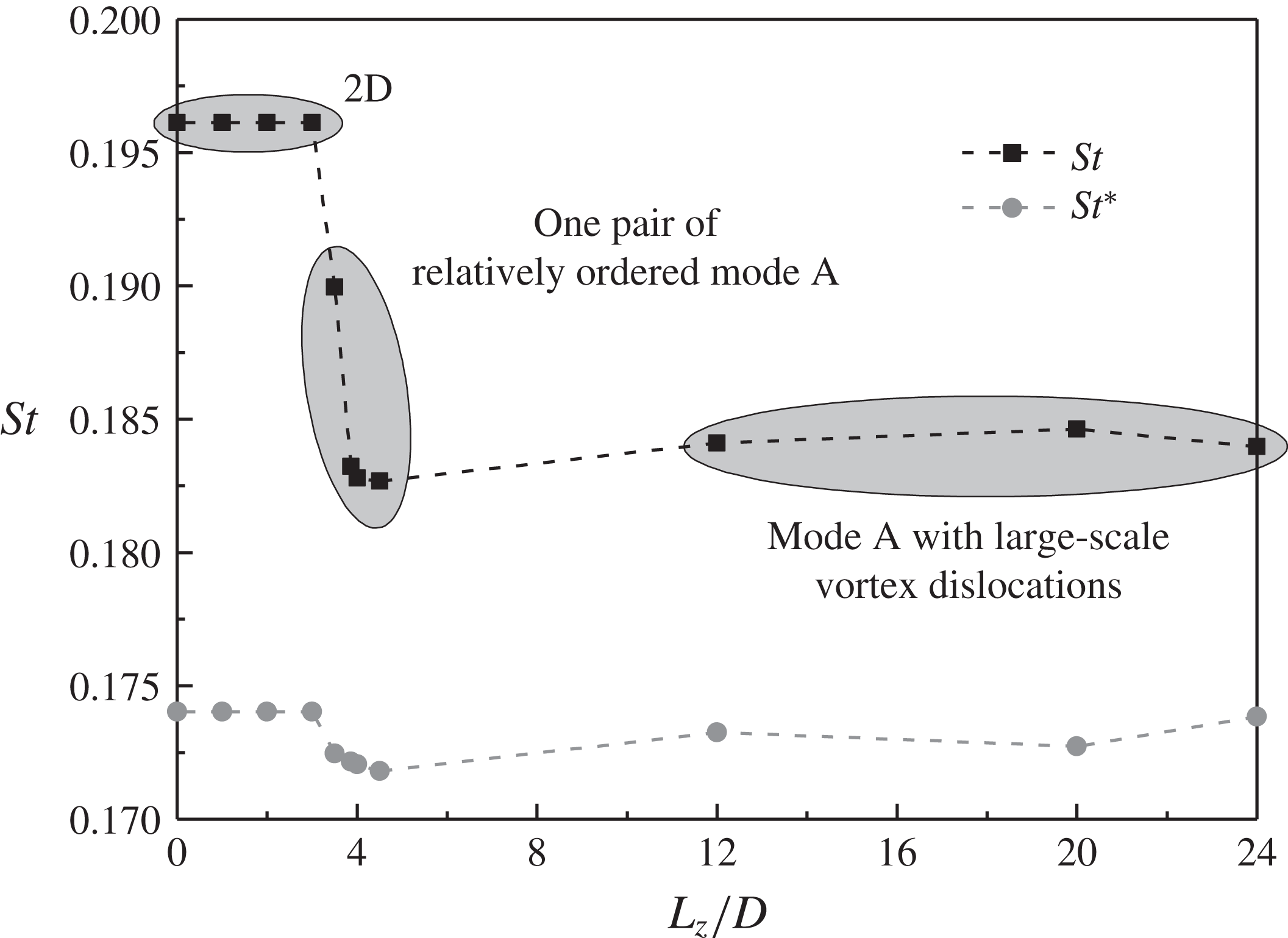
The Strouhal number for the mode A flow is further studied at
 $Re=200$
through varying the cylinder span length
 $L_{z}$
to obtain different mode A flow structures. The variation of
 $St$
with
 $L_{z}$
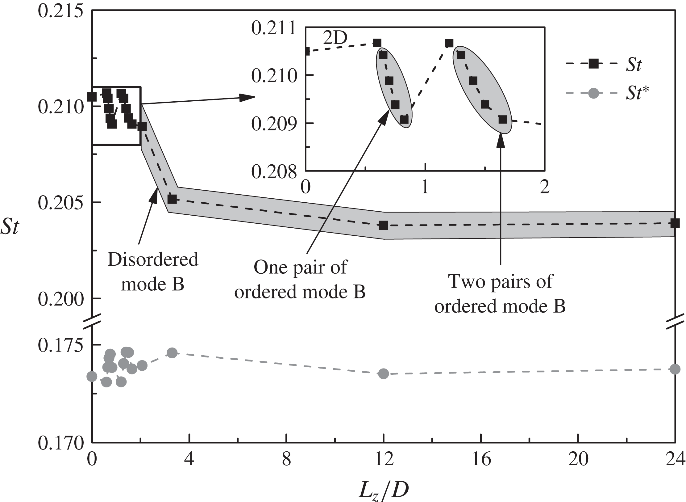
is shown in figure 9. The flow is 2D for
 $L_{z}/D\leqslant 3$
but becomes unstable to mode A instability for
 $L_{z}/D\geqslant 3.5$
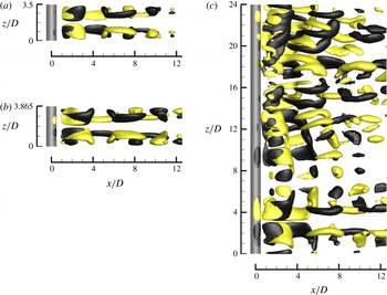
, which is consistent with the neutral instability curve for mode A proposed by Barkley & Henderson (Reference Barkley and Henderson1996). Figure 10 shows some typical mode A wake flow structures in the fully developed state, identified by the isosurfaces of the streamwise vorticity
 $\unicode[STIX]{x1D714}_{x}$
:
 $$\begin{eqnarray}\unicode[STIX]{x1D714}_{x}=\left(\frac{\unicode[STIX]{x2202}u_{z}}{\unicode[STIX]{x2202}y}-\frac{\unicode[STIX]{x2202}u_{y}}{\unicode[STIX]{x2202}z}\right)\frac{D}{U}.\end{eqnarray}$$
For
 $L_{z}/D\geqslant 12$
, the fully developed flow is represented by mode A with large-scale vortex dislocations (e.g. figure 10
c), which is consistent with the experimental results (e.g. Williamson Reference Williamson1996a
). In contrast, for
 $L_{z}$
comparable to the most unstable spanwise wavelength of mode A of
 $\unicode[STIX]{x1D706}_{A}=3.865D$
at
 $Re=200$
, the fully developed flow is represented by one pair of ordered mode A structures (e.g. figure 10
a,b), while vortex dislocation is suppressed due to the confinement of a short span length (Henderson Reference Henderson1997).
Variation of
 $St$
with
 $L_{z}$
for the mode A flow at
 $Re=200$
.

Mode A wake flow structures in the fully developed state at
 $Re=200$
: (a) with
 $L_{z}/D=3.5$
, (b) with
 $L_{z}/D=3.865$
and (c) with
 $L_{z}/D=24$
. The wake structures are captured by the isosurfaces of
 $\unicode[STIX]{x1D714}_{x}=\pm 0.5$
. Dark grey and light yellow denote positive and negative values, respectively. The flow is from the left to the right past the cylinder on the left.

Based on the observation of an obvious drop of
 $St_{3D}$
with the development of ordered mode A structures under the restriction of
 $L_{z}=\unicode[STIX]{x1D706}_{A}$
at
 $Re=195$
, Henderson (Reference Henderson1997) suggested that the drop of
 $St_{3D}$
is due to the existence of the pure mode A structure rather than vortex dislocation. This is consistent with the present results at
 $Re=200$
shown in figures 9 and 10, where the
 $St_{3D}$
value for
 $L_{z}=\unicode[STIX]{x1D706}_{A}=3.865D$
(with pure mode A) is very close to those for
 $L_{z}\geqslant 12D$
(with dislocations). However, for the pure mode A flow calculated with
 $L_{z}=3.5D$
(figure 10
a), the
 $St_{3D}$
value is not in line with those for
 $L_{z}=3.865D$
or
 $L_{z}\geqslant 12D$
. This cannot be explained by Henderson’s (Reference Henderson1997) argument.
As shown in figure 9, although the vortex structures and
 $St$
may be different for the cases with different
 $L_{z}$
, the
 $St^{\ast }$
values are quite uniform. This suggests that the drop of
 $St_{3D}$
is largely due to the decrease in
 $U_{s}$
and the increase in
 $D^{\prime }$
for a 3D flow, rather than the existence of a particular wake structure such as pure mode A or vortex dislocation.
The same mechanism also holds for the Strouhal number for the mode B flow. The mode B flow is analysed at
 $Re=300$
rather than at the onset of wake turbulence of
 $Re=270$
because at
 $Re=300$
an obvious drop of
 $St_{3D}$
is observed while the deviation between
 $St_{3D}^{\ast }$
and
 $St_{2D}^{\ast }$
is still negligibly small (figure 2). Figure 11 shows the variation of
 $St$
with
 $L_{z}$
for the mode B flow at
 $Re=300$
. The wake flow is represented by one or two pairs of ordered mode B structures at small
 $L_{z}$
(e.g. figure 12
a–c) but becomes disordered at large
 $L_{z}$
(e.g. figure 12
d). Similar to the results of the mode A flow shown in figure 9, the
 $St^{\ast }$
values shown in figure 11 for the mode B flow are also quite uniform, regardless of the different vortex structures and
 $St$
values under different
 $L_{z}$
.
Variation of
 $St$
with
 $L_{z}$
for the mode B flow at
 $Re=300$
.

Mode B wake flow structures in the fully developed state at
 $Re=300$
with (a)
 $L_{z}/D=0.65$
, (b)
 $L_{z}/D=0.825$
, (c)
 $L_{z}/D=1.65$
and (d)
 $L_{z}/D=24$
. The wake structures are captured by the isosurfaces of
 $\unicode[STIX]{x1D714}_{x}=\pm 0.5$
. Dark grey and light yellow denote positive and negative values, respectively. The flow is from the left to the right past the cylinder on the left.

6 Conclusions
This paper examines both the 2D and 3D
 $St{-}Re$
relationships for flow past a circular cylinder in the low
 $Re$
range of
 $Re\leqslant 1000$
through DNS. An improved method is proposed for the determination of the separating velocity
 $U_{s}$
and the wake width
 $D^{\prime }$
to allow for a better estimation of the wake Strouhal number
 $St^{\ast }$
.
Based on 2D DNS, it is found that the
 $St_{2D}^{\ast }$
values for
 $Re$
in the extended laminar regime are more uniform than the original
 $St_{2D}$
values, since the 2D vortex shedding frequency scales primarily on
 $U_{s}$
and
 $D^{\prime }$
. Based on 3D DNS, it is found that
 $St_{3D}^{\ast }$
matches
 $St_{2D}^{\ast }$
well for the laminar regime of
 $Re$
up to approximately 270. However, as the wake flow becomes increasingly turbulent with further increase in
 $Re$
,
 $St_{3D}^{\ast }$
increases gradually and deviates from the corresponding
 $St_{2D}^{\ast }$
value. This is because the increase in the streamwise length of the recirculation region results in a weaker separating shear layer at the point of vortex shedding, such that vortex shedding is less influenced by the rolling up of the vortex from the opposite side of the cylinder. Owing to a reduced cross-flow distance for the vortex from the opposite side of the cylinder to roll up to trigger vortex shedding, the vortex shedding frequency scales on a length that is smaller than
 $D^{\prime }$
.
For both the mode A and mode B flows in the laminar regime, in addition to the agreement of
 $St_{2D}^{\ast }$
and
 $St_{3D}^{\ast }$
by using a relatively large cylinder span length of
 $L_{z}=12D$
, uniform
 $St^{\ast }$
values are also obtained by using different
 $L_{z}$
, regardless of the different wake structures and
 $St$
due to the restriction of
 $L_{z}$
. This suggests that the drop of
 $St_{3D}$
from
 $St_{2D}$
with the development of different 3D wake structures is due to the decrease in the separating velocity and the increase in the wake width for a 3D flow, rather than the existence of a particular wake structure such as pure mode A or vortex dislocation.
Acknowledgements
The corresponding author (L.C.) would like to acknowledge the support from the National Natural Science Foundation of China (grant ID 51479025) and the authors would like to acknowledge the Pawsey Supercomputing Centre for providing the computing resources with funding from the Australian Government and the Government of Western Australia.
Appendix A. Mesh convergence
The time step
 $\unicode[STIX]{x0394}t$
adopted for each case is based on the criterion that the maximum Courant number (
 $Co_{max}$
) in the computational domain is kept below 0.4. The Courant number for a cell is defined as
 $$\begin{eqnarray}Co=|u|\unicode[STIX]{x0394}t/\unicode[STIX]{x0394}l,\end{eqnarray}$$
where
 $|u|$
is the magnitude of the velocity through a cell, and
 $\unicode[STIX]{x0394}l$
is the cell size in the direction of the velocity.
A mesh dependence study on the refined 2D mesh is carried out at
 $Re=1000$
(the largest
 $Re$
adopted in this study) with the following three variations.
-
(1) Increase in the domain size. The distance from the cylinder centre to each side of the domain is increased from
$30D$
to
$60D$
. -
(2) Increase in the mesh resolution. The number of cells in both
$x$
and
$y$
directions is doubled. In particular, the number of nodes around the cylinder surface is doubled from 240 to 480, and the height of the first layer of mesh next to the cylinder surface is halved from
$2.315\times 10^{-4}D$
to
$1.174\times 10^{-4}D$
. -
(3) Decrease in the time step size. The time step size is reduced to 20 % of that before through keeping
$Co_{max}$
below 0.08.


The mesh convergence is checked by examining the variations in the hydrodynamic forces on the cylinder. The hydrodynamic forces, including the drag and lift force coefficients (
 $C_{D}$
and
 $C_{L}$
), the Strouhal number (
 $St$
) and the base pressure coefficient (
 $C_{pb}$
) are defined as follows:
 $$\begin{eqnarray}\displaystyle & \displaystyle C_{D}=F_{D}/(\unicode[STIX]{x1D70C}DU^{2}L_{z}/2), & \displaystyle\end{eqnarray}$$
 $$\begin{eqnarray}\displaystyle & \displaystyle C_{L}=F_{L}/(\unicode[STIX]{x1D70C}DU^{2}L_{z}/2), & \displaystyle\end{eqnarray}$$
 $$\begin{eqnarray}\displaystyle & \displaystyle St=\,f_{L}D/U, & \displaystyle\end{eqnarray}$$
 $$\begin{eqnarray}\displaystyle & \displaystyle C_{pb}=(p_{b}-p_{\infty })/(\unicode[STIX]{x1D70C}U^{2}/2), & \displaystyle\end{eqnarray}$$
where
 $F_{D}$
and
 $F_{L}$
are the integrated drag force and lift force on the cylinder, respectively,
 $L_{z}$
is the spanwise domain length,
 $f_{L}$
is the frequency of the fluctuating lift force,
 $p_{b}$
is the time-averaged pressure at the rear stagnation point of the cylinder and
 $p_{\infty }$
is the reference pressure at the inlet of the domain. The time-averaged drag and lift coefficients are denoted as
 $\overline{C_{D}}$
and
 $\overline{C_{L}}$
, respectively. The root-mean-square lift coefficient
 $C_{L}^{\prime }$
is defined as
 $$\begin{eqnarray}C_{L}^{\prime }=\sqrt{\frac{1}{N}\mathop{\sum }_{i=1}^{N}(C_{L,i}-\overline{C_{L}})^{2}},\end{eqnarray}$$
where
 $N$
is the number of values in the time history of
 $C_{L}$
.
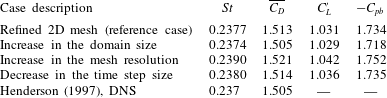
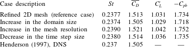
The results of the 2D mesh dependence study are listed in table 2. With respect to the reference case with the refined 2D mesh, the largest variations in the hydrodynamic forces for the three variation cases are approximately 1 %. In addition, the
 $St$
and
 $\overline{C_{D}}$
values calculated with the refined 2D mesh are very close to those calculated by Henderson (Reference Henderson1997). The above results suggest that the refined 2D mesh is adequate for the present study with
 $Re\leqslant 1000$
.
Results of the 2D mesh dependence study at
 $Re=1000$
.
Results of the 3D mesh dependence study at
 $Re=1000$
.
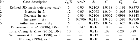
The 3D mesh dependence study focuses on the mesh resolution and domain size in the spanwise direction. The reference case for the 3D mesh dependence study is the refined 3D mesh, which is formed by replicating the refined 2D mesh along the
 $z$
-axis with
 $L_{z}/D=6$
and a uniform spanwise cell length of
 $\unicode[STIX]{x0394}z/D=0.05$
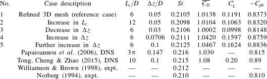
. Table 3 lists the numerical cases and results for the 3D mesh dependence study at
 $Re=1000$
. At least 800 non-dimensional time units (defined as
 $t^{\ast }=Ut/D$
) of the fully developed flow are used to calculate the statistical stationary hydrodynamic forces on the cylinder. The
 $St$
value for the 3D flow is determined using the peak frequency derived from the FFT of the time history of the lift coefficient.
With respect to the reference case (case 1) in table 3, case 2 is designed to examine the adequacy of
 $L_{z}$
. It is found that an
 $L_{z}$
of
 $6D$
is sufficient for the simulation at
 $Re=1000$
, since an increase in
 $L_{z}$
to
 $12D$
results in very close numerical results. Note that
 $C_{L}^{\prime }$
may decrease to a small extent, since with increasing
 $L_{z}$
the integrated lift coefficient is more likely to be cancelled out by the phase differences along the span (Henderson Reference Henderson1997). On the other hand, cases 3–5 are designed to examine the influence of
 $\unicode[STIX]{x0394}z$
. Relatively small variations of the hydrodynamic forces are observed when
 $\unicode[STIX]{x0394}z$
decreases from
 $0.1D$
to
 $0.0706D$
(case 5 to case 4) and from
 $0.05D$
to
 $0.03D$
(case 1 to case 3), whereas more dramatic variations of the hydrodynamic forces are observed when
 $\unicode[STIX]{x0394}z$
decreases from
 $0.0706D$
to
 $0.05D$
(case 4 to case 1). As a compromise between numerical accuracy and computational cost, the reference case with
 $\unicode[STIX]{x0394}z/D=0.05$
(case 1 in table 3) is adopted for the 3D simulations in this study for
 $Re=400{-}1000$
. It is also seen in table 3 that the hydrodynamic forces predicted with the reference case are in close agreement with the experimental results reported in Norberg (Reference Norberg1994) and Williamson & Brown (Reference Williamson and Brown1998).
While it was demonstrated in Jiang et al. (Reference Jiang, Cheng, Draper, An and Tong2016) that the standard 3D mesh with
 $\unicode[STIX]{x0394}z/D=0.1$
is adequate for
 $Re\leqslant 300$
, the cases listed in table 3 suggest that at least
 $\unicode[STIX]{x0394}z/D=0.05$
is required for
 $Re=1000$
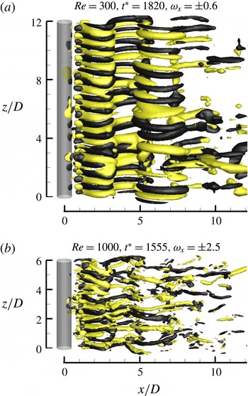
. As shown in figure 13, this is because the streamwise vortices of mode B become finer with increasing
 $Re$
, and therefore a finer mesh resolution in the spanwise direction, namely a smaller
 $\unicode[STIX]{x0394}z$
, is required to resolve the finer mode B structures. The decrease of the
 $\overline{C_{D}}$
,
 $C_{L}^{\prime }$
and
 $-C_{pb}$
values as
 $\unicode[STIX]{x0394}z/D$
decreases from
 $0.0706D$
to
 $0.05D$
(table 3) is also due to a refined resolution of the mode B structures and consequently an increase in the flow three-dimensionality. Consistently, for the DNS results reported in Tong et al. (Reference Tong, Cheng and Zhao2015) by using a very similar numerical formulation to that adopted in the present study, the use of
 $\unicode[STIX]{x0394}z/D=0.1$
for
 $Re=1000$
resulted in overpredicted
 $\overline{C_{D}}$
,
 $C_{L}^{\prime }$
and
 $-C_{pb}$
values (table 3).
Isosurfaces of
 $\unicode[STIX]{x1D714}_{x}$
for the fully developed mode B structures at (a)
 $Re=300$
with the standard 3D mesh (
 $L_{z}/D=12$
and
 $\unicode[STIX]{x0394}z/D=0.1$
), and (b)
 $Re=1000$
with the refined 3D mesh (
 $L_{z}/D=6$
and
 $\unicode[STIX]{x0394}z/D=0.05$
). Dark grey and light yellow denote positive and negative values, respectively. The flow is from the left to the right past the cylinder on the left.

By using the refined 3D mesh as a replacement for the standard 3D mesh for
 $Re>300$
, the number of spanwise mesh layers per unit span length is doubled. This was the incentive for the use of a halved
 $L_{z}$
of
 $6D$
for the refined 3D mesh so as to keep the computational cost at an affordable level. For
 $Re<270$
, due to the existence of the relatively large-scale mode A structure (with a spanwise wavelength of
 ${\sim}4D$
) and the associated vortex dislocation,
 $L_{z}>10D$
is necessary for the prediction of converged numerical results (Jiang, Cheng & An Reference Jiang, Cheng and An2017c
). With further increase in
 $Re$
, the small-scale mode B structure (with a spanwise wavelength of
 ${<}1D$
) becomes the only wake flow mode, which offers theoretical support for the use of a reduced
 $L_{z}$
. This is demonstrated with the 3D mesh dependence study at
 $Re=400$
. As shown in table 4, similar numerical results are obtained when
 $L_{z}/D$
reduces from 12 to 6 (case 3 to case 2 in table 4). In addition, it is found that the numerical results at
 $Re=400$
(case 2 to case 1 in table 4) are less sensitive to the decrease in
 $\unicode[STIX]{x0394}z/D$
from 0.1 to 0.05 than those at
 $Re=1000$
(case 5 to case 1 in table 3), which suggests that
 $\unicode[STIX]{x0394}z/D=0.05$
should also be sufficient for
 $Re=400$
. Hence, in the present study, the refined 3D mesh with
 $L_{z}/D=6$
and
 $\unicode[STIX]{x0394}z/D=0.05$
is adopted for the range of
 $Re=400{-}1000$
for consistency.
Results of the 3D mesh dependence study at
 $Re=400$
.