


1. Introduction
The Taylor–Kolmogorov dissipation scaling is one of the most instructive turbulent theories for homogeneous turbulence. It was first proposed by Taylor (Reference Taylor1935) and later became the cornerstone scaling of the equilibrium cascade, as follows (Kolmogorov Reference Kolmogorov1941):
 \begin{equation} C_\varepsilon=\varepsilon L /{u^3_{rms}}={\rm const.}, \end{equation}
where  $C_\varepsilon$ is the non-dimensional dissipation rate,
 $\varepsilon$ is the dissipation rate of turbulent kinetic energy,
 $L$ is the integral length scale and
 $u_{rms}$ is the root mean square (r.m.s.) of the streamwise velocity fluctuations. We refer to the Taylor–Kolmogorov dissipation scaling as the equilibrium scaling hereafter. Intrinsically, the equilibrium scaling assumes that the process of interscale energy transfer is at equilibrium. This provides fundamental solutions for numerous turbulence models, which are critical for various industrial applications (Pope Reference Pope2001). In the equilibrium scaling and energy cascade framework proposed by Kolmogorov (Reference Kolmogorov1941), the energy spectrum holds an inertial subrange with an exponent of
 $-5/3$, regardless of the different types of flows. Furthermore, combining
 $\varepsilon =15\nu {u_{rms}^2/\lambda }^2$ assuming isotropy (
 $\nu$ is the kinematic viscosity and
 $\lambda$ is the Taylor microscale defined with the streamwise velocity) with (1.1), the equilibrium scaling behaviour can be obtained as
 $L/\lambda = C_\varepsilon Re_\lambda /15 \propto Re_\lambda$, where
 $Re_\lambda = \lambda u_{rms}/\nu$ is the turbulent Reynolds number based on the Taylor microscale.
The equilibrium scaling, i.e. the independence of  $C_\varepsilon$ on
 $Re_\lambda$, is expected and observed for fully developed and statistically stationary, homogeneous and isotropic flows. On the other hand, recent numerical and experimental evidence in more complicated situations such as near field of grid turbulence indicates the existence of the non-equilibrium energy cascade with the new non-equilibrium scaling (Vassilicos Reference Vassilicos2015),
 \begin{equation} C_\varepsilon\sim {Re_0}^{m/2} / {Re_\lambda}^n \left({\neq} {\rm const.}\right), \end{equation}
where  $m \approx n \approx 1$ are the empirical constants and
 $Re_0$ is the global Reynolds number based on a global length scale. Equation (1.2) provides a new non-equilibrium behaviour with the relation (Vassilicos Reference Vassilicos2015)
 \begin{equation} L/\lambda=\frac{C_\varepsilon}{15} Re_\lambda \approx {\rm const.} \end{equation}
The non-equilibrium scaling has been observed in various turbulent flows, including homogenous and inhomogeneous turbulence and shear and shearless flows (Vassilicos Reference Vassilicos2015; Chen et al. Reference Chen, Cuvier, Foucaut, Ostovan and Vassilicos2021). The physical mechanisms of equilibrium and non-equilibrium scalings have been clarified theoretically in the past few years by non-equilibrium correction to the Kolmogorov's  $-5/3$ inertial-range spectrum (Bos & Rubinstein Reference Bos and Rubinstein2017; Wacławczyk et al. Reference Wacławczyk, Nowak, Siebert and Malinowski2022). Bos & Rubinstein (Reference Bos and Rubinstein2017) assumed that the energy spectrum can be decomposed into the
 $-5/3$ equilibrium and
 $-7/3$ non-equilibrium parts, as well as the decompositions of turbulent properties such as
 $\varepsilon$ and
 $C_\varepsilon$. The
 $-7/3$ non-equilibrium spectrum was proposed by Yoshizawa (Reference Yoshizawa1994) for unsteady corrections and was numerically assessed in Horiuti & Tamaki (Reference Horiuti and Tamaki2013). As a consequence, (1.2) with
 $m = n = 15/14$ (for a power-law spectrum extending from the wavenumber
 $k_L$ to
 $k_\eta \gg k_L$, where
 $k_L$ and
 $k_\eta$ are the wavenumbers corresponding to large scale and Kolmogorov scale, respectively) and
 \begin{equation} C_\varepsilon/C_{\varepsilon 0}=(Re_\lambda/Re_{\lambda 0})^{{-}15/14}, \end{equation}
are obtained as an exact form of the non-equilibrium scaling, that stems from the  $-7/3$ non-equilibrium spectrum (Bos & Rubinstein Reference Bos and Rubinstein2017; Wacławczyk et al. Reference Wacławczyk, Nowak, Siebert and Malinowski2022). Here,
 $C_{\varepsilon 0}$ and
 $Re_{\lambda 0}$ are the equilibrium values of
 $C_\varepsilon$ and
 $Re_\lambda$, respectively. They also derived the theoretical expression for the dependence of
 $\lambda /L$ on
 $Re_\lambda$:
 \begin{equation} \lambda/L\sim {Re_\lambda}^{1/14}. \end{equation}
The predicted  $Re_\lambda$ variations of
 $\lambda /L$ are very weak and
 $\lambda /L$ is close to a constant, which is consistent with the empirical relation (1.3) (Bos & Rubinstein Reference Bos and Rubinstein2017; Wacławczyk et al. Reference Wacławczyk, Nowak, Siebert and Malinowski2022). In Bos & Rubinstein (Reference Bos and Rubinstein2017), these theoretical predictions were shown to well predict the unsteady fluctuations of the work of Goto & Vassilicos (Reference Goto and Vassilicos2015) and results of grid turbulence (Valente & Vassilicos Reference Valente and Vassilicos2012). Very recently, the theoretical predictions of (1.4) and (1.5) have been assessed in the atmospheric measurements (Wacławczyk et al. Reference Wacławczyk, Nowak, Siebert and Malinowski2022). The only common characteristic between the two scalings is the Kolmogorov's
 $-5/3$ energy spectrum (Bos & Rubinstein Reference Bos and Rubinstein2017; Alves Portela, Papadakis & Vassilicos Reference Alves Portela, Papadakis and Vassilicos2018). Besides, there appear to be many other factors that affect the dissipation scalings in previous numerical and experimental studies, as summarized below.
Valente & Vassilicos (Reference Valente and Vassilicos2012) found that the non-equilibrium and equilibrium scalings exist in the near and far fields of grid turbulence, respectively. Isaza, Salazar & Warhaft (Reference Isaza, Salazar and Warhaft2014) and Hearst & Lavoie (Reference Hearst and Lavoie2015) indicate that the residual strain is responsible for the non-equilibrium region in the near field of the conventional- and fractal-grid turbulence. Goto & Vassilicos (Reference Goto and Vassilicos2016b) elucidate the dissipation scaling transition period by direct numerical simulations (DNSs) of the decaying periodic turbulence. They reported a critical time at which the dissipation scaling transition occurred and interpreted that the non-equilibrium scaling is observed when both large- and small-scale dissipation rates evolve together.
Melina, Bruce & Vassilicos (Reference Melina, Bruce and Vassilicos2016) studied the effects of vortex shedding from a passive-, fractal- and single-square grid and observed that the vortex shedding influences the derivative statistics and dissipation scaling in the near field. Goto & Vassilicos (Reference Goto and Vassilicos2016b) also confirmed that the effect of large-scale coherent structures on the non-equilibrium scaling cannot be negligible. Alves Portela et al. (Reference Alves Portela, Papadakis and Vassilicos2018) demonstrated that the non-equilibrium scaling exists at the near wake of a square prism if the energy of the large-scale coherent structures is excluded. Bos (Reference Bos2020) estimated the degree of non-equilibrium using a  $k$-
 $\varepsilon$ model and explained the effect of the wakes of the grid bars on the non-equilibrium scaling. The presence of energy in a shear layer behind grid bars (Bos Reference Bos2020) or the presence of a bump at energetic scales in initial energy spectra in homogeneous isotropic turbulence in eddy-damped quasinormal Markovian simulations (Meldi & Sagaut Reference Meldi and Sagaut2018) are shown to be able to reproduce the non-equilibrium scaling.
An important factor influencing the dissipation scaling is the spectral imbalance. Based on ideas from Lumley (Reference Lumley1992), Bos, Shao & Bertoglio (Reference Bos, Shao and Bertoglio2007) showed by a phenomenological model that, in decaying turbulence such as grid turbulence, the energy entering the cascade is not dissipated instantaneously unlike forced turbulence, and this causes the different value of  $C_\varepsilon$ between forced and decaying turbulence even at large Reynolds numbers. Valente, Onishi & da Silva (Reference Valente, Onishi and da Silva2014) claim that the deviations of
 $C_\varepsilon$ from the equilibrium scaling are caused by the imbalance between the nonlinear flux and dissipation. Furthermore, Goto & Vassilicos (Reference Goto and Vassilicos2016a) qualitatively evaluated the relation between the Kolmogorov local equilibrium hypothesis and equilibrium and non-equilibrium dissipation scalings. Their DNS results for high-Reynolds-number turbulence indicate that the invalidity of the equilibrium scaling stems from the collapse of the Kolmogorov local equilibrium hypothesis in the low wavenumber range.
The correlations between the dissipation scaling and periodic force and unsteady turbulence have been found both numerically and experimentally. In Goto & Vassilicos (Reference Goto and Vassilicos2015), DNSs of decaying and forced unsteady spatially periodical turbulence are performed to study the scaling laws for time variations of the energy dissipation rate and interscale energy flux. It is shown that the instantaneous  $C_\varepsilon$ defined with a spatial average in the computational domain follows the same non-equilibrium scaling, while the overall time-averaged
 $C_\varepsilon$ is approximately constant. This is possibly the first study that mentions the difference between instantaneous and long-time-averaged statistics. Previous experimental studies have only shown the long-time-averaged turbulent characteristics along with the streamwise or cross-stream distance, and the difference between long- and short-time-averaged statistics on the dissipation rate has not been investigated in experimental studies.
Although (1.2) with  $m = n = 15/14$ is obtained under the assumptions of homogeneity and isotropy (Bos & Rubinstein Reference Bos and Rubinstein2017), the non-equilibrium scaling (1.2) appears in many types of turbulent flows, regardless of homogeneity (Chen et al. Reference Chen, Cuvier, Foucaut, Ostovan and Vassilicos2021). Also, the values of
 $m$ and
 $n$ in (1.2) could be influenced by the inhomogeneity (Chen et al. Reference Chen, Cuvier, Foucaut, Ostovan and Vassilicos2021). Wacławczyk et al. (Reference Wacławczyk, Nowak, Siebert and Malinowski2022) also pointed out that accounting for the inhomogeneity and anisotropy is the future work for further explaining the non-equilibrium scaling.
So far, experimental studies have focused primarily on the variations of long-time-averaged statistics with various parameters, including the streamwise distance and inlet Reynolds number (Vassilicos Reference Vassilicos2015), while experimental studies of short-time-averaged statistics are blank. Although the physical process of the dissipation scalings has been well understood (Bos & Rubinstein Reference Bos and Rubinstein2017), it has not yet been clear whether the instantaneous (or local) statistics follow the non-equilibrium scalings (1.2)–(1.5) in static- and active-grid turbulence. The related question is whether the streamwise distance affects the dissipation behaviour of the local statistics. To shed light and address the questions mentioned above, we reanalyse the instantaneous velocity signals in the static- and active-grid turbulence in Zheng, Nagata & Watanabe (Reference Zheng, Nagata and Watanabe2021b) and compare the short- and long-time-averaged statistics related with the dissipation. The instantaneous velocity signals in the far field are analysed, where turbulence is quasihomogeneous and isotropic and the long-time-averaged non-dimensional dissipation rate is independent of  $Re_\lambda$. The effect of vortex shedding is small in this region and no bump appears in the energy spectra (Zheng et al. Reference Zheng, Nagata and Watanabe2021b).
The remainder of the paper is organized as follows. In § 2, we describe a new methodology to calculate the long-time-averaged (global) and short-time-averaged (local) statistics. The methodology is applied to hot-wire signals obtained in the static- and active-grid turbulence and the results on the global and local scalings are presented in § 3. Finally, § 4 summarizes the conclusions.
2. Methodology
2.1. Global and local datasets
A new time-dependent analysis of the streamwise fluctuating velocity  $u_{ins}(t)$ of the wind-tunnel experiment has been developed based on the study conducted by Goto & Vassilicos (Reference Goto and Vassilicos2015), which investigated the time variations of the energy dissipation rate in periodic turbulence. The present analysis is also in compliance with Bos & Rubinstein (Reference Bos and Rubinstein2017), in which turbulent properties are decomposed into equilibrium and non-equilibrium parts. Experimental data obtained for the static- and active-grid turbulence in Zheng et al. (Reference Zheng, Nagata and Watanabe2021b) is used for the time-dependent analysis presented in this study. Table 1 lists the forcing mode, the mean rotation rate
 $\varOmega$, the maximum deviations of the rotation rate
 $\omega$, the mean rotation period
 $T$, the maximum deviations of the rotation period
 $t$, the Rossby number
 $R_o$ (
 ${=}U/\varOmega M$:
 $U$ is the mean velocity and
 $M$ is the grid mesh size) and the mesh Reynolds number
 $Re_M$ (
 ${=}UM/\nu$). The experimental set-up, measurements and active-grid forcing protocols have been described in Zheng, Nagata & Watanabe (Reference Zheng, Nagata and Watanabe2021a) and Zheng et al. (Reference Zheng, Nagata and Watanabe2021b). The general procedure for analysing the global and local fluctuating velocity signals and the important parameters associated with the procedure are described as follows.
(i) First, a set of fluctuating velocity signals measured by hot-wire anemometry at a fixed streamwise distance of the test section of the wind tunnel is selected as the global dataset and they are low-pass filtered using the eighth-order Butterworth filter at the Kolmogorov frequency, as conducted by Zheng et al. (Reference Zheng, Nagata and Watanabe2021b). For this global dataset of
 $u_{ins}(t)$, we apply the Reynolds decomposition ($u_{ins}(t) = U + u^\prime (t)$) to extract the mean velocity $U$ and streamwise velocity fluctuations $u^\prime (t)$. For a given global dataset, the sampling time $T$ is determined by the sampling frequency and number. The turbulent characteristics of this global dataset can be found in Zheng et al. (Reference Zheng, Nagata and Watanabe2021b).
(ii) Next, we define a local time scale
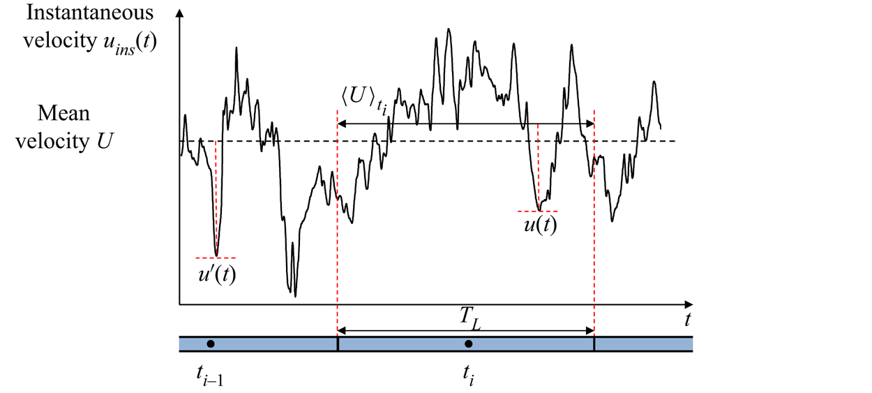
$T_L = C(L/{u_{rms}})$, where $L$ and $u_{rms}$ are obtained from the global dataset and $C$ is an arbitrary constant of order one. The options of $C$ are meaningful because $T_L$ accounts for the order of the eddy turnover time $L/u_{rms}$. The effect of the variation in $C$ on the result is provided in Appendix A. An apposite $C = 0.5$ is chosen such that $C$ is sufficiently small to represent the local datasets and is large enough to extract the information of large-scale motions. Consequently, variations of $u_{ins}(t)$ within $T$ are divided into local datasets whose duration is $T_L$. Figure 1 illustrates an example of the global and local datasets. The number of the local dataset $n$ is obtained as an integer of $T/T_L$.(iii) The instantaneous local time
$t_i$ ($i = 1, 2,\ldots, n$) is considered representatively as the centre of each local dataset. Within the short time period $T_L$, we define the local mean velocity $\langle U \rangle _{t_i}$ and fluctuating velocity $u(t) = u_{ins}(t) - \langle U \rangle _{t_i}$, where $\langle \ast \rangle _{t_i}$ denotes a local time average of $\ast$ from $t_i - T_L/2$ to $t_i + T_L/2$ and is given as a function of $t_i$, as described in figure 1. The r.m.s. of velocity fluctuation within $T_L$ is then calculated by $u_{{rms}}(t_i) = \sqrt {\langle u(t)^2 \rangle _{t_i}}$. Hereafter, quantities defined with the local averages are denoted with $(t_i)$. For example, $u_{{rms}}(t_i)$ is the r.m.s. velocity fluctuation calculated with the local average while $u_{{rms}}$ is obtained with the global average. The local time interval $t_i-t_{i-1}$ is equivalent to $T_L$ such that the global dataset is composed of successive local datasets.(iv) To assess the scalings in the local datasets we plot the statistics against the local turbulent Reynolds number
$Re_\lambda (t_i)=u_{rms}(t_i) \lambda (t_i) / \nu$ using a log–log graph. The local Taylor microscale $\lambda (t_i)$ is directly calculated by
(2.1)The entire range of\begin{equation} \lambda^2(t_i) = \frac{{u^2_{rms}}(t_i)}{\langle(\partial u/\partial x)^2\rangle_{t_i}}. \end{equation}$Re_\lambda (t_i)$ is then divided into ten bins of approximately equal width on the log–log graph. Subsequently, $Re_\lambda (t_i)$ in each bin is ensemble-averaged, which is denoted by $\langle \rangle$. The turbulent quantities are also ensemble-averaged within each bin. We eliminate the statistics at the smallest $\langle Re_\lambda (t_i)\rangle$ because of the large scatter owing to a small sample number.


The global and local datasets.

Control parameters.

2.2. Local turbulent characteristics
Next, we calculate the local turbulent characteristics. Assuming that the Taylor frozen hypothesis and isotropy hold in the local datasets, the local dissipation rate  $\varepsilon (t_i)$ and local non-dimensional dissipation rate
 $C_\varepsilon (t_i )$ are calculated as follows:
 $$\begin{gather} \varepsilon(t_i)=15\nu \langle(\partial u/\partial x)^2\rangle_{t_i}, \end{gather}$$
 $$\begin{gather}C_\varepsilon\left(t_i \right) = \frac{\varepsilon\left( t_i\right) L\left(t_i\right)}{{u^3_{rms}}(t_i)}. \end{gather}$$
The validity of the isotropy assumption is discussed in Appendix B. The local integral length scale  $L(t_i)$ is evaluated as
 $L(t_i) = \int _{0}^{r_0} \overline {u(x)u(x+r)} / u_{rms}^2(t_i) \,{\rm d}r$ within a local dataset. Here,
 $r$ is the separation from a position
 $x$,
 $r_0$ is the first zero-crossing point of the autocorrelation function (e.g. Kitamura et al. Reference Kitamura, Nagata, Sakai, Sasoh, Terashima, Saito and Harasaki2014; Zheng et al. Reference Zheng, Nagata and Watanabe2021b) and
 $\bar {\ast }$ denotes an ensemble average of
 $\ast$. The definition of the local integral length scale is the same as the global one: the integration range (for large
 $r$ up to
 $r_0$) can be outside the local dataset. Notice that
 $L(t_i)$ fluctuates by a large amount since it is already very difficult to make it statistically converge with very long time series under Taylor's hypothesis. Thus, we get highly fluctuating quantities such as (2.3) compared with (2.2).
3. Results and discussions
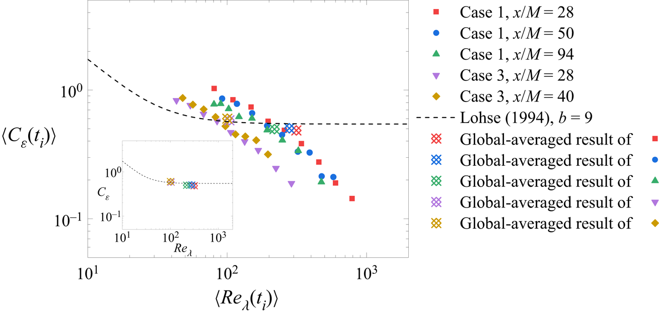
In figure 2,  $\langle C_\varepsilon (t_i)\rangle$ of cases 1 and 3 at different normalized streamwise distances
 $x/M$ are compared in order to assess the scaling law. The profile of
 $C_\varepsilon$ is also shown in the inset. The local values of
 $\langle C_\varepsilon (t_i)\rangle$ in cases 1 and 3 are not constant and decrease with
 $\langle Re_\lambda (t_i) \rangle$ regardless of the variation in
 $x/M$, even when
 $x/M$ is sufficiently large, i.e.
 $x/M = 94$ in active-grid turbulence. On the other hand, the global
 $C_\varepsilon$ (inset of figure 2) tends to be constant and follows the theoretical prediction by Lohse (Reference Lohse1994) with a Kolmogrov constant
 $b = 9$. In previous experimental results of the regular- and fractal-grid turbulence (e.g. Seoud & Vassilicos Reference Seoud and Vassilicos2007; Isaza et al. Reference Isaza, Salazar and Warhaft2014; Nagata et al. Reference Nagata, Saiki, Sakai, Ito and Iwano2017), the global statistics show that the non-equilibrium scaling exists only in the near field. Conversely, the present local-datasets analyses confirm the non-equilibrium scaling locally in the far field of active-grid turbulence. Similar behaviour of the local
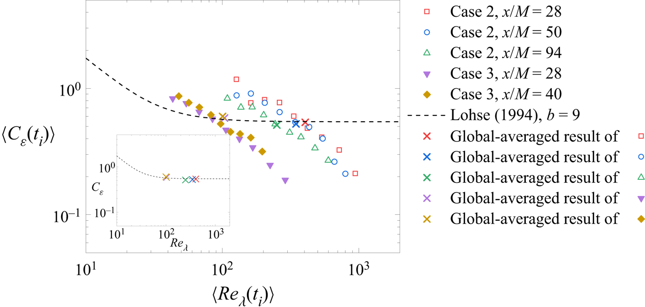
 $\langle C_\varepsilon (t_i)\rangle$ and global
 $C_\varepsilon$ is observed for case 2, as shown in figure 3. Figures 2 and 3 reveal that the local
 $\langle C_\varepsilon (t_i)\rangle$ varies with
 $\langle Re_\lambda (t_i) \rangle$ in all cases regardless of
 $x/M$, while
 $C_\varepsilon \approx$ const. is consistent with previous studies (e.g. Lohse Reference Lohse1994; Zheng et al. Reference Zheng, Nagata and Watanabe2021a). This observation is also consistent with DNS of forced turbulence in Goto & Vassilicos (Reference Goto and Vassilicos2015), which claims that the instantaneous (but spatially averaged inside the box)
 $C_\varepsilon (t)$ approximately follows a power-law decay with
 $Re_\lambda$, and the time-averaged
 $C_\varepsilon$ tends to be constant regardless of the variation in
 $Re_\lambda$.
Variations of  $\langle C_\varepsilon (t_i)\rangle$ with
 $\langle Re_\lambda (t_i) \rangle$ for cases 1 and 3. In the model of Lohse (Reference Lohse1994),
 $b$ is the Kolmogorov constant, which is experimentally known to lie between 6 and 9 (Lohse Reference Lohse1994). The inset shows the global results.

Same as figure 2 but for cases 2 and 3.

Because  $\langle C_\varepsilon (t_i)\rangle$ appears to behave as a power-law function of
 $\langle Re_\lambda (t_i) \rangle$, we further investigate
 $\langle C_\varepsilon (t_i)\rangle$ normalized with the global Reynolds number
 $Re_0$ to assess whether there exists a universal scaling law. In the present study, we define the global Reynolds number as
 $Re_0 = u_{rms}L/\nu$ such that
 $Re_0$ is independent for the different local datasets and is similar to that in Goto & Vassilicos (Reference Goto and Vassilicos2015). To assess the scaling law,
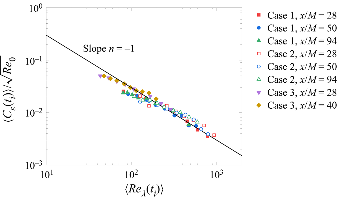
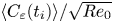
 $\langle C_\varepsilon (t_i)\rangle /\sqrt {Re_0}$ versus
 $\langle Re_\lambda (t_i) \rangle$ is plotted in figure 4. This plot has often been used in previous studies (Goto & Vassilicos Reference Goto and Vassilicos2015; Meldi & Sagaut Reference Meldi and Sagaut2018) and is useful for investigating the non-equilibrium scaling (1.2). Although
 $\langle C_\varepsilon (t_i)\rangle$ takes different values depending on the forcing mode of the active grid and the streamwise location (see figures 2 and 3),
 $\langle C_\varepsilon (t_i)\rangle /\sqrt {Re_0}$ of cases 1, 2 and 3 collapse very well regardless of
 $x/M$, especially for
 $\langle Re_\lambda ( t_i) \rangle \gtrsim 200$. The nonlinear fit with the Levenberg–Marquardt algorithm yields a power-law exponent of
 $-0.87 \pm 0.04$ in this range. The result further proves that the non-equilibrium scaling (1.2) with
 $m \approx n \approx 1$ holds for local statistics even in the far field of grid turbulence. The present results are also within error-bars indistinguishable from the theoretical value
 $m = n = 15/14$ in Bos & Rubinstein (Reference Bos and Rubinstein2017). Note that
 $Re_0$ is a constant in each dataset and the slope close to
 $-1$ is not a trivial result owing to the normalization. On the other hand, figure 4 suggests that the profiles of
 $\langle C_\varepsilon (t_i)\rangle /\sqrt {Re_0}$ of cases 1, 2 and 3 deviate from the non-equilibrium scaling at low
 $\langle Re_\lambda (t_i) \rangle$. The tendency is consistent with Goto & Vassilicos (Reference Goto and Vassilicos2015), in which the instantaneous value of
 $C_\varepsilon (t)$ is nearly constant as
 $Re_\lambda$ decays in the decaying turbulence.
Plot of  $\langle C_\varepsilon (t_i )\rangle /\sqrt {Re_0}$ versus
 $\langle Re_\lambda ( t_i) \rangle$ in cases 1, 2 and 3. The solid line represents
 $\langle C_\varepsilon (t_i )\rangle /\sqrt {Re_0} \propto \langle Re_\lambda ( t_i) \rangle ^n$ with
 $n = -1$.

The global behaviour of  $L/\lambda$ versus
 $Re_M$,
 $Re_\lambda$ and
 $x/M$ has been investigated in previous studies to further investigate the non-equilibrium scaling (e.g. Valente & Vassilicos Reference Valente and Vassilicos2011, Reference Valente and Vassilicos2012; Hearst & Lavoie Reference Hearst and Lavoie2014; Nagata et al. Reference Nagata, Saiki, Sakai, Ito and Iwano2017). The equilibrium scaling (1.1) leads to
 $L/\lambda = C_\varepsilon Re_\lambda /15 \propto Re_\lambda$, whereas the non-equilibrium scaling (1.2) implies that
 $L/\lambda \approx$ const. Actually, these profiles for non-equilibrium turbulence have been observed in different types of grid turbulence (Valente & Vassilicos Reference Valente and Vassilicos2011, Reference Valente and Vassilicos2012). Bos & Rubinstein (Reference Bos and Rubinstein2017) has obtained the theoretical expression for
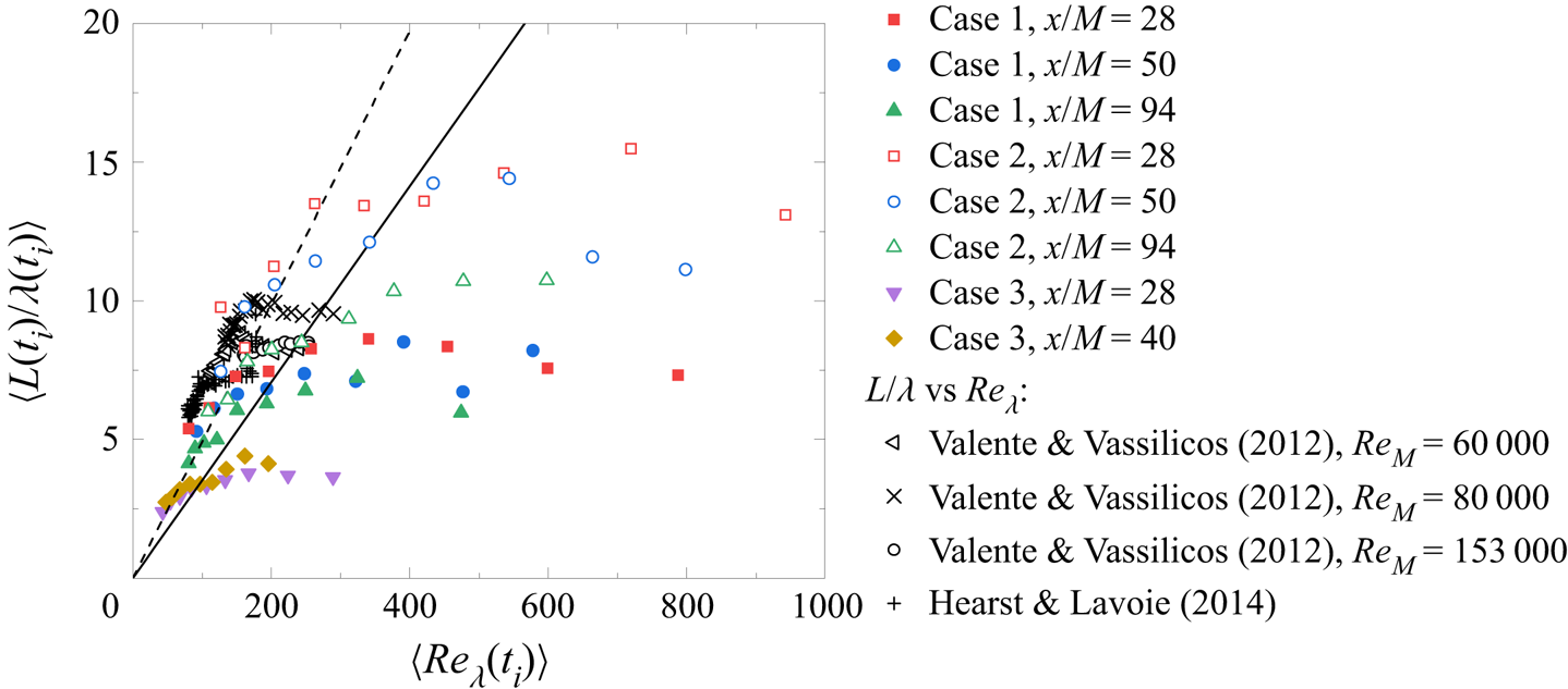
 $\lambda /L$ (1.5), which is close to a constant. Figure 5 plots the local
 $\langle L(t_i)/\lambda (t_i)\rangle$ as a function of
 $\langle Re_\lambda (t_i)\rangle$. Previous global results of
 $L/\lambda$ with different
 $Re_M$ in fractal- and passive-grid turbulence are also plotted as a function of
 $Re_\lambda$ for reference. The values of
 $\langle L(t_i)/\lambda (t_i)\rangle$ in cases 1 and 2 are larger than those of case 3 because the active-grid turbulence generates a larger integral length scale. For all the cases,
 $\langle L(t_i)/\lambda (t_i)\rangle$ has a region dependent on
 $\langle Re_\lambda (t_i)\rangle$ at
 $\langle Re_\lambda (t_i)\rangle \lesssim 200$. The slopes show the equilibrium scaling
 $\langle L(t_i)/\lambda (t_i)\rangle = C_\varepsilon \langle Re_\lambda (t_i)\rangle /15$ with the global values of
 $C_\varepsilon = 0.53$ and
 $0.74$ for cases 1 and 3, respectively. It has been proved in figure 5 that
 $\langle L(t_i)/\lambda (t_i)\rangle$ in the
 $\langle Re_\lambda (t_i)\rangle$-dependent region is consistent with the equilibrium scaling behaviour. However, as
 $\langle Re_\lambda (t_i)\rangle$ further increases, there appears a trend in all the three cases where
 $\langle L(t_i)/\lambda (t_i)\rangle$ is independent of
 $\langle Re_\lambda (t_i)\rangle$, which is consistent with the global results of previous studies (Valente & Vassilicos Reference Valente and Vassilicos2012; Hearst & Lavoie Reference Hearst and Lavoie2014; Nagata et al. Reference Nagata, Saiki, Sakai, Ito and Iwano2017). The previous data of
 $L/\lambda$ are the global results obtained at different streamwise distances, demonstrating that the dissipation scaling behaves differently in the near and far fields of grid turbulence. The present local results of
 $\langle L(t_i)/\lambda (t_i)\rangle$ prove that the
 $Re_\lambda$-dependency of the equilibrium scaling at low
 $Re_\lambda$ is also established. However, as
 $\langle Re_\lambda (t_i)\rangle$ increases, the non-equilibrium scaling of the local statistics appears and
 $\langle L(t_i)/\lambda (t_i)\rangle$ approaches a constant value, which depends on the global Reynolds number. This equilibrium to non-equilibrium transition of
 $\langle L(t_i)/\lambda (t_i)\rangle$ corresponds to the local results of
 $\langle C_\varepsilon (t_i )\rangle /\sqrt {Re_0}$, where
 $\langle C_\varepsilon (t_i )\rangle /\sqrt {Re_0}$ follows the non-equilibrium scaling at
 $\langle Re_\lambda (t_i)\rangle \gtrsim 200$. Although a dependency on the streamwise distance is observed in the global statistics of different types of turbulence, the local statistics do not respond to the variations in the streamwise distance at least in the far field of grid turbulence. The local observations of this study are evidently different from those presented in figure 10 in Zheng et al. (Reference Zheng, Nagata and Watanabe2021b), in which the global results follow the equilibrium scaling behaviour
 $L/\lambda = C_\varepsilon Re_\lambda /15$ with a constant value of
 $C_\varepsilon$ in both the static- and active-grid turbulence.
Plot of  $\langle L(t_i)/\lambda (t_i)\rangle$ versus
 $\langle Re_\lambda (t_i)\rangle$ for cases 1, 2 and 3, compared with that of global statistics obtained in previous studies. The solid and dashedlines represent
 $\langle L(t_i)/\lambda (t_i) \rangle = C_\varepsilon \langle Re_\lambda (t_i)\rangle /15$ with global values of
 $C_\varepsilon = 0.53$ and
 $0.74$ for cases 1 and 3, respectively.

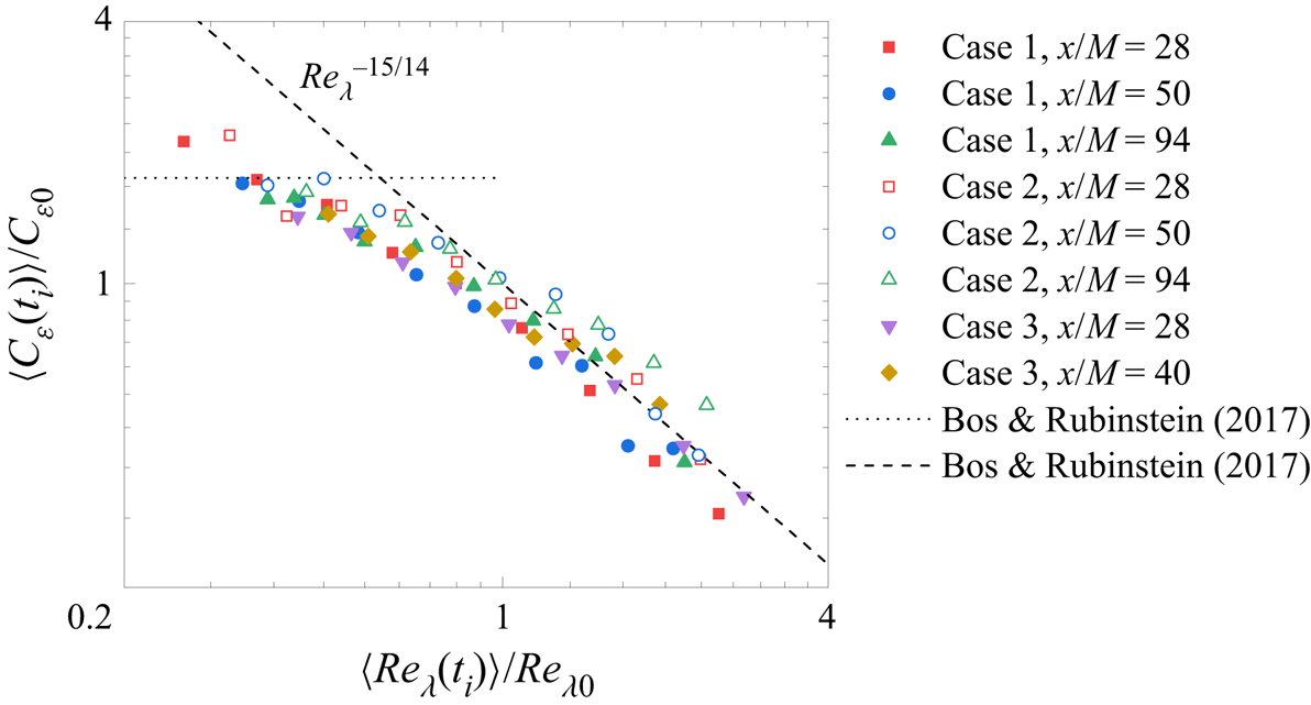
We compare our local results with the theoretical predictions by Bos & Rubinstein (Reference Bos and Rubinstein2017). Figure 6 plots  $\langle C_\varepsilon (t_i)\rangle /C_{\varepsilon 0}$ versus
 $\langle Re_\lambda (t_i)\rangle /Re_{\lambda 0}$. Here,
 $C_{\varepsilon 0}$ and
 $Re_{\lambda 0}$ are equilibrium values of
 $C_\varepsilon$ and
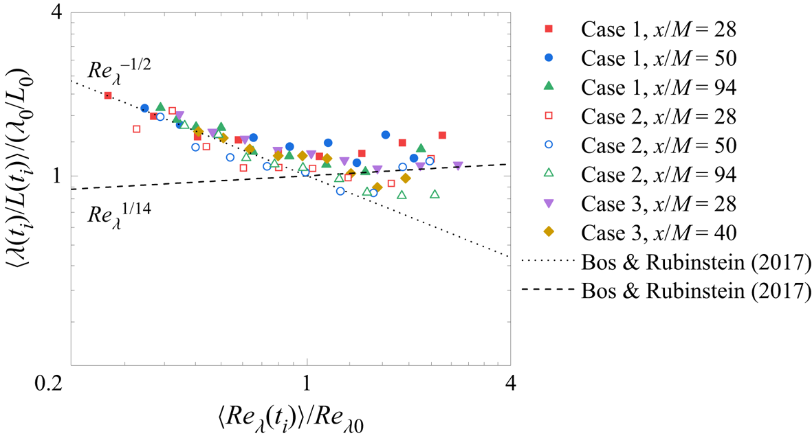
 $Re_\lambda$, respectively, and the global values are used. The present result for the non-dimensional local dissipation rate agrees well with the theoretical predictions. Figure 7 plots
 $\langle \lambda (t_i)/L(t_i)\rangle /(\lambda _0/L_0)$ versus
 $\langle Re_\lambda (t_i)\rangle /Re_{\lambda 0}$. The global values are also used for normalization. Despite the scatter owing to the difficulty in calculating the local statistics, the present results agree well with the theoretical predictions. Note that the lines in figures 6 and 7 do not just represent the slopes but show the exact theoretical expressions. The present results show that the local statistics in grid turbulence also follow the theoretical predictions for non-equilibrium global statistics by Bos & Rubinstein (Reference Bos and Rubinstein2017).
Plot of  $\langle C_\varepsilon (t_i)\rangle /C_{\varepsilon 0}$ versus
 $\langle Re_\lambda (t_i)\rangle /Re_{\lambda 0}$ compared with the theoretical predictions. Here
 $C_{\varepsilon 0}$ and
 $Re_{\lambda 0}$ are equilibrium values of
 $C_\varepsilon$ and
 $Re_\lambda$, respectively, and the global (long-time-averaged) values are used. The dashed and dotted lines represent the expressions (25) and (29) in Bos & Rubinstein (Reference Bos and Rubinstein2017), respectively.

Plot of  $\langle \lambda (t_i)/L(t_i)\rangle /(\lambda _0/L_0)$ versus
 $\langle Re_\lambda (t_i)\rangle /Re_{\lambda 0}$ compared with theoretical predictions.
 $\lambda _0$ and
 $L_0$ are equilibrium values of
 $\lambda$ and
 $L$, respectively, and the global (long-time-averaged) values are used. The dashed and dotted lines represent the expressions (32) and (33) in Bos & Rubinstein (Reference Bos and Rubinstein2017), respectively.

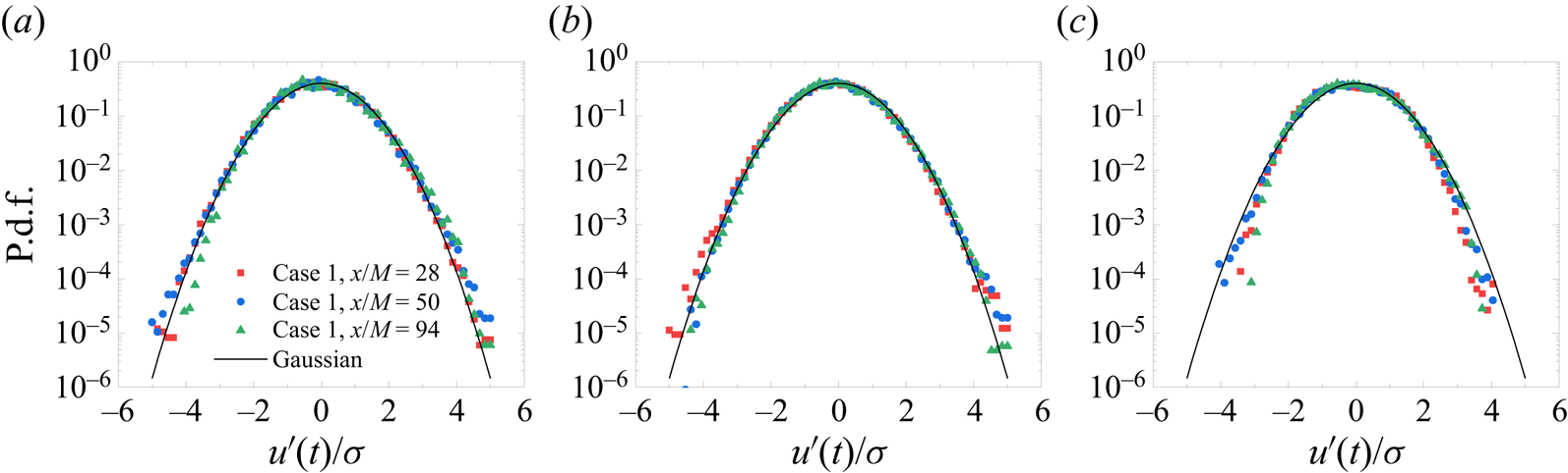
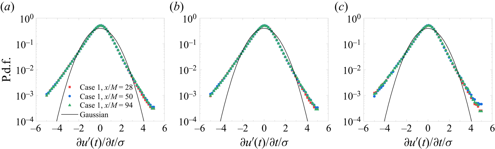
Finally, we calculated the probability density functions (p.d.f.s) of streamwise velocity fluctuations and their time derivatives to see the large- and small-scale intermittency. The unconditional p.d.f., p.d.f.s conditioned on  $\langle Re_\lambda (t_i)\rangle /Re_{\lambda 0} \leqslant 1$ and
 $\langle Re_\lambda (t_i)\rangle /Re_{\lambda 0} > 1$, are shown in figures 8 and 9. Since the local-
 $Re_\lambda$ dependences of
 $\langle C_\varepsilon (t_i)\rangle /C_{\varepsilon 0}$ and
 $\langle \lambda (t_i)/L(t_i)\rangle /(\lambda _0/L_0)$ change depending on
 $\langle Re_\lambda (t_i)\rangle /Re_{\lambda 0} \lesssim 1$ or
 $\langle Re_\lambda (t_i)\rangle /Re_{\lambda 0} \gtrsim 1$ (see figures 6 and 7), we choose
 $\langle Re_\lambda (t_i)\rangle /Re_{\lambda 0} = 1$ as a criterion with which the conditional p.d.f.s apply. Figure 8(a) shows that the p.d.f.s of the unconditional streamwise velocity fluctuations follow the Gaussian distribution regardless of the streamwise distance, as is well known. The conditional p.d.f.s conditioned on the local
 $Re_\lambda$ shown in figures 8(b) and 8(c) also follow the Gaussian distribution. He, Wang & Tong (Reference He, Wang and Tong2018) found non-Gaussian fluctuations with an exponential tail in their p.d.f. of temperature fluctuations in non-equilibrium steady states of turbulent Rayleigh–Bénard convection. Different from their study, velocity fluctuations in the present active-grid turbulence follow the Gaussian distribution even when the local non-dimensional dissipation rate follows the non-equilibrium scaling. The unconditional p.d.f.s of the time derivatives of streamwise velocity fluctuations (figure 9a) qualitatively agree with the data of active-grid turbulence in Makita (Reference Makita1991). It is shown that the p.d.f.s of the time derivatives of streamwise velocity fluctuations do not depend on the local
 $Re_\lambda$ as shown in figures 9(b) and 9(c). These results show that the intermittency of large- and small-scale fluid motions do not depend on the local
 $Re_\lambda$ and streamwise direction considered in the present study. The present study considers the far field of grid turbulence where
 $C_\varepsilon$ is independent of
 $Re_\lambda$. It is interesting to investigate whether the conditional p.d.f.s change depending on the local
 $Re_\lambda$ in the near field, where
 $C_\varepsilon$ follows the non-equilibrium scaling. This is out of the scope of this study and we leave it to future studies.
The p.d.f.s. of the streamwise velocity fluctuations of (a) unconditional global datasets, (b) global datasets with  $\langle Re_\lambda (t_i)\rangle /Re_{\lambda 0} \leqslant 1$ and (c) global datasets with
 $\langle Re_\lambda (t_i)\rangle /Re_{\lambda 0} > 1$. The velocity fluctuations are normalized by each r.m.s. value
 $\sigma$. The solid lines show the Gaussian profile.

The p.d.f.s. of the time derivatives of streamwise velocity fluctuations of (a) unconditional global datasets, (b) global datasets with  $\langle Re_\lambda (t_i)\rangle /Re_{\lambda 0} \leqslant 1$ and (c) global datasets with
 $\langle Re_\lambda (t_i)\rangle /Re_{\lambda 0} > 1$. The velocity derivatives are normalized by each r.m.s. value
 $\sigma$. The solid lines show the Gaussian profile.

4. Conclusions
The dependency of the local statistics on  $Re_\lambda$ has been analysed to assess the non-equilibrium scalings at several streamwise positions of the static- and active-grid turbulence in Zheng et al. (Reference Zheng, Nagata and Watanabe2021b). The global
 $C_\varepsilon$ of the static- and active-grid turbulence follows the equilibrium scaling regardless of the streamwise distance
 $x/M$, in accordance with the previous theoretical results obtained by Lohse (Reference Lohse1994). However, the local non-dimensional dissipation rate
 $\langle C_\varepsilon (t_i)\rangle$ follows the empirical relation (Vassilicos Reference Vassilicos2015) and the theoretical prediction (Bos & Rubinstein Reference Bos and Rubinstein2017) for the non-equilibrium scaling. In particular, as the local characteristics of the static- and active-grid turbulence, the non-equilibrium scaling is even established at the far-downstream distance, whereas it is only found in the near field as the global statistics (Seoud & Vassilicos Reference Seoud and Vassilicos2007; Isaza et al. Reference Isaza, Salazar and Warhaft2014; Nagata et al. Reference Nagata, Saiki, Sakai, Ito and Iwano2017). At small local turbulent Reynolds number
 $\langle Re_\lambda (t_i)\rangle$, local
 $\langle L(t_i)/\lambda (t_i)\rangle$ follows the equilibrium scaling behaviour, as confirmed by previous studies on global statistics. The local
 $\langle L(t_i)/\lambda (t_i)\rangle$ further transitions to the non-equilibrium scaling with increasing
 $\langle Re_\lambda (t_i) \rangle$. The local
 $\langle L(t_i)/\lambda (t_i)\rangle$ also follows the theoretical prediction (Bos & Rubinstein Reference Bos and Rubinstein2017) for non-equilibrium turbulence. These findings further illustrate that for the global statistics, the equilibrium turbulence cascade is only characterized by the turbulent kinetic energy, turbulence dissipation rate and integral length scale. However, for the local statistics, the scaling law changes to the non-equilibrium scaling, which is dependent on the local
 $Re_\lambda$ regardless of the streamwise distance from the grid in the far field. Some previous studies have explained non-equilibrium turbulence based on spectral imbalance, in which the discrepancy locally exists between the scale-by-scale energy transfer at large scales and the dissipation at small scales (Bos et al. Reference Bos, Shao and Bertoglio2007; Valente et al. Reference Valente, Onishi and da Silva2014). Considering these studies, the present results imply that a similar imbalance between the energy transfer and the dissipation may locally exist even if turbulence is globally in an equilibrium state where the energy cascade from large scales balances with the dissipation in terms of time averages. The connection between the global and local non-equilibrium scalings should be futher investigated in future studies.
Acknowledgements
The authors acknowledge three anonymous referees for their useful comments.
Funding
This study is supported by the JSPS KAKENHI (grant nos. 22H01398 and 22K03903) and JSPS bilateral programs no. JPJSBP120219916. Y.Z. was financially supported by the DII collaborative Graduate Program for Accelerating Innovation in Future Electronics and the THERS Interdisciplinary Frontier Next Generation Researcher, Nagoya University.
Declaration of interests
The authors report no conflict of interest.
Appendix A. Dependence of the local $C_\varepsilon$ on $C$


The local time scale  $T_L = C(L/u_{rms})$ affects the estimations of the local turbulent characteristics. The choice of
 $C$ must meet the requirement that the time interval of each local dataset is comparable to eddy turnover time (i.e.
 $C \sim 1$) because the local time average, which works as a low-pass filter, is used to extract local information of large-scale motion. Thus, we investigate the variation of
 $\langle C_\varepsilon (t_i)\rangle$ with different values of
 $C$ (of order one) to find a suitable value of
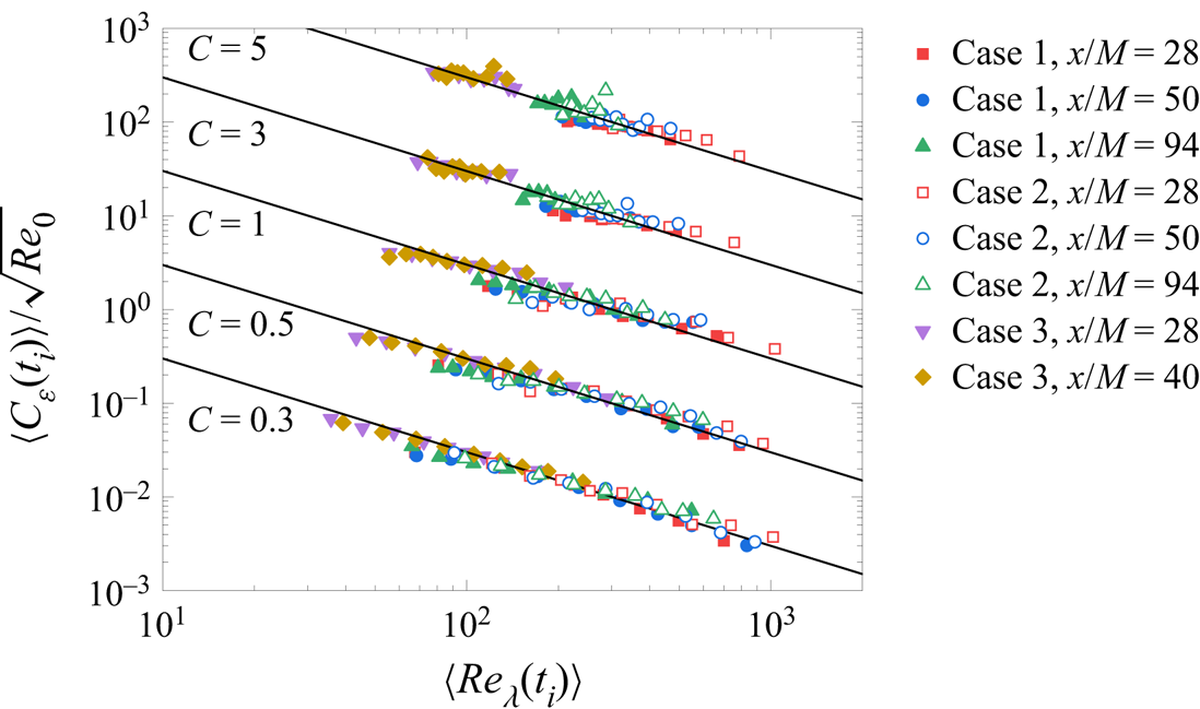
 $C$. Figure 10 plots
 $\langle C_\varepsilon (t_i )\rangle /\sqrt {Re_0}$ against
 $\langle Re_\lambda ( t_i) \rangle$ for
 $C = 0.3, 0.5, 1, 3$ and 5. It is shown that the variation of
 $C$ in this range does not affect the scaling. We conduct all analyses with
 $C = 0.5$ in the present study.
Plot of  $\langle C_\varepsilon (t_i )\rangle /\sqrt {Re_0}$ versus
 $\langle Re_\lambda ( t_i) \rangle$ in cases 1, 2 and 3 with
 $C = 0.3$, 0.5, 1, 3 and 5. Each profile is shifted by a decade for clarity. All solid lines show the power-law exponent
 $-1$.

Appendix B. Isotropy in the local dataset
The isotropy assumption is utilized when calculating the energy dissipation rate in the local datasets. This estimation assumes that the statistics of velocity derivatives defined in each local dataset are isotropic. However, this assumption for the local dataset may not be valid unlike the local isotropy, which is defined with global averages. In the present experiments, only a single component velocity is measured using a single wire for higher spatial resolution than an  $X$ wire. Therefore, we are not able to experimentally evaluate the isotropy in the local datasets. Even if we have two-components velocity data, it is still impossible to assess the validity of estimating the dissipation rate with the isotropy assumption because calculating the dissipation rate without any assumptions requires a full velocity gradient tensor. Therefore, we evaluated the assumption of the statistical isotropy defined for the local datasets using the DNS database of temporally developing grid turbulence (Watanabe & Nagata Reference Watanabe and Nagata2018). The same DNS code has also been applied to stratified grid turbulence with parallel-bar grids (Watanabe, Zheng & Nagata Reference Watanabe, Zheng and Nagata2022). In these DNSs, the flow is initiated by using the wakes of the grid and develops with time. In both kinds of grid turbulence (with square mesh or parallel-bar grids), the basic statistics are shown to be in good agreement with experiments, see Watanabe & Nagata (Reference Watanabe and Nagata2018) and Watanabe et al. (Reference Watanabe, Zheng and Nagata2022). Run Re1a in Watanabe & Nagata (Reference Watanabe and Nagata2018) is used to examine the validity of the isotropic assumption in the analysis of local datasets. The mesh Reynolds number based on the grid mesh size is
 $Re_M = 10\,000$. We choose the non-dimensional time 128, which is equivalent to the streamwise distance
 $x/M = 128$ in experiments. The turbulent Reynolds number
 $Re_\lambda$ is approximately 20. This value of
 $Re_\lambda$ is smaller than those in this study. However, this assessment is still meaningful for the validation of the dissipation estimation because a higher degree of isotropy at small scales is expected for higher
 $Re_\lambda$ in experiments. This is because each local dataset with a size (time) of the integral length (time) scale contains more samples of small-scale motions as
 $Re_\lambda$ increases, resulting in higher local isotropy of the statistics defined in the local dataset. First, we select five
 $x$–
 $y$ slices which are separated in the
 $z$-direction with a distance larger than the longitudinal integral length scale
 $L_{ux}$. Then, each plane is divided into small subdomains with a length of approximately
 $1.03L_{ux}$ in both
 $x$ and
 $y$ directions. A local spatial average
 $\bar {\ast }$ is defined in each subdomain. Then, we calculated
 $v_{rms}/u_{rms}$ (
 $u_{{rms}}$ and
 $v_{{rms}}$ are the r.m.s. of velocity fluctuations
 $u$ and
 $v$),
 $\varepsilon = 2\nu \overline {{\mathsf{s}}_{ij} {\mathsf{s}}_{ji}}$ (
 ${\mathsf{s}}_{ij} = \frac {1}{2}(\partial u_i/\partial x_j + \partial u_j/ \partial x_i)$ is the rate-of-strain tensor of the fluctuating velocities) and
 $\varepsilon _{iso} = 15\nu \overline {(\partial u / \partial x )^2}$ with the assumption that the statistics of velocity gradients defined with the local spatial average is isotropic in each subdomain. The p.d.f.s of
 $v_{rms}/u_{rms}$ and
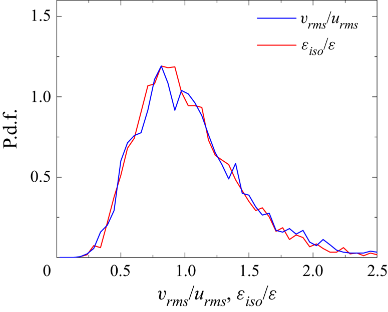
 $\varepsilon _{iso}/\varepsilon$ are shown in figure 11. Both
 $v_{rms}/u_{rms}$ and
 $\varepsilon _{iso}/\varepsilon$ have peaks around 1, suggesting that the statistics defined with each local dataset are close to an isotropic state and the dissipation estimation with
 $\varepsilon _{iso} \sim \varepsilon$ is mostly valid. These results show that the isotropy assumption is reasonably satisfied for local datasets.
The p.d.f. of  $v_{rms}/u_{rms}$ and
 $\varepsilon _{iso}/\varepsilon$.