

With one of the wildest, roughest, and nastiest presidential campaigns in modern American history now thankfully behind us and with late vote returns trickling in to a final official count, it is time to take stock of the 2016 election forecasts. Footnote 1
The Presidential Forecasts
From late June to early September, eight forecasters or teams of forecasters in the PS symposium issued ten presidential election forecasts of the national two-party popular vote (along with the PollyVote composite forecast assembled from an array of different types of forecasts). To avoid any misrepresentation or misunderstanding, it should be emphasized that these forecasts were explicitly of the national two-party popular vote for the major party candidates and not their electoral vote division. Footnote 2
The final vote count indicates 65.9 million votes were cast for Clinton and about 63.0 million for Trump, providing Clinton with a 2.9 million national popular vote plurality. About 7.8 million votes were cast for other candidates. Footnote 3 Despite Trump’s electoral vote victory, Clinton received a narrow but clear plurality of the national popular vote. Footnote 4 Clinton received 51.1% of the two-party popular vote cast nationwide to Trump’s 48.9%.
So, how did these forecasts do? With a few exceptions, the accuracy of the presidential vote forecasts ranged from impressive to extraordinary. In my introduction to the October symposium I described how the models weighed the overall conditions, weak economic performance, and general dissatisfaction with the direction of the nation against the pre-campaign preference polls of the candidates. The former favored the Republicans and the latter favored the Democrats, but all of this was within a context of an open-seat race in a period of polarized hyper-competition. On balance, the forecasts expected a Clinton plurality in a tight race. Summing up, I wrote that “the median forecast predicts that Clinton will win 51.1% of the two-party national vote” (Campbell Reference Campbell2016, 653). This calls for an end-zone celebration. Of course, any forecast or set of forecasts that is this accurate depends a great deal on luck, especially in a year with so many outlandish twists and turns, but one needs to be in that vicinity to be so lucky—and we were.
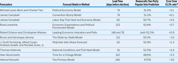
Table 1 presents the individual forecasts and errors from our ten statistically estimated historical-fundamentals models along with the PollyVote composite forecast that draws on alternative prediction methods. Of the forecasts produced by the fundamentals models, three missed Clinton’s national vote share by less than a half of one percentage point! These three forecasts were more accurate than either the median of the flurry of mid-campaign “Polls-Plus” forecasts churned out by Nate Silver’s 538 website or the mean of the 10 pre-election polls gathered by Real Clear Politics on the day before the election. Footnote 5
The Accuracy of the 2016 Presidential Vote Forecasts

Note: The two-party vote for Hillary Clinton was 51.1% as calculated from data made available from official sources gathered by David Wasserman (2016).
Seven of the fundamentals forecasts missed the actual vote percentage by only one percentage point or less. The seven include the forecasts from the Jeromes, Lewis-Beck and Tien, Lockerbie as well as the two forecasts by Erikson and Wlezien and the forecasts from my two models. Just beyond these seven are both Holbrook’s forecast and PollyVote. They missed by just under one and a half percentage points.
Of the 10 forecasts in the collection, only two erred by more than two percentage points. Abramowitz’s “Time for a Change” forecast under-predicted the vote for Clinton by 2.5 percentage points, though he expected as much. In the write-up of his forecast, Abramowitz essentially anticipated a gap between the normal “time for a change” effect and a much less likely “time for a change to Trump” effect. Norpoth’s early March forecast of a 52.5% Trump popular vote majority produced the largest error of the ten forecasts (3.6 percentage points). Footnote 6
Aside from the just noted exceptions, 2016 was a great year for the political science presidential vote forecasts. It provided further evidence that presidential elections can be predicted with a good deal of accuracy well in advance of the election with parsimonious, stable, theoretically grounded, and transparent statistical models based on the historical record of the relationship between the election’s fundamentals and the vote.
So, how did these forecasts do? With a few exceptions, the accuracy of the presidential vote forecasts ranged from impressive to extraordinary.
The Congressional Forecasts
Finally, though the Trump-Clinton contest took center stage (maybe center-ring), important elections were also being conducted for Senate and House seats. Conditions seemed ripe for the Democrats to make big gains in both chambers. Republicans were defending 24 Senate seats to only 10 for the Democrats and Republican numbers in the House (247 seats) were at an 85-year high point. In both chambers, there was plenty of room for Democrats to gain seats and little possibility of Republicans doing better than holding their ground.
The four House and three Senate forecasts reflected this range of possibilities. Although there was speculation during the campaign of a Democratic wave election, it never materialized. Democrats gained only two Senate seats and a mere six House seats. This preserved Republican majorities in both chambers (52 Senate Republicans and 241 House Republicans). Among the House forecasts, Lockerbie and Lewis-Beck and Tien were on target in predicting a preserved status quo. The Abramowitz forecast of a 16 seat Democratic pick-up was a bit high, but my forecast of a 32 seat Democratic seat gain was far off the mark. Among the three Senate forecasts, all expected Democrats to gain more seats than they did. The Abramowitz and the Lewis-Beck and Tien forecasts expected four seat Democratic gains and my forecast was for a seven seat Democratic gain. The errors in different forecasts no doubt reflect differences in each model’s specifications, but the tightness of the presidential race may be a general factor in the failure of Democrats to convert their substantial pre-election exposure advantages (Republicans defending more seats) into actual seat gains.
EARLY AND CERTAIN: THE PROSPECT OF PRESIDENT TRUMP
At first, it sounded outlandish, then, as the general election kicked into high gear, ludicrous, and finally, on the eve of Election Day, downright delusional: the forecast that Donald Trump had an 87-percent chance of being elected President (http://primarymodel.com/). Many who saw this prediction, first posted on March 7, 2016, must have wondered if it was not a misprint. It was Hillary Clinton who had such a high chance of making it to the White House, right? Indeed, the best known websites posting daily election forecasts—from 538, to the Times Upshot, to the Huffington Post, to betting sites like PredicIt—all agreed throughout the election year that Clinton was the prohibitive favorite.
Unlike those forecasts and others featured in PS, the prediction of a near-certain Trump victory did not come from opinion polls or economic indicators. The Primary Model, which generated it, relies solely on election results; in other words, on what voters actually do, not what they say they might do in an election, or on how outside factors might affect their vote. The model distills more than 100 years of presidential elections, primary and general, into a formula with essentially two predictors. One is the performance of the major-party nominees in primaries, the other is the swing of the electoral pendulum in general elections.
Both predictors favored Trump over Clinton. He did better in Republican primaries than she did in Democratic ones, an advantage established in the first two contests (in New Hampshire and South Carolina). And, after two terms of Democratic control of the White House, the electoral pendulum was poised to swing back to the Republican side, especially since Obama’s margin in 2012 was a lot less than it had been in 2008. Given the accuracy of the model, with only one miss among out-of-sample predictions from 1912 to 2012, I had great confidence in the 2016 forecast, no matter how much of an outlier it was.
To be honest, the Primary Model got one thing wrong. Clinton, not Trump, won the popular vote. But, as luck would have it, the predicted popular-vote margin was big enough to guarantee a Trump victory in the Electoral College. Many studies will probe what accounts for the glaring disjuncture between the popular vote and the electoral count in this election. It appears already, though, that Trump won a majority in the Electoral College by capturing three blue states (Pennsylvania, Wisconsin, and Michigan) on top of reliably red states and several battleground states. It is quite telling that the “change” theme strongly resonated in those blue states. When asked in exit polls what candidate quality mattered most, voters in Pennsylvania, Wisconsin, and Michigan picked “bring about change” by a 2–1 margin over having “the right experience.” 2016 was a change election and Trump was the stronger change candidate, especially in the states that decided the outcome.
IT’S THE POPULAR VOTE, STUPID: ELECTORAL COLLEGE MISFIRES AND THE PERILS OF FORECASTING PRESIDENTIAL ELECTIONS
In late July, more than three months before Election Day, the Time for Change Model predicted that the Republican candidate would win the 2016 presidential election with 51.4% of the major party vote. At that time, however, I expressed the opinion that because Donald Trump was not a mainstream Republican and was running an inept campaign, his vote share would probably fall well short of that predicted by the model, allowing Clinton to win the election.
In the end, Donald Trump received only 49% of the major party vote, 2.5% less than predicted by the Time for Change Model. This was the first time since I developed the model in 1988 that it predicted the wrong winner of the popular vote. However, the error of 2.5 percentage points was only slightly larger than the average absolute error of 2.2 percentage points for all of the elections between 1988 and 2012.
While it is tempting to claim credit for correctly predicting Trump’s victory, doing so would be fundamentally dishonest. My model, like almost all political science forecasting models, predicts the popular vote, not the electoral vote. There is a very good reason for this: predicting the electoral vote would require predicting the winner of the election in 10–15 swing states and this cannot be done weeks or months before Election Day. Indeed, the 2016 results show that this can be very difficult to do even on Election Day.
Fortunately for political science forecasting models, the popular vote is generally a very accurate predictor of the electoral vote. When the popular vote is very close, however, an Electoral College “misfire” can occur and the 2016 misfire was a doozy.
The key to the electoral vote misfire in 2016 is the fact that Donald Trump won four of the six closest states—Florida, Michigan, Pennsylvania, and Wisconsin—with a total of 75 electoral votes. Trump’s combined margin in three of those states—Michigan, Pennsylvania, and Wisconsin—was under 80,000 votes. If Hillary Clinton had won those three states, she would have won the presidency with 278 electoral votes.
Two Final Thoughts on Evaluating Forecasting Models
First, one should evaluate forecasting models based on their track record over many elections, not on their accuracy in the most recent election. Some of the models presented in this symposium might have come closer to predicting the results of the 2016 election than the Time for Change Model but the Time for Change Model has a long track record of accuracy.
Second, and most importantly, one should evaluate political science forecasting models based on what they are designed to do, which is predicting the popular vote. We are not in the business of predicting the electoral vote. When the popular vote is very close, misfires can happen but they are essentially random events. They depend on unique and unpredictable circumstances like major voting problems in one key state or a candidate winning several swing states by extremely narrow margins. Our forecasting models cannot predict such events and we should not pretend that they can.
…one should evaluate political science forecasting models based on what they are designed to do, which is predicting the popular vote. We are not in the business of predicting the electoral vote.
THE 2016 MODELS: PLEA FOR THEORY AND LEAD
In election forecasting, the leading scientific rivalry plays out in the competition between the polls and the models. Forecasting the 2016 US presidential election, the polls stumbled while the models stood tall. With respect to the latter, we look to the 11 models appearing in PS: Political Science & Politics (October 2016) and their post-election evaluation by James Campbell (Reference Campbell2016). These models all predict the two-major-party vote share to be a function of a few select independent variables, measured at the national level and over time (usually on the elections across the post-World War II period). As a body, these models forecast well, generating a median 2016 forecasting error of less than one percentage point (i.e., 0.9), an error estimate much lower than the typical poll.
This success merits underlining, since each model generated only one forecast (as opposed to the weekly, even daily, forecasts generated from polls). Moreover, this accuracy was achieved at a fair distance from election day itself. Indeed, the median lead time for the forecast, in terms of days before the contest, is 78. These results demonstrate clearly that with serious lead time, the sine qua non of a valuable forecast, considerable accuracy remains possible. Thus, we make a plea for sustaining the distance component in future forecasting models. We also make a plea for reliance on theory, to which we now turn.
The polls, when used for forecasting, are not based on theories of the vote choice. They serve as accounting devices to monitor vote intentions at a point in time. Vote intention items are best avoided in forecasting model specifications (except perhaps as an add-on to capture omitted variables). The better models, we contend, rest on explicit, well-regarded theories of electoral behavior. In other words, the independent variables in such theory-driven models are measures that stand for the conceptual forces at work. We believe our Political Economy model, which forecast the Clinton two-party vote share at 51.0% represents this type of model.
Our Political Economy model can be expressed, in words, as follows:
 $${\rm{Presidential}}\,{\rm{Vote}} = {\rm{Political}}\,{\rm{Popularity}} + {\rm{Economic}}\,{\rm{Growth}}$$
where Presidential Vote = two-major-party share of the popular vote for the president’s party, Economic Growth = GNP growth in the first two quarters of the election year, Political Popularity = July job approval rating for the president in the Gallup Poll.
The model essentially holds the election to be a referendum on the president’s handling of major economic and non-economic issues. The better the performance on these two dimensions, the more voters prefer the incumbent party. Estimating the model with ordinary least squares (OLS) across the post-World War II period (1948-2012) gives these results:
 $${\rm{Vote}} = 37.50 + .26*{\rm{Popularity}} + 1.17*{\rm{Growth}}$$
Plugging in the relevant values (P = 51, G = .20) the model generates an exact forecast for 2016. In general, the model manages a median out-of-sample (jackknife) prediction error of only 2.0 percentage points, less than the usual margin of error for pre-election vote intention surveys. For the future of forecasting, national level theory-driven models hold considerable promise.
THE 2016 TRIAL-HEAT AND SEATS-IN-TROUBLE FORECASTS
The 2016 presidential election was defined by its negatives. Americans were dissatisfied with the direction of the nation. About 55% had overall unfavorable opinions of Hillary Clinton and even more held Donald Trump in low regard, though the difference narrowed in the campaign’s closing weeks as Trump’s unfavorables among Republicans receded from the mid-30s to the high-20s (CNN 2016, Gallup 2016).
Both the Convention Bump and Economy and the Trial-Heat and Economy forecasting models weighed the unfavorable context facing the in-party Democrats as well as their advantage of Clinton being less disliked than Trump. On August 26, the Convention Bump and Economy model predicted Hillary Clinton would receive 51.2% of the national two-party vote. Two weeks later, the Trial-Heat and Economy model predicted Clinton would receive 50.7%. With Clinton’s vote count at 51.1%, these forecasts could hardly have been more accurate.
The 2016 election outcome reaffirms the established record for accuracy of these models. In actual use, the Trial-Heat and Economy model’s mean absolute error over six elections is only 1.6 percentage points. Footnote 7 The more recently constructed Convention Bump and Economy model now has a mean absolute error of only 0.8 percentage points in three elections. As well as being accurate, both models are simple, stable, transparent, and have a strong foundation in a well articulated theory of presidential campaigns (Campbell Reference Campbell2008). Footnote 8 Their strength supports their common premise that campaigns are not purely retrospective contests, that the candidates and the public’s pre-campaign evaluations of them are important to an election’s vote division.
Turning to the congressional forecasts, my seats-in-trouble models anticipated large Democratic seat gains in both House and Senate elections. Neither materialized. I suspect that the large forecast errors reflect a drawback from a wave election this year as the early revulsion to the Trump nomination subsided and many reluctant Trump voters eventually came to terms with the idea of voting for the “lesser of two evils.”
LEADING ECONOMIC INDICATORS, THE POLLS, AND THE 2016 PRESIDENTIAL VOTE
We prepared forecasts of the 2016 presidential vote at different points of the election timeline. Our model contains two variables: (1) the cumulated weighted growth in leading economic indicators (LEI) through quarter 13 of the current presidential term and (2) the incumbent party candidate’s share in the most recent trial-heat polls. Footnote 9 What mostly distinguishes our model from others is the reliance on leading indicators from the quarter ending in March of the election year. The early reading of LEI works well as a predictor because it summarizes growth in the economy leading up to the election year and also provides advance indication of changes in the economy during the election year (Wlezien and Erikson Reference Wlezien and Erikson1996). The exact equation and forecast change as the poll readings change during the election year.
Our forecast published in PS (Erikson and Wlezien Reference Erikson and Wlezien2016 ), based on trial-heat polls in August, after the two nominating conventions, was that Hillary Clinton would win 52.0% of the two-party popular vote. This turned out to be quite close to Clinton’s Election Day share of 51.1%, which of course did not translate into an Electoral College victory. Contributing to the expectation of a close election were LEI numbers through the beginning of the year, which were almost exactly the average for the previous 16 presidential cycles. Trial-heat polls pitting Clinton and Trump gave Clinton a small but persistent advantage.
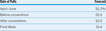
Forecasts made at other points in the election year were strikingly similar to our “official” forecast (see table 2). Our July 1 forecast using the LEI measure and polls from the second quarter of 2016 was 52.2% for Clinton. Footnote 10 A later forecast substituting polls from just before the first convention was 52.0%, exactly as we forecasted after the conventions. Plugging polls for the final week of the campaign (from Real Clear Politics) into our quarter 16 model predicts a little lower 51.4%. Footnote 11 Although our specific predictions changed some over time, broad electoral expectations remained much the same.
Forecasts of the Clinton Vote Share at Different Points in 2016

Note: Based on models including the quarter 13 measure of cumulative growth in leading economic indicators and also trial-heat polls measured at various points of the election timeline. The equations are all based on data from the 16 elections between 1952 and 2012. For the details, see Erikson and Wlezien (Reference Erikson and Wlezien2016).
Even more than usual, the media narrative about 2016 was about the (uniquely unpopular) candidates and their campaigns. Despite frequent predictions by pundits that Trump’s candidacy was doomed, the post-conventions campaign played out very much like our projections based solely on the early economy and early polling. Did the fundamentals win out? In the final analysis, Trump’s strength and weaknesses as a candidate offset those of Clinton, whose candidacy was weighted down by WikiLeaks revelations and the fallout of FBI investigations of her e-mail problem.
THE ECONOMIC PESSIMISM MODEL
The economic pessimism model performed strongly this year. The model forecast the Democratic candidate to get 50.4% of the two-party vote. The final vote count gave the incumbent party 51.1% of the two-party vote, yielding an error of less than a percentage point. This is especially impressive given that the forecast was made 133 days before the election. The model is available well before the election. Moreover, with only two independent variables, the model is parsimonious. Running the equation with the additional data point does not change matters consequentially; the point estimates are virtually identical. The economic item increases by less than .001 and the time in the White House changes by less than .10. The model is very stable.
The campaign featured a reality tv show personality and presumed billionaire who regularly made what were thought to be disqualifying statements from the first day of the campaign through almost the end. Many pundits predicted a landslide victory for the incumbent party through early in the evening of election day. A model looking at the fundamentals of the campaign produced a much more accurate forecast of the outcome well in advance of the election. Political scientists, unlike many others, did a good job of forecasting a close election.
The results of the House model were similarly strong. The model forecast a zero seat change in the House. The actual change is a 6 seat loss. Running the equation with the additional data point does not alter the interpretation at all. The economic item is identical to the earlier result. The open seat interaction item changes by .01. The only item that changes appreciably is the time in the White House variable. Still, in neither case is it significant.
Looking forward to 2020, as it will be a first bid for reelection, the Republicans are in a good position to retain the White House. Even if the economy is perceived as negatively as it was in the spring 0f 2016, they should do quite well. In fact, the incumbent party would be predicted to win with approximately 55% of the two-party vote.
POST-MORTEM: NATIONAL CONDITIONS AND TRIAL-HEAT POLLS
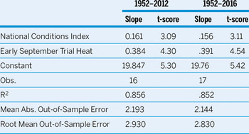
It may sound a bit odd to say that the 2016 election went pretty much according to form, but viewed from the perspective of the popular vote totals, that appears to be the case, at least based on predictions from the National Conditions and Trial-Heat model. The model, which incorporates an index of national conditions measured during the summer prior to the election and trial-heat poll results from the first week in September, predicted that Hillary Clinton would receive 52.5% of the two-party popular vote, whereas she ended up with 51.1% of the two-party vote. The error in this prediction (1.4 points) is somewhat smaller than the average absolute error (2.19 points) from previous out-of-sample estimates from the same model (see table 3). In the updated model, which incorporates the 2016 election result, there are only very slight changes to the slopes and fit statistics, compared the 1952–2012 model, again confirming that the 2016 outcome was very close to what the model projected.
The National Conditions and Trial-Heat Model before and after the 2016 Election

Note: The index of national conditions is comprised of presidential approval (Gallup) and aggregate satisfaction with personal finances (Survey of Consumers), both averaged over June, July, and August of election years. The trial-heat variable is the average of the incumbent party percent of the expressed two-party vote in Gallup trial-heat polls taken in the first week of September (or earliest polls in September if none in the first week) of the election year. In years in which one of the nominating conventions is held in early September, the trial-heat polls are taken from the week after the last day of the convention. In 2016, Gallup did not release presidential trial-heat polls, so the average of all publicly available polls during the first week in September were used.
Of course, the 2016 election did not go according to form in other important ways, and Donald Trump’s Electoral College victory despite a substantial popular vote loss might illustrate the potential folly of forecasting elections based on popular votes. At the very least, the 2016 outcome should serve as a reminder that we are predicting the national popular vote winner, not the winner of the presidential election.
THE STATE-BY-STATE POLITICAL ECONOMY MODEL: BETWEEN SEMI-SUCCESS AND SEMI-FAILURE
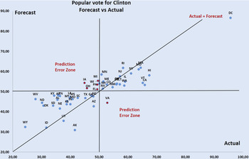
Two and a half months before the 2016 US election our State-by-State Political Economy Model (PEM) gave a slight advantage to Hillary Clinton with 50.15% of the popular vote (error margin +/- 4.6%) and 319 electoral votes (See PS 49 (4): 680–86). In the end, on November 8, 2016 the Democratic candidate actually won the (two-party) popular vote with 51.1%, however she only had 232 electoral votes and Donald Trump has been elected the 45th President of the United States.
Thus, our model successfully predicted the correct Democratic/Republican balance of power with regard to popular vote but this was not enough to ensure a satisfactory result. Indeed, this is the first time of our PEM fails since its first run in 2004.
If we look at the balance between forecasts and achievements, the model did not correctly predict the results in FL, IA, MI, OH, PA, VA, and WI (see figure 1).
State-by-State Political Economy Model Forecast for 2016 Presidential Election

Two key states are clearly in the error margin (FL and PA, e.g. 49 EVs) but this does not absolve us from seeking possible explanations.
If we consider our main variables, Hillary Clinton had no rational reason to lose MI, OH, or WI. First, Obama’s popularity (52.5% in August 2016) was a major plus. Secondly, in these Rust Belt states, we observe a faster decrease in unemployment (over 20-quarters) compared to national level. Moreover, still in MI, OH, and WI, Donald Trump underperformed his national score at GOP primaries (e.g. 44.95%). At last, in each of those cases, our partisan domination index was mostly in favor of the Democratic candidate. In contrast, the decrease in unemployment was far less swift in IA, PA, and VA. Note that Donald Trump overperformed his national score at primaries in FL and PA. Aside from VA, Footnote 12 it seems that IA, PA, and FL had certain weaknesses potentially detrimental to Clinton but the PEM was not sensitive enough to detect them.
All things considered, the treatment of both popularity and partisan domination seem to have been imperfect. If we observe the state level popularity (Gallup), Obama’s job approval is significantly below his national level in IA (-5.5), OH (-4.5), PA (-3,5) and WI (-1.5). However, a small surplus is found in FL (+0.5), MI (+1.5), and VA (+0.5).
Furthermore, our partisan domination index captures long-term effects but not short-term ones. In this regard, the Gallup state-level party identification show that the feeling to be close to Republicans is above the average level (40.1%) in each of our errors except in MI. Likewise, the identification to Democratic party is below the national level (43%) everywhere notwithstanding PA.
A preliminary simulation aiming to include state-level popularity and party identification would allow to forecast correctly IA and PA only (e.g. 26 EVs). Unfortunately, states such as FL, MI, or WI stand unpredictable.
Drawing on this, which direction should be taken to improve our model? For instance, we could add incumbent’s main rival score at primaries. Bernie Sanders overperformed in IA, MI, PA, and WI. This apart, is such a variable accurate for each election since (at least) 1980? Doubts remain about this.
More specifically, we should experiment the insertion of an index synthesizing several local sociodemographic characteristics such as those which likely helped Donald Trump to win, despite the loss of the popular vote.
THE 2016 POLLYVOTE POPULAR VOTE FORECAST: A PRELIMINARY ANALYSIS
Since its launch last January, the 2016 PollyVote consistently predicted that Hillary Clinton would win the popular vote, which she did. In this preliminary analysis we assess how the PollyVote and its components performed in this election compared to the previous six (1992 to 2012).
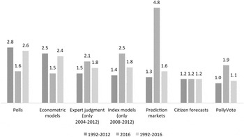
Ranked according to their historical accuracy from best to worst, right to left in figure 2, the six components of the PollyVote place as follows: citizen forecasts, prediction markets, index models, expert judgment, econometric models, and polls. In 2016 citizen forecasts Footnote 13 defended their top position, but other methods were outliers relative to their historical record. Both polls and econometric models performed considerably better, while prediction markets did worse. This fluctuation in accuracy among methods makes it difficult to predict ex ante which method will do best.
Forecast Error by PollyVote Component Method: Mean absolute error, historical vs. 2016, across last 100 days before the election

Combining forecasts within and across methods, as the PollyVote does, guarantees that its forecast will never come out last and will always do at least as well as the typical forecast. Footnote 14 This was demonstrated this year. The PollyVote incurred an error of 1.9 percentage points, almost twice the historical average, but lower than that of three other methods.
Combining works best when the various component forecasts bracket the true value (Graefe et al., Reference Graefe, Armstrong, Jones and Cuzán2014a). Compared to the previous six elections, there wasn’t much bracketing in 2016. Five of the combined forecasts overshot Clinton’s share of the vote while only one component, the econometric models, fell short. Thus the PollyVote did not do as well as in previous elections.
The method of combining forecasts makes no claim that the PollyVote will always outperform its most accurate component, although that can happen, as was the case in 2004 (Cuzán et al., Reference Cuzán, Armstrong and Jones2005) and 2012 (Graefe et al. Reference Graefe, Armstrong, Cuzán and Jones2014b). What is claimed is that over time, as the constituent methods’ relative accuracy varies, the PollyVote will surpass them. This is demonstrated in figure 2, which displays the mean absolute error of all methods across all seven elections from 1992 to 2016. On average, then, the PollyVote continues to minimize error while avoiding making large errors.